Blind multiclass ensemble classification

Blind Multiclass Ensemble Classification

Panagiotis A. Traganitis,

Student Member, IEEE,

Alba Pag`es-Zamora,

Senior Member, IEEE,

and Georgios B. Giannakis,

Fellow, IEEE

Abstract—The rising interest in pattern recognition and data analytics has spurred the development of innovative machine learning algorithms and tools. However, as each algorithm has its strengths and limitations, one is motivated to judiciously fuse multiple algorithms in order to find the “best” performing one, for a given dataset. Ensemble learning aims at such high-performance meta-algorithm, by combining the outputs from multiple algorithms. The present work introduces a blind scheme for learning from ensembles of classifiers, using a moment match-ing method that leverages joint tensor and matrix factorization. Blind refers to the combiner who has no knowledge of the ground-truth labels that each classifier has been trained on. A rigorous performance analysis is derived and the proposed scheme is evaluated on synthetic and real datasets.

Index Terms—Ensemble learning, unsupervised, multiclass classification, crowdsourcing.

I. INTRODUCTION

T

HE massive amounts of generated and communicated data has introduced society and computing to a data “deluge.” Along with the increase in the amount of data, multiple machine learning, signal processing and data mining algorithms have been developed. These algorithms are usually tailored for different datasets, and they often operate under dif-ferent assumptions. As such, finding an algorithm that works “well” for a specific dataset can be prohibitively complex or impossible.

Ensemble learning refers to the task of designing a meta-learner, by combining the results provided by multiple dif-ferent learners or annotators1; see Fig. 1. This meta-learner should generally be able to outperform the individual learners. In particular, ensemble classification refers to fusing the results provided by different classifiers. Each classifier observes data, decides one class, out ofKpossible, each of these data belong to, and provides the meta-learner with those decisions. Such a setup emerges in diverse disciplines including medicine [1], biology [2], team decision making and economics [3], and has recently gained attention with the advent of crowdsourcing [4], as well as services such as Amazon’s Mechanical Turk [5], CrowdFlower and Clickworker, to name a few. A related setup appears in distributed detection [6], [7], where sensors collect data, decide which one out of K possible hypotheses is in Panagiotis A. Traganitis and Georgios B. Giannakis are with the Dept. of Electrical and Computer Engineering and the Digital Technology Center, University of Minnesota, Minneapolis, MN 55455, USA.

Alba Pag`es-Zamora is with the SPCOM Group, Universitat Polit`ecnica de Catalunya BarcelonaTech, Spain.

Work supported by NSF grants 1500713 and 1514056, as well as by “Ministerio de Econom´ıa y Competitividad” of the Spanish Government, ERDF funds (TEC2015-69648-REDC,TEC2016-75067-C4-2-R).

Emails:{[email protected], [email protected], [email protected]}

1_{The terms learner, annotator, and classifier will be used interchangeably}

throughout this manuscript.

effect, and transmit those decisions to a fusion center, that makes a final decision. A similar task is also known as the CEO problemor multiterminal source coding [8].

When training data are available, a meta-learner can learn how to combine the results from individual classifiers, based on these ground-truth labels [9]. One such approach is boost-ing [10], where multiple classifiers are combined accordboost-ing to their probability of error on the training set. In the boosting regime, each classifier is also using information from the rest. In many cases however, labeled data are not available to train the combining meta-classifier, and/or, the individual classifiers cannot be retrained, justifying the need for unsupervised (or blind) ensemble learning methods. One such paradigm is provided by crowdsourcing, where people are tasked with providing classification labels. Accordingly, in a distributed detection setup, the fusion center might not have access to the sensors, once they have been deployed.

The present work puts forth a novel scheme formulticlass blind ensemble classification, built upon simple concepts from probability and detection theory, as well as recent advances in tensor decompositions [11] and optimization theory, that enable assessing the reliability of multiple annotators and combining their answers. Under our proposed model, each annotator has a fixed probability of deciding that a datum belongs to class k, given that the true class of the datum is k0. Assuming that annotators make decisions independent of each other, the proposed method extracts these probabilities from the first-, second-, and third-order statistics of annotator responses. This becomes possible thanks to a joint PARAFAC decomposition, which has been employed in a related problem of identifying conditional probabilities to complete a joint probability functions from its projections [12]. The crux of our algorithm is a moment matching method, that leverages the aforementioned PARAFAC decomposition approach to obtain accurate estimates of annotator decision probabilities along with class priors. These estimates are then provided to the meta-detector to form the final estimate of data labels.

To assess the proposed scheme, extensive numerical tests, on synthetic as well as real data are presented, comparing the proposed approach to state-of-the-art binary and multiclass blind ensemble classification methods. In addition, a rigorous performance analysis is provided, which showcases the con-ditions under which our novel method works.

The rest of the paper is organized as follows. Section II states the problem, provides preliminaries for the proposed approach along with a brief description of the prior art in unsupervised ensemble classification. Section III introduces the proposed scheme for multiclass unsupervised ensemble classification, while Section IV analyses the performance of the proposed method. Section V presents numerical tests to

Data x

Learner 1 Learner 2 . . . LearnerM

Meta-learner/Fusion center ˆ

y

f1(x) f2(x) fM(x)

Fig. 1. Unsupervised ensemble classification setup, where the outputs of learners are combined in parallel.

compare our method with state-of-the-art ensemble classi-fication algorithms. Finally, concluding remarks and future research directions are given in Section VI. Detailed deriva-tions are delegated to Appendix A, while proofs of theorems, propositions and lemmata are deferred to Appendix B.

Notation: Unless otherwise noted, lowercase bold letters,x,

denote vectors, uppercase bold letters,X, represent matrices, and calligraphic uppercase letters, X, stand for sets. The (i, j)th entry of matrix X is denoted by [X]ij; and its rank

by rank(X); X> denotes the tranpose of matrix X; RD

stands for the D-dimensional real Euclidean space, R+ for the set of positive real numbers, Z+ for the set of positive integers, E[·] for expectation, and k · k for the `2-norm. Underlined capital lettersXdenote tensors, vec(·)denotes the vectorization operator, that stacks columns of a matrix into a longer column vector; the vector outer product is denoted by ◦, and, denotes the Khatri-Rao matrix product. For a 3-mode tensor X, X(:,:, i),X(:, i,:), and X(i,:,:) denote the i-th frontal, longitudinal and lateral slabs of X, respectively, while X(i, j, l)denotes theijl-th element ofX.

II. PROBLEMSTATEMENT ANDPRELIMINARIES Consider a dataset consisting of N data (possibly vectors) {xn}Nn=1 each belonging to one of K possible classes with corresponding labels {yn}Nn=1, e.g. yn =k if xn belongs to

class k. The pairs {(xn, yn)} are drawn independently from

an unknown joint distributionD, andXandY denote random variables such that (X, Y)∼D. Consider nowM annotators that observe {xn}Nn=1, and provide estimates of labels. Let fm(xn) ∈ {1, . . . , K} denote the label assigned to datum xn by the m-th annotator. All annotator responses are then

collected at a centralized meta-learner or fusion center. The task ofunsupervised ensemble classificationis: Given only the annotator responses{fm(xn), m= 1, . . . , M}Nn=1, we wish to estimate the ground-truth labels of the data {yn}; see Fig. 1.

Similar to unsupervised ensemble classification, crowd-sourced classification seeks to estimate ground-truth labels of the data {yn} from annotator responses {fm(xn)}, with the

additional caveat that each annotatormmay choose to provide labels for only a subsetNm< N of data.

A. Prior work

Probably the simplest scheme for blind or unsupervised ensemble classification is majority voting, where the estimated

label of a datum is the one that most annotators agree upon. Majority voting has been used in popular ensemble schemes such as bagging, and random forests [13]. While relatively easy to implement, majority voting presumes that all annotators are equally “reliable,” which is rather unrealis-tic, both in crowdsourcing as well as in ensemble learning setups. Other blind ensemble methods aim to estimate the parameters that characterize the annotators’ performance. A joint maximum likelihood (ML) estimator of the unknown labels and these parameters has been reported using the expectation-maximization (EM) algorithm [14]. As the EM algorithm does not guarantee convergence to the ML solution, recent works pursue alternative estimation methods. For binary classification, [15] assumes that annotators adhere to the “one-coin” model, meaning each annotator m provides the correct (incorrect) label with probability δm (1−δm); see

also [16] when annotators do not label all the data, and [17] for an iterative method. Recently, [18], [19] advocated a spectral decomposition technique of the second-order statistics of annotator responses for binary classification, that yields the reliability parameters of annotators, when class probabilities are unknown, while [20] introduced a minimax optimal algo-rithm that can infer annotator reliabilities. In the multiclass setting, [17] solves multiple binary classification problems. In addition, [21] and [22] utilize third-order moments and orthog-onal tensor decomposition to estimate the unknown reliability parameters and then initialize the EM algorithm of [14]. This procedure however, can be numerically unstable, especially when the number of classes K is large, and classes are unequally populated. Finally, all the methods mentioned in this section employ ML estimation, which implicitly assumes that the dataset is balanced, meaning classes are roughly equiproba-ble. Another interesting approach is presented in [23], where a joint moment matching and maximum likelihood optimization problem is solved.

The present work puts forth a novel scheme formulticlass blind ensemble classification, built upon simple concepts from probability and detection theory. It relies on a joint PARAFAC decomposition approach, which lends itself to a numerically stable algorithm. At the same time, our novel approach takes into account class prior probabilities to yield accurate esti-mates of class labels. Compared to our conference precursor in [24], here we do not require the prior probabilities to be known, and we present comprehensive numerical tests, along with a rigorous performance analysis.

B. Canonical Polyadic Decomposition/PARAFAC

This subsection will outline tensor decompositions, which will be used in the following sections to derive the proposed scheme. Consider a 3-modeI×J×L tensorX, which can be described by a matrix in 3 different ways

X(1) := [vec(X(1,:,:)), . . . ,vec(X(I,:,:))] (1a)

X(2):= [vec(X(:,1,:)), . . . ,vec(X(:, J,:))] (1b)

where X(1) _{is of dimension J L×I, X}(2) _{is IL×J and}

X(3) _{is IJ ×L. Under the Canonical Polyadic} Decomposi-tion(CPD)/Parallel Factor Analysis (PARAFAC) model [25], X can be written as a sum of R rank one tensors (a.k.a. factors) X = R X r=1 ar◦br◦cr (2)

where ar,br,cr are I×1, J×1 and L×1 vectors,

respec-tively. Letting A := [a1, . . . ,aR],B := [b1, . . . ,bR], and

C:= [c1, . . . ,cR]be the so-called factor matrices of the CPD

model, we write (2) compactly as

X = [[A,B,C]]R (3)

and (1) can be equivalently written as

X(1)= (CB)A> (4a)

X(2)= (CA)B> (4b)

X(3)= (BA)C> (4c) where we have used the fact that for matrices A,B

and a vector c of appropriate dimensions, it holds that vec(Adiag(c)B>) = (BA)c. By vectorizing X(3), it is easy to show that the vectorization of the entire tensor will be of the form x := vec(X) = vec(X(3)_{) = (CBA)1.} Accordingly, vectorizing X(1) _{or X}(2) _{produces different} vectorizations of the entire tensor, where the order of factor matrices in the Khatri-Rao product is permuted. Recovery of the factor matrices A,B andC, can be done by solving the following non-convex optimization problem

[ ˆA,Bˆ,Cˆ] = arg min A,B,C

kX−[[A,B,C]]Rk2F. (5)

Similar to the matrix case, the Frobenius norm here can be defined as kXkF :=

q_P

i,j,lX(i, j, l)2, and as (4) is just a

rearrangement of the terms inX, it holds that

kXkF =kX(1)kF =kX(2)kF =kX(3)kF. (6)

Typically, (5) is solved using alternating optimization (AO) or gradient descent [11]. Multiple off-the-shelf solvers are avail-able for PARAFAC tensor decomposition; see e.g. [26], [27]. Furthermore, depending on extra properties of X, constraints can be enforced on the factor matrices, such as nonnegativity and sparsity to name a few, which can be effectively handled by popular solvers such as AO-ADMM [28]. Under certain conditions, the factorization of X into A,B, and C, is essentially unique, oressentially identifiable, that isAˆ,Bˆ, and

ˆ

C can be expressed as ˆ

A=APΛa, Bˆ =BPΛb, Cˆ =CPΛc (7)

where P is a common permutation matrix, and Λa,Λb,Λc

are diagonal scaling matrices such that ΛaΛbΛc = I [11].

For more details regarding the PARAFAC decomposition and tensors with more than3modes, interested readers are referred to the comprehensive tutorial in [11] and references therein.

III. UNSUPERVISEDENSEMBLECLASSIFICATION Each annotator in our model has a fixed probability of deciding that a datum belongs to class k0, when presented with a datum of class k. Thus, each annotator m can be characterized by a so called confusion matrix Γm, whose

(k0_{, k)-th entry is}

[Γm]k0_k:= Γ_m(k0, k) = Pr (f_m(X) =k0|Y =k). (8)

TheK×KmatrixΓmhas non-negative entries that obey the

simplex constraint, since PK

k0₌₁Pr (fm(X) =k0|Y =k) =

1, for k= 1, . . . , K; hence, entries of eachΓm column sum

up to1, that is,Γ>_m1=1andΓm≥0. The confusion matrix

showcases the statistical behavior of an annotator, as each column provides the annotator’s probability of deciding the correct class, when presented with a datum from each class. Before proceeding, we adopt the following assumptions.

As1. Responses of different annotators per datum, are condi-tionally independent, given the ground-truth label Y of the same datumX; that is,

Pr (f1(X) =k1, . . . , fM(X) =kM|Y =k) = M Y m=1 Pr (fm(X) =km|Y =k)

As2. Most annotators are better than random; e.g., most have probability of correct detection exceeding0.5forK= 2. Clearly, for annotators that are better than random, the largest elements of each column of their confusion matrix will be those on the diagonal ofΓm; that is

[Γm]kk≥[Γm]k0_k, for k0, k= 1, . . . , K.

As1 suggests that annotators make decisions independently of each other, which is rather a standard assumption [14], [19], [22]. Likewise, As2 is another standard assumption, used to alleviate the inherent permutation ambiguity of the confusion matrix estimates provided by our algorithm. Note that As2 is slightly more relaxed than the corresponding assumption in [22], which splits annotators into 3 groups and requires most annotators in each group to be better than random.

A. Maximum a posteriori label estimation

Given only annotator responses for all data, a straight-forward approach to estimating their ground-truth labels is through a maximum a posteriori (MAP) classifier [29]. In particular, for datumX the MAP classifier is

ˆ

yMAP(X) = arg max

k∈{1,...,K}L(X|k) Pr(Y =k) (9)

whereL(X|k) := Pr (f1(X) =k1, . . . , fM(X) =kM|Y =k)

is the conditional likelihood of X. As annotators make independent decisions, it holds that L(X|k) =

QM

m=1Pr (fm(X) =km|Y =k), and thus the MAP classifier

can be rewritten as ˆ

yMAP(X) = arg max k∈{1,...,K} logπk+ M X m=1 log(Γm(km, k)) (10)

where πk := Pr(Y = k). It is well known from detection

theory [29] that the MAP classifier (10) minimizes the average probability of errorPe, given by

Pe = K X

k=1

πkPr(ˆyMAP=k06=k|Y =k). (11) If all classes are equiprobable, that is πk = 1/K for all k= 1, . . . , K, then (10) reduces to the ML classifier. In order to obtain the MAP or ML classifier, {Γm}Mm=1must be avail-able, while in the MAP classifier case π:= [π1, . . . , πK]> is

also required. Interestingly, the next section will illustrate that {Γm}Mm=1andπshow up in (and can thus be estimated from) the moments of annotator responses.

B. Statistics of annotator responses

Consider each label represented by the annotators using the canonical K ×1 vector ek, denoting the k-th column

of the K ×K identity matrix I. Let fm(X) denote the m-th annotator’s response in vector format. Since fm(X)

is just a vector representation of fm(X), it holds that

Pr (fm(X) =k0|Y =k) ≡ Pr (fm(X) =ek0|Y =k). With

γm,k denoting thek-th column of Γm, it thus holds that

E[fm(X)|Y =k] = K X k0₌₁ ek0Pr (f_m(X) =k0|Y =k) (12) =γm,k

where the first equality comes from the definition of con-ditional expectation, and the second one because ek’s are

columns of I. Using (12) and the law of total probability, the mean vector of responses from annotatorm, is hence

E[fm(X)] = K X

k=1

E[fm(X)|Y =k] Pr (Y =k) =Γmπ. (13)

Upon defining the diagonal matrixΠ:=diag(π), theK×K cross-correlation matrix between the responses of annotators m andm06=m, can be expressed as

Rmm0 :=_E[f_m(X)f_m>0(X)] = K X k=1 E[fm(X)|Y =k]E[fm>0(X)|Y =k] Pr (Y =k) =Γmdiag(π)Γ>m0 =ΓmΠΓ>m0 (14)

where we successively relied on the law of total probability, As1, and (12). Consider now theK×K×Kcross-correlation tensor between the responses of annotators m,m0 6=m and m006=m0, m, namely

Ψ_mm0_m00=_E[fm(X)◦fm0(X)◦f_m00(X)]. (15)

It can be shown thatΨ_mm0_m00 obeys a CPD/PARAFAC model

[cf. Sec. II-B] with factor matricesΓm,Γm0 andΓ_m00; that is,

Ψmm0_m00= K X k=1 πkγm,k◦γm0_,k◦γ_m00_,k (16) = [[ΓmΠ,Γm0,Γ_m00]]_K.

Note here that the diagonal matrixΠ can multiply any of the factor matricesΓm,Γm0, or,Γ_m00.

With Fm := [fm(x1),fm(x2), . . . ,fm(xN)] the sample

mean of them-th annotator responses can be readily obtained as µm= 1 N N X n=1 fm(xn) = 1 NFm1. (17)

Accordingly, the K×K sample cross-correlation Smm0

ma-trices between the responses of annotators m andm0 6= m, are given by Smm0 = 1 N N X n=1 fm(xn)fm>0(xn) = 1 NFmF > m0. (18)

Lastly, the sample K × K ×K cross-correlation tensors T_mm0_m00 between the responses of annotators m, m0 6= m

andm006=m, m0 are T_mm0_m00= 1 N N X n=1 fm(xn)◦fm0(x_n)◦f_m00(x_n) (19) = 1 NFm◦Fm0◦Fm00. Clearly, Smm0 =S>_m0_m, T (2) m0_mm00 =T (3) m0_m00_m = T (1) mm0_m00.

In addition, asN increases, the law of large numbers (LLN) implies that,{µm},{Smm0}, and{T_mm0_m00} approach their

ensemble counterparts in (13), (14), and (15).

Having available first-, second-, and third-order statistics of annotator responses, namely {µm}Mm=1, {Smm0}M_m,m0₌₁,

and {T_mm0_m00}M

m,m0_,m00₌₁, estimates of {Γm}Mm=1 and π can be readily extracted from them [cf. (13), (14), (15)]. This procedure corresponds to the method-of-moments estima-tion [30]. Upon obtaining{Γˆm}Mm=1andπˆ, the MAP classifier of Sec. III-A can be subsequently employed to estimate the label for each datum. That is, forn= 1, . . . , N,

ˆ

yMAP(xn) = arg max k∈{1,...,K} log ˆπk+ M X m=1 log ˆΓm(fm(xn), k) (20) where Γˆm(k0, k) = [ ˆΓm]k0_k, and ˆπ_k = [ ˆπ]_k. The following

section provides an algorithm to estimate these unknown quantities.

C. Confusion matrix and prior probability estimation To estimate the unknown confusion matrices and prior probabilities consider the following non-convex constrained optimization problem, min π {Γm}M m=1 hN({Γm}Mm=1,π) (21) s.to Γm≥0, Γ>m1=1, m= 1, . . . , M π≥0, π>1= 1

Algorithm 1 Confusion matrix and prior probability estima-tion algorithm

Input: Annotator responses {Fm}Mm=1, λ > 0, ν > 0;

maximum number of iterationsI∈_Z+

Output: Estimates of{Γˆm}Mm=1 andπˆ

1: Compute {µm},{Smm0},{T_mm0_m00} using (17),

(18), and (19).

2: Initialize{Γm} andπ randomly. 3: do 4: form= 1, . . . , M do 5: UpdateΓm using (23) 6: Γ(prev)m ←Γm 7: end for 8: Updateπ using (22) 9: π(prev)_←π 10: i←i+ 1

11: whilenot converged and i < IT

12: Find permutation matrix Pˆ, such that the majority of {ΓˆmPˆ}Mm=1 satisfy As2.

Algorithm 2 Unsupervised multiclass ensemble classification

Input: Annotator responses{Fm}Mm=1

Output: Estimates of data labels {yˆn}Nn=1

1: Find estimates{Γˆm}Mm=1 andπˆ using Alg. 1 2: forn= 1, . . . , N do

3: Estimate labelyn using (20).

4: end for where hN({Γm},π) := 1 2 M X m=1 kµm−Γmπk22 +1 2 M X m=1 m0>m kSmm0−Γ_mΠΓ>_m0k2_F +1 2 M X m=1 m0>m m00>m0 kT_mm0_m00−[[ΓmΠ,Γm0,Γ_m00]]_Kk2_F

and the subscript N inhN denotes the number of data used

to obtain annotator statistics. Collect the set of constraints per matrix to the convex set C :={Γ∈_RK×K _{: Γ≥0,Γ}>₁₌ 1}, where essentially each column lies on a probability sim-plex, and let Cp:={u∈RK :u≥0,u>1= 1} denote the

constraint set for π.

As (21) is a non-convex problem, alternating optimization will be employed to solve it. Specifically the alternating optimization-alternating direction method of multipliers (AO-ADMM) will be employed; see [28], and also [12] where a similar formulation appears. Under the AO-ADMM paradigm, hN is minimized per block of unknown variables{Γm} orπ

while the other blocks remain fixed, as in block coordinate descent schemes. Solving for one block of variables with the remaining fixed is a convex constrained optimization problem under convex C and Cp constraint sets. These optimization

problems are pretty standard and several solvers are available,

including proximal splitting methods, projected gradient de-scent or ADMM [31]–[34]. Here, the solver of choice for each block of variables will be ADMM.

The update forπ involves minimizinghN with{Γm}Mm=1 fixed. Specifically, the following problem is solved

min π∈Cp gN,π(π) (22) where gN,π(π) := 1 2 M X m=1 kµm−Γmπk22+ ν 2kπ−π (prev)_k2 2 +1 2 M X m=1 m0>m ksmm0−(Γ_m0Γ_m)πk2₂ +1 2 M X m=1 m0>m m00>m0 ktmm0_m00−(Γ_m00Γ_m0Γ_m)πk2₂ smm0 = vec(S_mm0), t_mm0_m00 = vec(T(3)_mm0_m00)

[cf. (4)], ν is a positive scalar, and we have used vec(Γmdiag(π)Γ>m0) = (Γm0Γ_m)π and

vec([[Γmdiag(π),Γm0,Γ_m00]]_K) = (Γ_m00 Γ_m0 Γ_m)π.

Note that gN,π contains all of the terms in hN along with

(ν/2)kπ−π(prev)k2

2, which is included to ensure convergence of the AO-ADMM iterations to a stationary point of (21) [28], [35]. Here,π(prev) _{denotes the estimate ofπ obtained by the} previous solutions of (22).

Accordingly per Γm, the following subproblem is solved

with{Γm0}M m0_6=m andπ fixed min Γm∈C gN,m(Γm) (23) where gN,m(Γm) := 1 2kµm−Γmπk 2 2+ ν 2kΓm−Γ (prev) m k 2 F +1 2 M X m0_6=m kSm0_m−Γ_m0ΠΓ>_mk2_F +1 2 M X m0_>m m00>m0 kT(1)_mm0_m00−(Γm00Γ_m0)ΠΓ>_mk2_F T(1)_mm0_m00 = [vec(T(1,:,:)), . . . ,vec(T(K,:,:))], Γ (prev) m

de-notes the estimate of Γm obtained by the previous solution

of (23), ν is a positive scalar, and we have used (6). Here, gN,m contains all the terms of hN that involve Γm with

the additional term (ν/2)kΓm−Γ (prev)

m k2F, which ensures

convergence of the AO-ADMM iterations.

Detailed derivations of the ADMM iterations for solving (23) and (22) are provided in Appendix A, while the AO-ADMM is summarized in Alg. 1. The computational com-plexity of the entire AO-ADMM scheme is approximately O(ITM3K4), where IT is the number of required iterations

until convergence (see Appendix A-C). The entire unsuper-vised ensemble classification procedure is listed in Alg. 2.

D. Convergence and identifiability

Convergence of the entire AO-ADMM scheme for (21), follows readily from results in [28, Prop. 1], stated next for our setup.

Proposition 1. [28, Prop. 1]Alg. 1 for M ≥3, andν > 0

converges to a stationary point of (21).

Having established the convergence of Alg. 1 to a stationary point of (21) using Prop. 1, the suitability of the estimates provided by Alg. 1 for the ensemble classification task needs to be assessed. As (21) involves joint tensor decompositions, under certain conditions the solutions {Γˆm},πˆ of (21) will

be, similar to the PARAFAC decomposition of Sec. II-B, essentially unique. Thus, in order to assess the suitability of the estimates provided by Alg. 1 the conditions under which the model employed in (21) is identifiable have to be established. Luckily, identifiability claims for the present problem can be easily derived from recent results in joint PARAFAC factorization [12], [36].

Lemma 1. Let {Γ∗_m}, π∗ be the optimal solutions of (21),

and{Γˆm},πˆ the estimates provided by Alg. 1. If at least three {Γm}Mm=1 have full column rank, there exists a permutation matrix Pˆ such that

ˆ

ΓmPˆ =Γ∗m, m= 1, . . . , M, Pˆ

>_πˆ=π∗_.

Lemma 1 essentially requires that at least three annotators respond differently to different classes, that is no two columns of at least three confusion matrices are colinear. Possibly more relaxed identifiability conditions could be derived using techniques mentioned in [36]. Unlike the tensor decomposition mentioned in Sec. II-B, here we have no scaling ambiguity on the confusion matrices or prior probabilities. This is important because there are infinite scalings, but finite permutation matrices sinceKis finite. Under As2,Pˆ can be easily obtained since the largest elements of each column of a confusion matrix must lie on the diagonal for the majority of annotators. EachΓˆmcan be multiplied by a permutation matrixPˆm, such

that the largest elements are located on the diagonal. The final ˆ

Pcan be derived as the most commonly occurring permutation matrix out of {Pˆm}Mm=1.

Remark 1. While we relied on statistics of annotator

re-sponses up to order three, higher-order statistics can also be employed. Higher-order moments however, will increase the complexity of the algorithm, as well as the number of data required to obtain reliable (low-variance) estimates.

Remark 2. Estimates of annotator confusion matrices{Γˆm}

and data labels {yˆn}, provided by Alg. 2, can be used to

initialize the EM algorithm of [14].

Remark 3. The orthogonal tensor decomposition used by

[21], [22] is a special case of the PARAFAC decomposition employed in this work.

Remark 4. When π is known, (22) can be skipped, and

correspondingly steps 8 and9 of Alg. 1.

E. Reducing complexity

When K and M are large Alg. 1 may require long computational time to converge. Our idea in this case is to split the annotators into L groups, and solve (21) for each group. For simplicity of exposition, consider non-overlapping groups, each with M` ≥ 3 annotators (P

L `=1M` = M). Letµ(m`),S (`) mm0 andT (`)

mm0_m00 denote the sample statistics for

annotators in group`, and{Γ(m`)}Mm=1` the confusion matrices in group`.

For each group ` ∈ {1, . . . , L} confusion matrices {Γˆ(m`)}Mm=1` and prior probabilitiesπ

(`)_{are estimated by} solv-ing a smaller version of (21), namely

min π(`) {Γ(m`)}M m=1 h(_N`)({Γ(<sub>m</sub>`)}M m=1,π (`)<sub>)</sub> (24) s.to Γ(<sub>m</sub>`)≥0, 1>Γ_m(`)=1>, m= 1, . . . , M` π(`)≥0, 1>π(`)= 1 where h(_N`)({Γm},π) := 1 2 M` X m=1 kµ(_m`)−Γmπk22 +1 2 M` X m=1 m0>m kS(_mm`) 0−ΓmΠΓ>m0k2<sub>F</sub> +1 2 M X m=1 m0>m m00>m0 kT(<sub>mm</sub>`) 0_m00−[[ΓmΠ,Γm0,Γ_m00]]_Kk2_F.

Upon solving (24) for allLgroups, estimates of{Γm}Mm=1 are readily obtained, since we have assumed non-overlapping groups. A final estimate of the prior probabilities π can be obtained by averaging theLestimates{π`_}L

`=1. As (24) incurs a complexity ofO(IM3

`K3), the worst-case

complexity of this approach is O(IMK3PL<sub>`=1</sub>M`3), where IM is the largest number of iterations required to converge

among all L groups. SinceM3_{= (}PL

`=1M`)3>P L `=1M`3

this approach reduces the computational and memory overhead significantly compared to Alg. 1. Note however, that this method is expected to perform well when As1 and As2, as well as the conditions outlined in Lemma 1 are satisfied for all L groups of annotators, and N is sufficiently large. The effectiveness of this complexity reduction scheme is tested in Sec. V.

F. Application to crowdsourcing

While crowdsourced classification is a task related to ensem-ble classification, it presents additional challenges. So far it has been implicitly assumed that all annotators provide labels for all{xn}Nn=1. In the crowdsourcing setup however, an annotator mcould provide labels just for a subset ofNm< N data.

Next, we outline a computationally attractive approach, that takes into account only the available annotator responses. If an annotatorm does not provide a label for a datum, his/her response is fm(x) = 0 or fm(x) = 0in vector format. Let Jm(xn)be an indicator function that takes the value 1 when

annotator mprovides a label for xn, and 0 when fm(xn) =

0. To account for such cases, the annotator sample statistics become µm= 1 PN n=1Jm(xn) N X n=1 Jm(xn)fm(xn) (25a) Smm0 = PN n=1Jm(xn)Jm0(xn)fm(xn)f > m0(xn) PN n=1Jm(xn)Jm0(x_n) (25b) T_mm0_m00 (25c) = P nJm(xn)Jm0(x_n)J_m00(x_n)f_m(x_n)◦f_m0(x_n)◦f_m00(x_n) PN n=1Jm(xn)Jm0(x_n)J_m00(x_n) . Upon computing the modified sample statistics of (25), we can obtain estimates of the confusion matrices and prior probabilities in the crowdsourcing setup, via Alg. 1. Finally, the MAP classifier in (20) has to be modified as follows

ˆ

yMAP(x) = arg max k∈{1,...,K} log ˆπk+ M X m=1 Jm(x) log ˆΓm(fm(x), k) (26) to take into account only the available annotator responses for each x.

Having completed the algorithmic aspects of our approach, we proceed with performance analysis.

IV. PERFORMANCEANALYSIS

In this section, performance of the proposed method will be quantified analytically. First, the consistency of the estimates provided by Alg. 1 as N → ∞will be established, followed by a performance analysis for the MAP classifier of Sec. III-A. A. Consistency of Alg. 1 estimates

As N → ∞, the sample statistics in (17), (18), and (19) approach their ensemble counterparts, and we end up with the following optimization problem for extracting annotator confusion matrices and prior probabilities

min

π {Γm}M_m=1

h∞({Γm}Mm=1,π) (27)

s.to Γm∈ C, m= 1, . . . , M, π∈ Cp.

Clearly, the optimal solutions to (27) are the true confusion matrices and prior probabilities. AsNincreases, it is desirable to show that the solutions obtained from Alg. 1 converge to the true confusion matrices and prior probabilities. To this end, techniques from statistical learning theory and stochastic optimization will be employed [37], [38]. Specifically, we will establish the uniform convergence of hN toh∞, which

implies the consistency of the solutions. Define the distance between two sets A,B ⊆Rq, for some q >0, asD(A,B) =

sup_x∈A{infy∈Bkx−yk2}.The following theorem shows that as N increases, the solutions of (21) approach those of (27).

Theorem 1. If S∗ and SN denote the sets of solutions of

problems(27)and(21), respectively, thenD(SN,S∗)→0, as

N → ∞ almost surely.

Under As2 and the conditions outlined in Lemma 1, Alg. 1 can recover the true solutions of (21) or (27). Then, by Thm. 1 we know that asN → ∞the solutions of (21) converge to the solutions of (27), which together with the result of Lemma 1 implies the statistical consistency of the solutions of Alg. 1. As a result, the estimates{Γˆm}Mm=1, andπˆ from Alg. 1 will converge to their true values w.p.1 asN → ∞.

B. MAP classifier performance

With consistency of the confusion matrix and prior prob-ability estimates established, the performance of the final component of the proposed algorithm has to be studied. The behavior of the MAP classifier of Sec. III-A can be quantified in terms of its average probability of error

Pe= K X

k=1

Pr(ˆyMAP=k06=k|Y =k) Pr(Y =k)

Here, a well-known asymptotic result for distributed binary detection under the MAP detector [6] is extended to the multiclass case.

Theorem 2. Under As1, and given {Γm}Mm=1 and π, there

exist constants α >0, β >0 such that the MAP classifier of Sec. III-A satisfies

Pe≤αe−βM.

In words, Theorem 2 suggests that when accurate estimates of {Γm}Mm=1 andπ are available, the error rate decreases at an exponential rate with the number of annotatorsM.

In order to validate our theoretical results and evaluate the performance of the proposed scheme, the following section presents numerical tests with synthetic and real data.

V. NUMERICALTESTS

For K ≥ 2, Alg. 2, using both MAP and ML criteria in step 3, (denoted asAlg. 2 MAPandAlg. 2 MLrespectively) is compared to majority voting, the algorithm of [17] (denoted asKOS), and the EM algorithm initialized both with majority voting and with the spectral method of [22] (denoted as EM + MV andEM + Spectral, respectively). ForK = 2, Alg. 2 is also compared to the binary ensemble learning methods of [19], [20] and [16], denoted as SML, TE and EigenRatio, respectively. For synthetic data, the performance of “oracle” estimators, that is MAP/ML classifiers with true confusion matrices of the annotators, and the true class priors, is also evaluated for benchmarking purposes. The metric utilized in all experiments is the classification error rate (ER), defined as the percentage of misclassified data,

ER=# of misclassified data

N ×100%,

where ER = 100% indicates that all N data have been misclassified, and ER = 0% indicates perfect classification

accuracy. For synthetic data, the average confusion matrix and prior probability estimation error is also evaluated

¯ εCM := 1 M M X m=1 kΓm−Γˆmk1 kΓmk1 = 1 M M X m=1 kΓm−Γˆmk1 ¯ επ:=kπ−πˆk1.

All results represent averages over 10 independent Monte Carlo runs, using MATLAB [39]. In all experiments, the parametersλandνof Alg. 1 are set as suggested in [28], [35]. Vertical lines in some figures indicate standard deviation. For some experiments, classification times (in seconds) required by the ensemble algorithms are also reported. Note that classification times for majority voting and oracle estimators are not reported as the time required by these methods is negligible compared to the rest of the algorithms.

A. Synthetic data

For the synthetic data tests,N ground-truth labels{yn}Nn=1, each corresponding to one out of K possible classes, were generated i.i.d. at random according to π, that is yn ∼ π,

for n = 1, . . . , N. Afterwards, {Γm}Mm=1 were generated at random, such that Γm ∈ C, for all m = 1, . . . , M,

and annotators are better than random, as per As2. Then annotators’ responses were generated as follows: if yn =k,

then the response of annotator mwill be generated randomly according to the k-th column of its confusion matrix, γm,k

[cf. Sec. II], that isfm(xn)∼γm,k.

Tab. I lists the classification ER of different algorithms, for a synthetic dataset withK= 2classes with prior probabilities

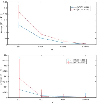
π = [0.9003,0.0997]>, andM = 10 annotators. Tab. II lists the results for a similar experiment, with K = 2 classes, priors π = [0.5856,0.4144]>, and M = 10 annotators, while Tab. III shows the clustering time required by all algorithms. Note that when the class probabilities are similar, the ML and MAP classifiers perform comparably as expected. Furthermore, majority voting gives good results for a reduced number of instances N. Fig. 2 depicts the average estimation errors for the confusion matrices and prior probabilities in the two aforementioned experiments. Clearly, as N increases, the proposed classifiers approach the performance of the oracle ones, and as suggested by Thm. 1, the estimation error for the confusion matrices and prior probabilities approaches 0.

The next synthetic data experiment investigates how the proposed method performs when presented with multiclass data. Furthermore, to showcase that accurate estimation of

π is beneficial, we also compare against Alg. 2 with π

fixed to the uniform distribution, i.e. π = 1/K (denoted as Alg. 2 - fixed π.) Fig. 3 shows the simulation results for a synthetic dataset with K = 5 classes, prior proba-bilities π = [0.2404,0.2679,0.0731,0.1950,0.2236]>, and M = 10annotators, while Fig. 4 shows the simulation results for a synthetic dataset with K = 7 classes, priors π = [0.2347,0.0230,0.0705,0.1477,0.2659,0.0043,0.2539]> and M = 10 annotators. Tabs. IV and V show classification times for the K = 5 and K = 7 experiments, respectively. Fig. 5 shows the average estimation errors for the confusion

matrices and prior probabilities in the two aforementioned multiclass experiments. Note that for K = 5 for small values of N andK = 7 the EM+Spectral approach of [22] suffers from numerical issues during the tensor whitening procedure, which explains its worst classification ER and slow runtimes. Here, the proposed approaches exhibit similar behavior to the binary case, as expected from Thm. 1;as the number of data increases, their performance approaches the clairvoyant “oracle” estimators, and the estimation accuracy of the confusion matrices and prior probabilities increases.In addition, our methods outperform the competing alternatives for almost all values of N. Here we also see that running Alg. 2 with fixed π=1/K produces lower quality estimates than Alg. 2 that solves forπ. Specifically, Alg. 2 with fixedπ

performs similarly to the EM algorithm when initialized with majority voting.

Next, we evaluate how the number of annotators M af-fects the classification ER, for fixed N = 106_{. Fig. 6} depicts an experiment for K = 3 classes with pri-ors π = [0.2318,0.4713,0.2969]>, while Fig. 7 shows an experiment for K = 5 classes with priors π = [0.3596,0.1553,0.1229,0.3258,0.0364]>. Tabs. VI and VII list classification times for theK= 3andK= 5experiments, respectively. Fig. 8 plots the results of an experiment with K = 5 classes with the same priors as those in Fig. 7 and N = 5,000 data, for varying number of annotators. The average estimation error for the confusion matrices and prior probabilities, for the aforementioned tests, is shown in Fig. 9. As expected from Thm. 2,the classification ER decreases as the number of annotators increase, for all methods considered. In addition, our proposed algorithm outperforms the competing alternatives for all values of M. Furthermore, the results of Fig. 8 indicate that when the number of data is small, increasing the number of annotators provides a boost to the classification performance. Fig. 9 shows another interesting feature:as the number of annotators increases the estimation accuracy of {Γm}and π also increases.

The following experiment evaluates the effectiveness of the complexity reduction scheme of Sec. III-E, for a dataset with M = 30 annotators with K = 3 classes with priors

π = [0.3096,0.3416,0.3488]>, and a varying number of data N. Annotators are split into L = {1,2,4,5} non-overlapping groups. Fig. 10 shows the classifcation ER and time (in seconds) required for the ensemble classification task, for different group sizes. When N is large we observe similar ER for allL, however larger number of groups require significantly less time than L= 1.

In all aforementioned experiments, all annotators were gen-erated to be better than random. The next experiment, investi-gates the effect ofadversarial annotators, that is annotators for who the largest values of the confusion matrix are not located on its diagonal. Let α denote the percentage of adversarial annotators. Fig. 11 shows the classification ER on a synthetic dataset with K = 3, N = 106, π = [0.31,0.34,0.35]> and M = 10annotators, for varyingα. While all approaches, with the exception of majority voting, seem to be robust to a small number of adversarial annotators, Alg. 2 can handle values of αof up to 50%, which speaks for the potential of the novel

Algorithm N= 100 N= 1000 N= 104 _{N= 10}5 Majority Voting 6.3 7.08 7.04 7.13 KOS 27.70 33.33 32.21 32.53 EigenRatio 6.30 5.75 5.69 5.64 TE 4.20 4.91 4.61 4.67 SML 15.80 11.38 11.82 12.26 EM + MV 21.2 27.67 26.50 27.01 EM + Spectral 17.7 27.72 26.50 27.01 Alg. 2 ML 6.30 2.70 1.97 1.87 Alg. 2 MAP 2.40 1.40 1.13 1.11 Oracle ML 1.6 2.05 1.81 1.86 Oracle MAP 1.1 1.31 1.11 1.11 TABLE I

CLASSIFICATIONERFOR A SYNTHETIC DATASET WITHK= 2,PRIOR PROBABILITIESπ= [0.9003,0.0997]>ANDM= 10ANNOTATORS.

Algorithm N= 100 N= 1000 N= 104 _{N= 10}5 Majority Voting 8.10 8.27 8.27 8.19 KOS 8.30 6.46 6.65 6.58 EigenRatio 7.40 6.35 6.39 6.21 TE 10.20 6.04 6.35 6.20 SML 13.10 8.47 4.66 4.61 EM + MV 6.60 5.15 4.93 4.87 EM + Spectral 6.60 5.15 4.93 4.87 Alg. 2 ML 6.50 4.86 4.66 4.61 Alg. 2 MAP 6.20 4.85 4.59 4.51 Oracle ML 4.10 4.86 4.66 4.61 Oracle MAP 3.90 4.81 4.58 4.50 TABLE II

CLASSIFICATIONERFOR A SYNTHETIC DATASET WITHK= 2,PRIOR PROBABILITIESπ= [0.5856,0.4144]>ANDM= 10ANNOTATORS.

approach in adversarial learning setups [40], [41]. B. Real data

Further tests were conducted using real datasets. In this case, in addition to other ensemble learning algorithms, the proposed methods are also compared to the single best annotator, that is the classifier that exhibited the highest accuracy. For all exper-iments, a collection ofM = 15classification algorithms from MATLAB’s machine learning toolbox were trained, each on a different randomly selected subset of the dataset. Afterwards, the algorithms provided labels for all data in each dataset. The classification algorithms considered were k-nearest neighbor classifiers, for varying number of neighbors k and different distance measures; support vector machine classifiers, utilizing different kernels; and decision trees with varying depth. The

Algorithm N= 100 N= 1000 N= 104 _{N= 10}5 KOS 0.013 0.004 0.005 0.05 EigenRatio 0.003 0.002 0.005 0.03 TE 0.003 0.001 0.012 0.10 SML 0.04 0.09 0.76 11.98 EM + MV 0.01 0.02 0.12 1.47 EM + Spectral 1.48 1.55 1.58 3.00 Alg. 2 1.82 2.32 2.05 3.01 TABLE III

CLASSIFICATION TIME(IN SECONDS)FOR A SYNTHETIC DATASET WITH K= 2,PRIOR PROBABILITIESπ= [0.5856,0.4144]>_{ANDM= 10}

ANNOTATORS. 100 1000 10000 100000 N 0 0.05 0.1 0.15 0.2 0.25 0.3 0.35 100 1000 10000 100000 N 0 0.005 0.01 0.015 0.02 0.025 0.03 0.035 0.04

Fig. 2. Average estimation errors of confusion matrices (top); and prior probabilities (bottom), for two synthetic datasets withK= 2andM = 10 annotators 103 104 105 106 N 20 30 40 50 60 70 80 Classification ER (%) Alg. 2 MAP Alg. 2 ML Alg. 2 fixed π Majority Vote KOS EM - MV EM - Spectral Oracle MAP Oracle ML

Fig. 3. Classification ER for a synthetic dataset withK= 5classes, priors π= [0.2404,0.2679,0.0731,0.1950,0.2236]>andM= 10annotators.

real datasets considered are the MNIST dataset [42], and 5 UCI datasets [43]: the CoverType database, the PokerHand dataset, the Connect-4dataset, the Magic dataset and the Dota 2 dataset. MNIST contains N = 70,000 28 ×28 images of handwritten digits, each belonging to one of K = 10 classes (one per digit). For this dataset, each classification algorithm was trained on subsets of 2,000 instances. The CoverType dataset consists of N = 581,012 data belonging to K = 7 classes. Each cluster corresponds to a different forest cover type. Data are vectors of dimensionD= 54that contain cartographic variables, such as soil type, elevation, hillshade etc. Here, each classification algorithm was trained on a subset of 1,000 instances. The PokerHand database contains N = 106 data belonging to K = 10 classes. Each datum is a5-card hand drawn from a deck of52cards, with each card being described by its rank and suit (spades, hearts,

103 104 105 106 N 20 40 60 80 100 Classification ER (%) Alg. 2 MAP Alg. 2 ML Alg. 2 fixed π Majority Vote KOS EM - MV EM - Spectral Oracle MAP Oracle ML

Fig. 4. Classification ER for a synthetic dataset withK= 7classes, priors π= [0.2347,0.0230,0.0705,0.1477,0.2659,0.0043,0.2539]>_andM= 10annotators. 1000 10000 100000 1e+06 N 0 0.2 0.4 0.6 0.8 1 Av er age k Γ m − ˆ_Γm k1 Alg. 2 (K=5) Alg. 2 fixed π (K=5) Alg. 2 (K=7) Alg. 2 fixed π (K=7) 1000 10000 100000 1e+06 N 0 0.02 0.04 0.06 0.08 0.1 Av er age k π − ˆ π k1 K=5 K=7

Fig. 5. Average estimation errors of confusion matrices (top); and prior probabilities (bottom) for two synthetic datasets withK = 5andK = 7 classes andM= 10annotators

diamonds, and clubs). Each class represents a valid Poker hand. For this experiment the 3 most prevalent classes are considered. Here, each classification algorithm was trained on a subset of10,000instances. Connect-4containsN = 67,557 vectors of size42×1, each representing the possible positions in a connect-4 game. These vectors belong to one of K= 3 classes, indicating whether the first player is in a position to win, lose, or, tie the game. Here, each classification algorithm was trained on a subset of 300 instances. The Magic dataset contains N = 19,020 data captured by ground-based atmo-spheric Cherenkov gamma-ray detector. The dataset contains K = 2 classes, each indicating the presence or abscence of Gamma rays. For this dataset, each classification algorithm was trained on subsets of 100 instances. The Dota2 dataset contains N = 102,944 data, corresponding to different Dota

Algorithm N= 1000 N= 104 _{N= 10}5 _{N= 10}6 KOS 0.016 0.02 0.17 2.03 EM + MV 0.04 0.27 3.43 37.27 EM + Spectral 119.35 124.94 119.35 160.54 Alg. 2 28.27 40.23 36.08 47.17 Alg. 2 fixedπ 13.34 6.23 6.11 18.16 TABLE IV

CLASSIFICATION TIME(IN SECONDS)FOR A SYNTHETIC DATASET WITH K= 5CLASSES,PRIORSπ= [0.2404,0.2679,0.0731,0.1950,0.2236]> ANDM= 10ANNOTATORS. Algorithm N= 1000 N= 104 _{N= 10}5 _{N= 10}6 KOS 0.017 0.025 0.23 2.83 EM + MV 0.05 0.30 4.80 48.87 EM + Spectral 619.61 616.47 621.30 676.95 Alg. 2 46.19 52.66 54.50 69.99 Alg. 2 fixedπ 34.94 38.88 39.11 40.17 TABLE V

CLASSIFICATION TIME(IN SECONDS)FOR A SYNTHETIC DATASET WITH K= 7CLASSES,PRIORS

π= [0.2347,0.0230,0.0705,0.1477,0.2659,0.0043,0.2539]>_AND

M= 10ANNOTATORS.

2games played, between two teams of5players. The dataset is split into K = 2 classes, corresponding to the team that won the game. Each datum consists of the starting parameters of each game, such as the game type (ranked or amateur) and which heroes were chosen from the players. Finally, for this dataset, each classification algorithm was trained on subsets of 5,000instances.

Table VIII lists classification ER results for the real data experiments. For most datasets, the proposed approaches out-perform the competing alternatives, as well as the single-best classifier. For the MNIST dataset the EM methods of [22] outperform our approaches. Nevertheless, Alg. 1 comes very close to the performance of the EM schemes and if the confusion matrix estimates {Γˆm}Mm=1 of Alg. 2 are refined using EM, we also reach a classification ER of 6.23%.

C. Crowdsourcing data

In this section, the proposed scheme of Sec. III-F is eval-uated on crowdsourcing data. The datasets considered are the Adult dataset [44], the TREC dataset [45] and the Bird

5 10 15 20 25 30 M 0 10 20 30 40 50 Classification ER (%) Alg. 2 MAP Alg. 2 ML Majority Vote KOS EM - MV EM - Spectral Oracle MAP Oracle ML

Fig. 6. Classification ER for a synthetic dataset withK= 3classes, priors π= [0.2318,0.4713,0.2969]>andN= 106 data.

Dataset K Single best MV EigenRatio TE SML KOS EM + MV EM + Spectral Alg. 2 MAP Alg. 2 ML MNIST 10 7.29 7.0986 - - - 9.84 6.23 6.23 6.3986 6.3843 CoverType 7 29.89 28.642 - - - 31.13 58.68 95.62 28.574 28.913 PokerHand 3 41.95 43.365 - - - 49.62 53.62 78.38 39.436 39.339 Connect-4 3 29.17 31.636 - - - 32.33 44.27 61.20 26.176 26.86 Magic 2 21.32 21.73 26.25 26.28 21.27 21.29 21.17 21.14 20.77 20.98 Dota2 2 41.27 42.174 45.55 45.75 40.568 40.59 40.80 59.19 40.497 40.549 TABLE VIII

CLASSIFICATIONERFORREAL DATA EXPERIMENTS WITHM= 15.

Algorithm M= 5 M= 10 M= 20 M= 30 KOS 0.44 0.96 4.13 5.29 EM + MV 11.48 21.67 41.88 62.19 EM + Spectral 21.92 32.77 53.88 75.24 Alg. 2 4.85 15.43 83.73 271.71 TABLE VI

CLASSIFICATION TIME(IN SECONDS)FOR A SYNTHETIC DATASET WITH K= 3CLASSES,PRIORSπ= [0.2318,0.4713,0.2969]>ANDN= 106

DATA. 5 10 15 20 25 30 M 0 20 40 60 80 Classification ER (%) Alg. 2 MAP Alg. 2 ML Majority Vote KOS EM - MV EM - Spectral Oracle MAP Oracle ML

Fig. 7. Classification ER for a synthetic dataset withK= 5classes, priors π= [0.3596,0.1553,0.1229,0.3258,0.0364]>andN= 106_data.

dataset [46]. In most datasets, only a small set of ground-truth labels was available, and the performance of each method was evaluated on this set.

For the Adult dataset, annotators were tasked with classify-ing N= 11,028websites intoK= 4different classes, using Amazon’s Mechanical Turk [5]. The 4 classes correspond to different levels of adult content of a website. To maintain reasonable computational complexity, we only considered an-notators that had given labels for all 4 classes and provided labels for more than 370 websites.

For the TREC dataset, annotators from Amazon’s Mechan-ical Turk [5] were tasked with classifying N = 19,033

Algorithm M= 5 M= 10 M= 20 M= 30 KOS 0.85 1.90 8.99 11.11 EM + MV 18.47 34.68 67.14 99.82 EM + Spectral 136.30 153.35 186.99 221.50 Alg. 2 12.92 28.89 150.33 471.22 TABLE VII

CLASSIFICATION TIME(IN SECONDS)FOR A SYNTHETIC DATASET WITH K= 5CLASSES,PRIORSπ= [0.3596,0.1553,0.1229,0.3258,0.0364]> ANDN= 106_DATA. 5 10 15 20 25 30 M 0 20 40 60 80 Classification ER (%) Alg. 2 MAP Alg. 2 ML Majority Vote KOS EM - MV EM - Spectral Oracle MAP Oracle ML

Fig. 8. Classification ER for a synthetic dataset withK= 5classes, priors π= [0.3596,0.1553,0.1229,0.3258,0.0364]>_{andN= 5,000data.} 5 10 20 30 M 0 0.1 0.2 0.3 0.4 0.5 0.6 A v er a g e k Γm − ˆΓm k1 K = 3, N=106 K = 5, N=106 K = 5, N = 5,000 5 10 20 30 M 0 0.05 0.1 0.15 0.2 A v er a g e k π − ˆ π k1 K = 3, N=106 K = 5, N=106 K=5, N=5,000

Fig. 9. Average estimation errors of confusion matrices (top); and prior probabilities (bottom) for two synthetic datasets withK = 3and K = 5 classes andN = 106 _{data, and a synthetic dataset withK= 5classes and} N= 5,000data.

websites intoK= 2classes: “relevant” or “irrelevant” to some search queries. Again, to maintain reasonable computational complexity for our approach, we only considered annotators that had given labels for both classes and provided labels for more than708 websites.

1000 10000 100000 1e+06 N 0 2 4 6 8 Classification ER (%) MAP (L=1) ML (L=1) MAP (L=2) ML (L=2) MAP (L=4) ML (L=4) MAP (L=5) ML (L=5) Majority Vote Oracle MAP Oracle ML 1000 10000 100000 1e+06 N 100 101 102 103 Time (s) L=1 L=2 L=4 L=5

Fig. 10. Classification ER (top); and time (in seconds) (bottom) for a synthetic dataset withK= 3classes, priorsπ= [0.3096,0.3416,0.3488]>_,M= 30annotators for varying number of dataNand annotator groupsL.

10 15 20 25 30 35 40 45 50 α% 0 20 40 60 80 100 Classification ER (%) Alg. 2 MAP Alg. 2 ML Majority Vote KOS EM - MV EM - Spectral Oracle MAP Oracle ML

Fig. 11. Classification ER for a synthetic dataset withK = 3 classes, priorsπ= [0.31,0.34,0.35]>_{,N= 10}6_{,M= 10annotators and varying}

percentage of adversarial annotatorsα.

For the bird dataset, annotators from Amazon’s Mechanical Turk were tasked with classifying N = 108 images of birds into K= 2classes: “Indigo Bunting” or “Blue Grosbeak”.

Table IX lists classification ER for the two crowdsourcing experiments. The column “Labels” denotes the number of ground-truth labels available. As with the previous experi-ments, our approach exhibits lower classification ER than the competing alternatives, in both multiclass and binary classification settings.

VI. CONCLUSIONS AND FUTURE DIRECTIONS This paper introduced a novel approach to blind ensemble and crowdsourced classification that relies solely on anno-tator responses to assess their quality and combine their answers. Compact expressions of annotator moments, based on PARAFAC tensor decompositions were derived, and a novel

moment matching scheme was developed using AO-ADMM. The performance of the novel algorithm was evaluated on real and synthetic data.

Several interesting research venues open up: i) Distributed and online implementations of the proposed algorithm to fa-cilitate truly large-scale ensemble classification; ii) multiclass ensemble classification with dependent classifiers, along the lines of [47]; iii) ensemble clustering and regression; and iv) further investigation into the theoretical and practical implica-tions of adversarial annotators along with possible remedies.

APPENDIXA ALGORITHM DERIVATION A. ADMM subproblem forπ

Consider the following problem that is equivalent to (22) min

π,φ gN,π(φ) +ρCp(π) (28)

s.to π=φ

whereφ is an auxiliary variable used to capture the smooth part of the optimization problem, and ρCp is an indicator function for the constraints of (22), namely

ρCp(u) := (

0 ifu∈ Cp

∞ otherwise. (29)

The augmented Lagrangian of (28) is then `=gN,π(φ) +ρCp(π) +

λ

2kπ−φ+δk 2

2 (30)

where the K ×1 vector δ contains the scaled Lagrange multipliers for subproblem (22). Per ADMM iteration, (30) is minimized w.r.t.φandπ before performing a gradient ascent step for δ. Specifically, the update for φat iteration i+ 1 is obtained by setting the gradient of`w.r.t.φto0, and solving for φ; that is,

(λ+ν)I+ M X m=1 Γ>mΓm+ M X m=1 m0>m K>m0_mKm0_m + M X m=1 m0>m m00>m0 (Γm00K_m0_m)>(Γ_m00K_m0_m) φ[i+ 1] = M X m=1 Γ>_mµm+ M X m=1 m0>m K>_m0_msmm0+νπ(prev) +λ(π[i] +δ[i]) + X m=1 m0>m m00>m0 (Γm00K_m0_m)>t_mm0_m00, (31)

whereKmm0 := Γ_mΓ_m0. Brackets here indicate ADMM

iteration indices. Accordingly, the update forπ is given by

π[i+ 1] =PCp φ[i+ 1]−δ[i]

(32) wherePCp is the projection operator onto the convex set Cp; that is,φ[i+ 1]−δ[i]is projected onto the probability simplex.

Dataset N K M Labels MV EigenRatio TE SML KOS EM + MV EM + Spectral Alg. 2 MAP Alg. 2 ML Adult 11,028 4 38 347 36.023 - - - 80.98 40.63 38.90 33.429 34.87 TREC 19,033 2 23 2,275 50.002 43.34 48.97 48.44 54.68 56.04 40.62 37.846 39.824

Bird 108 2 39 108 24.07 27.78 17.59 11.11 11.11 11.11 10.19 10.19 10.19

TABLE IX

CLASSIFICATIONERFOR CROWDSOURCING DATA EXPERIMENTS.

This projection can be performed using efficient methods [48]. Finally, a gradient ascent step is performed for δ as

δ[i+ 1] =δ[i] +π[i+ 1]−φ[i+ 1]. (33) Note that products of the form K>_m0_mKm0_m = (Γ_m

Γm0)>(Γ_m Γ_m0) can be efficiently computed by using

the following observation: (Γm Γm0)>(Γ_m Γ_m0) =

(Γ>_mΓm)∗(Γ>m0Γm0), where∗denotes the elementwise matrix

product [11]. In addition, the products Γ>_mΓm do not have

to be explicitly computed each time (28) is solved, as they can be cached every time (34) is solved. As suggested in [28], the maximum number of ADMM iterations,I, for each subproblem can be set to be small, e.g. I= 10.

B. ADMM subproblem for Γm

Proceeding along similar lines with the previous subsection, consider the following problem which is equivalent to (23)

min Γm,Φ

¯

gN,m(Γm,Φ) (34)

s.to Γm=Φ>

where Φ is an auxiliary variable used to capture the smooth part of the optimization problem in (23), and

¯

gN,m(Γm,Φ) =gN,m(Φ>) +ρC(Γm).

The augmented Lagrangian of (34) is then `0= ¯gN,m(Γm,Φ) +

λ

2kΓm−Φ

>_+∆

mk2F (35)

where the K×K matrix ∆m contains the scaled Lagrange

multipliers for subproblem (23), and λ is a positive scalar. As in the previous section, per ADMM iteration, (35) is minimized with respect to (w.r.t.)ΦandΓmbefore performing

a gradient ascent step for∆m. Specifically, the update forΦat

iterationi+ 1is obtained by setting the gradient of`0 w.r.t.Φ

to0, and solving for Φ. SinceSm0_m=S>

mm0 andΠ=Π>,

it is easy to see that the update w.r.t. Φ can be expressed as

(λ+ν)I+ππ>+ M X m0_6=m ΠΓ>_m0Γm0Π + X m0_>m m00>m0 ΠK>_m00_m0Km00_m0Π Φ[i+ 1] =πµ>_m+ M X m0_6=m ΠΓ>_m0Sm0_m+ X m0_>m m00>m0 ΠK>_m00_m0T (1) mm0_m00 +νΓ(prev)_m >+λ(Γm[i] +∆m[i])>. (36)

Accordingly, the update forΓm is given by

Γm[i+ 1] =PC Φ>[i+ 1]−∆m[i] (37)

where PC is the projection operator onto the convex set

C with each column of Φ>[i+ 1]−∆m[i] projected onto

the probability simplex. Finally, a gradient ascent step is performed per∆m, as follows

∆m[i+ 1] =∆m[i] +Γm[i+ 1]−Φ>[i+ 1]. (38)

C. Algorithm complexity

For the ADMM subproblems of Apps. A-A and A-B the complexity per iteration is dominated by the matrix inversions required in (31) and (36) respectively, that isO(K3_{). However,} in order to instantiate the left- and right-hand sides of (31), O(M3_K2_{) and O(M}3_K4_{) operations are required} respec-tively. These operations have to be performed only once and cached to be used in each iteration. The increased complexity of the right-hand side is due to the matricized tensor times Khatri-Rao product (MTTKRP) (Γm00 K_m0_m)>t_mm0_m00.

These MTTKRPs however, can be computed efficiently due to the Khatri-Rao structure, and are easily parallelizable, see e.g. [49]. This brings the overall complexity of App. A-A to O(M3_K4_+IK3_{), with I denoting the number of ADMM} iterations. Accordingly, the operations required to instantiate the left- and right-hand sides of (36) are O(M2_K2_{) and} O(M2_K4_{) respectively. This brings the total complexity of} App. A-B toO(M2_K4_+IK3_{). As the number of iterations} for the ADMM algorithms of Apps. A-A and A-B is set to be small the overall computational complexity of Alg. 1 is O(ITM3K4), where IT is the number of AO-ADMM

iterations required until convergence.

Furthermore, the number of tensors T_mm0_m00 required to

solve (21) is M₃, while the number of matricesSmm0 required

is M₂, and the number of vectors µm is M. Thus, for K

classes, the memory needed for storing all the tensors, ma-trices and vectors involved isO M

3 K3₊ M 2 K2_{+M K.} Finally, computing the cross-correlation tensors, matrices and mean vectors of annotators incurs a complexity ofO(M3_KN) as each of the annotator response matrices{Fm}Mm=1is of size K×N and hasN nonzero entries.

APPENDIXB PROOFS

Proof of Lemma 1. Suppose that rank(Γm) =rank(Γm0) =

rank(Γm00) = K, for some m 6= m0, m00 and m0 6= m00.

essentially unique. Invoking [36, Prop 4.10] the joint tensor decomposition of (21) is essentially unique, meaning the solutions of (21) will be of the form

ˆ

Γm=Γ∗mPΛm, m= 1, . . . , M, πˆ =ΛP>π∗

where P is a permutation matrix, and {Λm}Mm=1, Λ are diagonal scaling matrices such that ΛmΛm0Λ_m00 =Λ−1, for m6=m0, m00,m06=m00. Since{Γˆm} andπˆ are the solutions

to (21), they must satisfy the constraints of the optimization problem; that is Γˆm∈ C m= 1, . . . , M andπˆ ∈ Cp. Since

Γ∗_m>1=1for allm, andP>1=1, we have ˆ

Γ>_m1=1⇒ΛmP>Γ∗m

>

1=1⇒Λm1=1 m= 1, . . . , M

which implies that Λm = I for m = 1, . . . , M. Since

ΛmΛm0Λ_m00 =Λ−1, form6=m0, m00,m06=m00, we arrive

at Λ = I. Thus, the constraints of (21) solve the possible scaling ambiguities. LettingPˆ =P>=P−1, we arrive at the statement of the lemma.

Proof of Theorem 1. For notational convenience, collect all

optimization variables in θ, and denote the aggregated con-straint set as C¯. Note that C¯ is a compact set, since the probability simplex is compact and C¯ is an intersection of simplexes. Since hN(θ) is continuous and C¯ is compact, hN(θ) is uniformly continuous on C¯, that is, ∀ε > 0 there

exists a neighborhood V of θ˜such that sup

θ∈V∩_C¯

|hN(θ)−hN( ˜θ)|< ε/2. (39)

Due to the compactness of C¯there exist a finite number of points θ1, . . . ,θL ∈ C¯, with corresponding neighborhoods V1, . . . ,VL that coverC¯, that is

sup

θ∈V`∩C¯

|hN(θ)−hN(θ`)|< ε/2, for`= 1, . . . , L. (40)

Invoking the LLN, it is straightforward to show that, for sufficiently largeN, w.p.1

|hN(θ`)−h∞(θ`)|< ε/2, for `= 1, . . . , L. (41)

Using the triangle inequality along with (40), and (41) we have sup

θ∈C¯

|hN(θ)−h∞(θ)|< ε, (42)

that is, for sufficiently largeN,hN converges uniformly toh∞

on C¯. Then, by [38, Thm. 5.3] we have thatD(SN,S∗)→0

as N → ∞.

Proof of Theorem 2. Let L¯(x|k) =L(x|k)πk, with L(x|k)

as defined in Sec. III-A. Then the average probability of error of the MAP detector can be expressed as

Pe= K X k=1 Pe,kπk (43) where Pe,k = Pr( ¯L(x|k) < L¯(x|k0), k0 6= k|Y = k). By applying a union bound on Pe,k it is easy to show that

Pe,k ≤

X

k0_6=k

Pr( ¯L(x|k)<L¯(x|k0)|Y =k). (44)

Defining P_L¯(k, k0) := Pr( ¯L(x|k) < L¯(x|k0)|Y = k), substituting (44) in (43) and grouping terms we have

Pe≤ K X k=1 K X k0_>k πkP_L¯(k, k0) +πk0P_L¯(k0, k). (45) Consider now the binary hypothesis testing problem between classes k and k0 6= k. The average probability of error of a MAP detector for the binary problem is

Pe(k, k0) = πk πk+πk0 P_L¯(k, k0) + πk0 πk+πk0 P_L¯(k0, k). (46) Then πkPL¯(k, k0) +πk0PL¯(k0, k) = (πk+πk0)P_e(k, k0)≤P_e(k, k0) (47)

where the inequality is due toπk+πk0 ≤1. Combining (47)

with (45) yields Pe≤ K X k=1 K X k0_>k Pe(k, k0). (48)

Therefore, we have upper bounded the average probability of error of ourM-class hypothesis testing problem by the average error probabilities of binary hypothesis testing problems. For the binary hypothesis testing problem between classes k and k0 6=k, collect all annotator responses in anM×1 vectorf˜

and define two complementary regionsRandRC _as R={f˜: ¯L(x|k)<L¯(x|k0)} (49a) RC_{={f˜: ¯L(x|k}0_{)<L¯(x|k)}. (49b)}

Upon defining π˜k,k0 = πk

πk+πk0 and using (49), (46) can be

rewritten as Pe(k, k0) = Pr( ˜f ∈ R|Y =k)˜πk,k0 + Pr( ˜f ∈ RC|Y =k0)˜π_k0_,k = M Y m=1 Pr([ ˜f]m∈ Rm|Y =k)˜πk,k0 + M Y m=1 Pr([ ˜f]m∈ RCm|Y =k 0_)˜π k0_,k (50)

where the second equality follows from As. 1 and Rm,RCm

denote the subsets ofR,RC _{corresponding to them-th entry}

of f˜, respectively. Now let m∗= arg max m Pr([ ˜f]m∈ Rm|Y =k) M_π˜ k,k0 (51) + Pr([ ˜f]m∈ RCm|Y =k 0₎M_π˜ k0_,k and define ¯ Pe(k, k0) = Pr([ ˜f]m∗ ∈ R_m∗|Y =k)Mπ˜_k,k0 + Pr([ ˜f]m∗ ∈ RC_m∗|Y =k0)M˜πk0_,k. (52)

ClearlyPe(k, k0)≤P¯e(k, k0). From standard results in

detec-tion theory (52) can be bounded as [50], [51] ¯

Pe(k, k0)≤exp(−M d(p||q)) (53)

where p := Pr([ ˜f]m∗ ∈ R_m∗|Y = k), q := Pr([ ˜f]_m∗ ∈ RC

m∗|Y =k0), and d(p||q)denotes the Chernoff information

between pdfs p and q. Combining (53) with (48) yields the claim of the theorem.