__________
* Corresponding author
E-mail addresses:[email protected](A. Ghafouri);[email protected](J. Amini);[email protected](M. Dehmollaian);
[email protected](M.A. Kavoosi)
website: https://eoge.ut.ac.ir
Morphological discrimination amongst geological rock surfaces of Zagros
thrust belt via SAR backscattering modelling
Ali Ghafouri1, Jalal Amini1*, Mojtaba Dehmollaian2, Mohammad Ali Kavoosi3
1 School of Surveying and Geospatial Engineering, College of Engineering, University of Tehran, Tehran, Iran
2Center of Excellence on Applied Electromagnetic Systems, School of Electrical and Computer Engineering, University of Tehran, Tehran,
Iran
3Dept. of Geology, Exploration Directorate of National Iranian Oil Company, Tehran, Iran
Article history:
Received:11March2017, Received in revised form:10October2017, Accepted:4November2017
ABSTRACT
Nowadays, processing and interpretation of remote sensing satellite images is the only method of surface geological rock surfaces mapping. This doubtlessly requires time-consuming field observations for complementary morphological information, i.e. field measurements in geomorphology is unavoidable since the hyper-spectral images that are used for geological mapping do not discriminate the lithologies texture and cannot be used to determine the geological morphology. However, due to the impassable and fault cliffs, comprehensive field operations within a geological map is almost impossible. Microwave or radar remote sensing via Synthetic Aperture Radar (SAR) images is capable of obtaining the surface morphology and alteration zones discrimination based on lithologies texture. To fulfill this aim, the Integral Equation Model (IEM), which has been proposed by Fung et al. (1992) and has been developed and improved several times, seems to be the most outstanding method being adopted to model the SAR backscattering coefficient against the surface roughness. Nonetheless, it needs to be asserted that the Euclidean calculation of this parameter is not capable enough to measure the morphology of a feature. In this paper, using the power-law geometry capability, one can improve the alteration zones discrimination. To implement and evaluate the proposed method of geomorphological mapping, IEM 𝜎° results for a region on the Zagros fold-thrust belt, in western Iran, were compared with the satellite SAR backscattering data in the L-band (i.e. ALOS-PALSAR) and the X-band (i.e. TerraSAR). Besides, the efficiency of the SAR data processing versus the geological field observations provide an average of more than 20% improvement in terms of the power-law geometry in comparison with the Euclidean geometry. Although this improvement for moderate rough formations is less than 3% at high frequency (X-band), it is about 30% for rough formations at low frequency (L-band).
S
KEYWORDS
Geology Mapping
Synthetic Aperture Radar
Integral Equation Model
1. Introduction
Geological maps are prepared at different scales using the novel knowledge and the new technologies (Li et al., 2012). Of these, the hyperspectral images analysis has been considered as the paramount one (Li et al., 2012). Nonetheless, the optical reflection is not sufficiently reliable to distinguish lithologies in the geological maps and
231 cases the experienced geologists, fail to map all geological
features and phenomena; moreover, spending too much time and money is not justifiable (Verhoest et al., 2008).
Due to the capability of radar signal polarization, the microwave remote sensing images make it possible to recognize the surface roughness (Ghafouri, 2017). Therefore, the geological map of weathered zones can be enriched using the surface morphology information obtained from microwave data processing (Verhoest et al., 2008).
In this paper, the ultimate aim of the surface roughness study is to improve the lithological separation procedure among the geological formations, which is why the methodology was implemented for the Zagros fold-thrust belt (Ghafouri, Amini, Dehmollaian, & Kavoosi, 2015; A. Ghafouri, J. Amini, M. Dehmollaian, & M. Kavoosi, 2017a). Some geological formations are more susceptible to weathering and erosion than the others are; e.g. the formations comprising mainly of argillaceous limestone and claystone are smoother than pure limestone and dolostone (Ghafouri, 2017; A. Ghafouri, J. Amini, M. Dehmollaian, & M. A. Kavoosi, 2017b). The formations composed of later lithologies have greater hardness, in which chemical weathering exerts a very insignificant impact on them (Aghanabati, 2004; Lutgens, 2006; Motiei, 1993).
Using the Synthetic Aperture Radar (SAR) image processing affectedly reduces the number of the field visits, which implies that this method is one of the most efficient ways to provide formations morphology (Dierking, 1999; Du et al., 2014; Martinez & Byrnes, 2001).
To employ the capability of the geometric texture recognition of the microwave remote sensing data, it is indispensable to model the properties of the surface dielectric
parameters as well as the roughness and smoothness of the surface geometry (A. K. Fung & Chen, 2004; Ulaby & Long, 2014). Apart from the platform and the antenna parameters, microwave backscattering, depends mainly on two main factors, including the geometry of the surface roughness as well as the dielectric properties of the surface (Adrian K Fung, Li, & Chen, 1992; Ulaby & Long, 2014).
The Integral Equation Model (IEM) is the most common model in this respect, which exploits the rms-height parameter as the surface geometry specification (Irena, 2001). In the conventional calculation of the surface roughness, using the IEM model, the statistical rms-height and the usual autocorrelation function (ACF) are used; however, in this paper we improved the IEM results using the fractal geometry for calculation of these two parameters (i.e. rms-height and ACF).
Surface parameters were gathered to implement the model via field surveying on three field sites using the Total Station, the surveying equipment, for roughness measurement and tables presented by Martinez and Byrnes (2001) for the dielectric constant extraction (Martinez & Byrnes, 2001). However, for the dry climatic condition when the satellite data of this study was acquired, there was no considerable difference in the dielectric constant values for different lithologies (Martinez & Byrnes, 2001).
Backscattering coefficients σ° in the two polarizations hh and vv for the sites were computed using the IEM method in two different phases, using the conventional (i.e. Euclidean geometry) and the power-law (i.e. Random fractals geometry) methods to calculate the geometric inputs (i.e. rms-height and ACF).
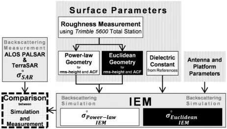
233 Figure 1 illustrates the flowchart of input parameters,
calculation, and finally comparison of results to evaluate the precision. The surface parameters along with the platform and antenna parameters were used to simulate the backscattering coefficient via two different inputs (computed using the Euclidean and the power-law geometries). By comparison, the simulated backscattering values were evaluated to provide the measured values of SAR backscattering.
In the shade of the irregular nature of the earth topography and consequently the irregular nature of the surface roughness parameters, estimations based on the fractal geometry could be biased by fewer errors in comparison with the one based on the Euclidean geometry. Unlike the Euclidean geometry shapes, fractals are not regular and are suitable for modeling the environmental effects (Falconer, 2004; Franceschetti, Iodice, Maddaluno, & Riccio, 2000; Mandelbrot, 1983).
These simulated results were compared to measure the backscattering coefficients of the SAR data on randomly selected points as the frequent evaluation procedure in the similar literature, e.g. (N. Baghdadi, Holah, & Zribi, 2006; Di Martino et al., 2014; Fernandez-Diaz, 2010; Franceschetti & Riccio, 2006).
Same as the general aim and methodology of this paper, other authors have proposed different approaches for implementation of fractal geometry to calculate the input geometric parameters of IEM mode (Ghafouri et al., 2017a; Ghafouri et al., 2017b) and the main contribution of this paper is to use Eqs. (6) and (7) to calculate the ACF.
In this paper, after introducing the IEM approach and the surface inputs calculation, its implementation on field measured data of the Zagros fold-thrust belt (in western Iran) is presented. To evaluate the results, the simulated values of the backscattering coefficient were compared with the SAR measured backscattering coefficient values. The results for both cases have been evaluated to assess the efficiency when using the power-law geometry in comparison with the Euclidean IEM.
2. IEM Backscattering Model
The value of co-polarized backscattering coefficients (i.e.
σhh° and σvv° ) or cross-polarized ones (i.e. σhv° or σvh° ) can be simulated Using the antenna and platform parameters, as well as the surface parameters, via the backscattering models (Ulaby & Long, 2014). The most famous model in this regard that is extensively used for co-polarized equations is the IEM (A.K. Fung, 1994; A. K. Fung & Chen, 2004; Adrian K Fung et al., 1992) (The interested readers are referred to (A. K. Fung & Chen, 2004) for a detailed review of the equations). Since the IEM was originally introduced, it has been modified by other researchers. The changes mostly concerned the approximations made in the original IEM; e.g.
Hsieh et al. (1997) proposed the IIEM, or Álvarez-Pérez
(2001) introduced the IEM2M, and the Advanced IEM (AIEM) was also created by Chen et al. (2003) (Álvarez-Pérez, 2001; Chen et al., 2003; Hsieh, Fung, Nesti, Sieber, & Coppo, 1997).
Researchers try to achieve the best possible model to correlate the backscattering coefficient and the surface parameters because the surface parameters can be estimated more precisely by having the SAR backscattering measurement. In this study, a higher precision was achieved using the IEM simulation and a more reliable surface morphology was estimated.
However, we assumed the improved version of the IEM for our study that was proposed by Ulaby & Long (2014) as I²EM, but preferably is called IEM in this manuscript. The geometric surface parameters are rms-height and ACF (A. K. Fung & Chen, 2004; Ulaby & Long, 2014). In the following two sections, two different methods of calculation for these parameters (i.e. Euclidean as well as fractal geometry) have been presented.
3. Euclidean Calculation of Surface Inputs
Considering the values of 𝑧𝑖 as the surface micro-topographic samples, rms-height as a statistical parameter should be calculated as (Dierking, 1999; Fernandez-Diaz, 2010) follows:
σ= √1
N[(∑zi2
N
i=1
) −Nz̅2] ∀z̅ =1
N∑zi
N
i=1
(1)
Normally, the exponential or Gaussian regression of the ACF is considered for calculation of W(n) in the model, as the
nth power of the surface power spectrum (Verhoest et al., 2008) which are respectively
ρ(ξ) =e-|ξ|⁄l (2)
ρ(ξ) =e-ξ
2
l2
⁄ (3)
where ξ is the correlation function variable parameter, 𝑙 is the correlation length calculated as one third of the semivariogram range (Western, Bloschl, & Grayson, 1998). The correlation length depends on the measurement profile length and can depend on the rms-height that can cause serious errors (Nicolas Baghdadi, Chaaya, & Zribi, 2011). Such dependency can be considered as the result of surface self-similarity and self-affinity. Considering the power-law geometry, one can avoid the errors significantly.
4. Power-law Calculation of the Surface Inputs
231 the ACF, can be calculated using the power-law parameters.
In this paper, the most distinguished ones, the fractal dimension (D) as well as Topothesy (τ), have been
considered as the fundamentals of calculation of both the rms-height and the ACF (Summers, Soukup, & Gragg, 2007).
We use the fractal dimension (D) for calculation of
σ=τ1-HLH (4)
where D=2-H in which D is the fractal dimension, τ is Topothesy, H is the Hurst parameter and L is the normal profile length. In this paper, the fractal dimension was calculated from the average slope of the regression line using the least squares method in the (log(∆x)).(log(∆h)) plot of the structural function (Vázquez, Miranda, & González, 2007; Mehrez Zribi, 1998). Having the Hurst exponent and the intercept of the straight line (a) of the RMS plot at the y-axis, the Topothesy can be calculated (Huang & Bradford, 1992).
τ= exp[(a
2-2H)] (5)
The Exponential and Gaussian correlation functions using the fractal dimension respectively are (6) and (7) (Mehrez Zribi, 1998)
𝜌(ξ) =l √π exp (-4 π2 ξ2 l2⁄ )4 (6)
𝜌(ξ) = 2l
1+4 π2ξ2l2 (7)
where, 𝜉 is spatial frequency and 𝑙, the correlation length. Spatial frequency is always smaller than the correlation length. The fractal calculation of correlation length is obtained through (8)
l=0.28 δ D+0.99 δ (8)
where δ is the profile sampling rate (Mehrez Zribi, 1998; M Zribi, Ciarletti, Taconet, Paillé, & Boissard, 2000).
Details of calculation of each parameter has been fully described in the aforementioned references.
5. The Case Study and Field Measurement
Due to the different geological formations and rocks of the Zagros fold-thrust belt, this region has been the subject of alteration investigation for long time (Aghanabati, 2004). Geologically, the Pabdeh (Paleocene to early Paleocene), Asmari (Lower Miocene), and Aghajari (Upper Miocene-Pliocene) geological formations have similar lithologies and their discrimination is not possible in areas having considerable topographic slope.
Because of having similar backscattering spectrums on hyperspectral images, separation of the upper boundary of the Pabdeh Formation and the lower boundary of the Asmari Formation is not easy and requires field visits; the same problem exists for both the Asmari and Aghajari formations (Figure 2). Using the SAR image processing, the number of geologists’ field visits reduces affectedly; hence, this method is one of the most efficient ways to provide the morphology information for the geological rock surfaces.
Figure 2. (a,b) The field view of the Asmari, Pabdeh, and Aghajari formations outcrop. Dashed lines separate the formations. Their difficult differentiation via hyperspectral satellite images leads to low accuracy of the geological formations maps. For the possible cases, this accuracy
can be improved via time-consuming field visits and adding morphological data
SE
NW SW
NE
Asmari Fm.
Pabdeh Fm.
Asmari Fm.
Aghajari Fm.
231 Figure 3. The case study location in western Iran as well as the three sites position on the Zagros thrust-fold belt
For this study, the SAR satellite images of ALOS PALSAR and TerraSAR as well as the geological map of 1: 50.000 and stratigraphic profiles of the area for the sites selection are used.
Three study sites for the three aforementioned geological formations are determined, and their micro-topography was measured for backscattering simulation using the Integral Equation Model (IEM). To evaluate the methodology implementation, the simulation results in each pixel was compared to the corresponding pixel values in measurement of SAR backscattering measurements. Figure 3 depicts the geological map of the region and the selected sites location.
Site1 on the Pabdeh Formation has a completely eroded structure and mostly appears in the form of soil on the terrain surface. The Pabdeh Formation (Pd) belongs to the Paleocene to early Miocene in age and separates the second and the third geologic periods. The cutting patterns in the north of Masjed-Soleyman has a thickness of 798m and consists of marl, limestone, and shale.
Site2 is located on the Asmari Formation and it is so much resistive against weathering and alteration, namely chemical and physical alterations. It has a rocky face. The Asmari Formation (As) is Oligocene to Lower Miocene in age. Its cutting patterns has a thickness of 314m and consists of cream to brown limestone with resistant morphological terrain.
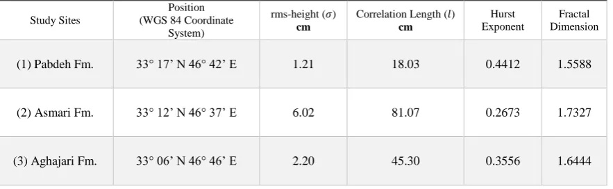
Site3 is situated on the Aghajari Formation. This site appears with a moderate situation in comparison with Sites 1 and 2; i.e. despite the presence of a rocky formation, the site is covered by rock fragments formed due to erosion and alterations. The Aghajari evaporitic formation (Aj) extends from the Dezful-Lorestan area to the Persian Gulf. In the northern part, it is the early Miocene in age and is a rock unit with a ductile behavior; therefore, it does not have a type locality at the ground level but a cutting pattern up to 1600m thick. Salt rock, anhydrite, colorful marl, limestone, and bitumen shale, without arranged folds, are the main units of the Aghajari formation. The geometric details of each site are presented in Table 1.
Table1. The study sites surface averaged geometric parameters
Study Sites
Position (WGS 84 Coordinate
System)
rms-height (𝜎)
cm
Correlation Length (𝑙)
cm
Hurst Exponent
Fractal Dimension
(1) Pabdeh Fm. 33° 17’ N 46° 42’ E 1.21 18.03 0.4412 1.5588
(2) Asmari Fm. 33° 12’ N 46° 37’ E 6.02 81.07 0.2673 1.7327
(3) Aghajari Fm. 33° 06’ N 46° 46’ E 2.20 45.30 0.3556 1.6444
Iraq Saudi Arabia Turkey Afghanistan Turkmenistan Pakistan Uzbekistan Syria Georgia Azerbaijan Russia Oman Untd Arab Em
Kazakhstan Armenia Tajikistan Qatar Jordan Kuwait 70°0'0"E 65°0'0"E 65°0'0"E 60°0'0"E 60°0'0"E 55°0'0"E 55°0'0"E 50°0'0"E 50°0'0"E 45°0'0"E 45°0'0"E 40°0'0"E 40°0'0"E 4 0 °0 '0 "N 4 0 °0 '0 "N 3 5 °0 '0 "N 3 5 °0 '0 "N 3 0 °0 '0 "N 3 0 °0 '0 "N 2 5 °0 '0 "N 2 5 °0 '0 "N 47°0'0"E 47°0'0"E 46°50'0"E 46°50'0"E 46°40'0"E 46°40'0"E 46°30'0"E 46°30'0"E 3 3 °2 0 '0 "N 3 3 °2 0 '0 "N 3 3 °1 0 '0 "N 3 3 °1 0 '0 "N 3 3 °0 '0 "N 3 3 °0 '0 "N Agha
jari Fm
. Pabdeh Fm.
Asmari Fm .
Asmari Fm. Asmari Fm.
Aghajari Fm. 2
1
3
▲
▲Case Study
1 Study Site
Caspian Sea
P e
r si a n
G u
l f
Oman Sea
231
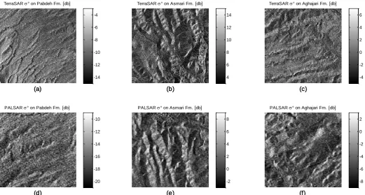
Figure 4. The backscattering coefficient on TerraSAR (a,b,c) and ALOS PALSAR (d,e,f) images of each geological formation of the sites; (a,d) Site1, Pabdeh Fm; (b,e) Site2, Asmari Fm; (c,f) Site3, Aghajarei Fm
Figure 4 depicts the measurement sites surface on the backscattering coefficient of the SAR images (ALOS PALSAR and TerraSAR, i.e. L-band and X-band, respectively) of the study area.
The IEM model and this article method implementation results require in-situ field measurements. Therefore, the surface roughness measurements in three sites were performed using the surveying Total station. Since the roughness parameters must be calculated along the linear profiles according to similar studies, the roughness parameters in this study were calculated as the average of several linear profiles on the site surface. Thus, field measurement in the form of a mesh of points make it possible to calculate the geometric parameters as the average of the multiple arbitrary profiles.
6. Implementation and Evaluation
In this section, the backscattering coefficient is simulated using the IEM for the antenna and platform of the two SAR images (i.e. TerraSAR as well as ALOS PALSAR) and the surface parameters (i.e. roughness and dielectric constant) of the three study sites. The surface roughness was measured and the dielectric constant was extracted from the references. The roughness in-situ measurement on the three field sites was performed using the surveying equipment, the Total Station. Also, the dielectric values for each geological formation were extracted from the Tables in Martinez & Byrnes (2001).
The surface roughness in situ measurement was performed using the programmable surveying Total Station
(Trimble™5600). This instrument has measured a 100×100 mesh with 50cm of interval on each measurement site. The measurement instrument has a one-centimeter better precision. Measuring as a mesh of points allows calculation of the roughness parameters along any arbitrary profile and certainly increases the precision of the parameters estimation.
The statistical rms-height (using Eq. (1)) as well as W(n) (i.e. nth Fourier transform of Eq. (2) and then Eq. (3)) were calculated to simulate the conventional IEM backscattering coefficient and having the dielectric constant of each site terrain, the value of 𝜎ℎℎ° and 𝜎𝑣𝑣° could be calculated as well.
Apart from this method, using Eq. (4), the rms-height can be calculated. Using Eq. (6) and Eq. (7), the ACF (and via its Fourier transform, the W(n)) can be achieved.
The surface roughness is needed for the morphological differentiation of the geological rock surfaces. Direct implementation of IEM model calculates the backscattering coefficient from the surface parameters for the certain platform and antenna.
In this paper, for assessment of the aforementioned calculation methods in Sections 3 and 4, it is necessary to compare the simulated backscattering coefficients using the IEM model with the measured values using the SAR images. For this comparison, the simulated and measured values for 30 selected pixels was compared on the point graphs. In addition, the standard deviations of the results were compared in tables as well as on bar charts.
TerraSAR ° on Pabdeh Fm. [db]
(a)
-14 -12 -10 -8 -6 -4
TerraSAR ° on Asmari Fm. [db]
(b)
4 6 8 10 12 14
TerraSAR ° on Aghajari Fm. [db]
(c)
-4 -2 0 2 4 6
PALSAR ° on Pabdeh Fm. [db]
(d)
-20 -18 -16 -14 -12 -10
PALSAR ° on Asmari Fm. [db]
(e)
-2 0 2 4 6 8
PALSAR ° on Aghajari Fm. [db]
(f)
231
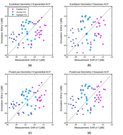
Figure 5. Backscattering coefficients simulation accuracy via the IEM model for the L-band compared with the measured backscattering coefficient values using ALOS PALSAR for the three geological formations, Pabdeh, Asmari, and Aghajari, (a) calculating the inputs via the
Euclidean geometry with the exponential ACF; (b) calculating the inputs via the Euclidean geometry with the Gaussian ACF; (c) calculating the inputs via the power-law geometry with the exponential ACF; (d) calculating the inputs via the power-law geometry with the Gaussian ACF
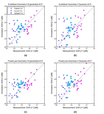
Comparisons between the backscattering coefficient values calculated through two Euclidean and two fractal methods of the geometric inputs calculation are presented for the three main geological formations in Figures 5 and 6, respectively for the L-band and the X-band. These plots demonstrate the IEM backscattering coefficient simulated values, “IEM Simulation”, compared to the satellite image, referred to as “SAR Measurement”. The L-band simulated values are compared with the ALOS PALSAR measurement and the X-band simulated values are compared with the
TerraSAR measurement. The smaller the standard deviation, the higher the accuracy of the simulated data.
Precisely being a point on the diagonal line of each graph indicates that the IEM model simulated backscattering coefficient on the corresponding pixel is exactly equal to the measured value on that pixel by the SAR. Evidently, for each graph, the proximity of simulated backscattering coefficient by the IEM model to the measured values from SAR image bears testimony to the improved performance in the method of the input parameters calculation in the model.
-30 -26 -22 -18 -14 -10
-30 -26 -22 -18 -14 -10
Measurement: SAR (°) [dB]
S
im
u
la
ti
o
n
:
IE
M
(
°)
[
d
B
]
Euclidean Geometry // Exponential ACF
(a) Pabdeh Fm. Asmari Fm. Aghajari Fm.
-30 -26 -22 -18 -14 -10
-30 -26 -22 -18 -14 -10
Measurement: SAR (°) [dB]
S
im
u
la
ti
o
n
:
IE
M
(
°)
[
d
B
]
Euclidean Geometry // Gaussian ACF
(b)
-30 -26 -22 -18 -14 -10
-30 -26 -22 -18 -14 -10
Measurement: SAR (°) [dB]
S
im
u
la
ti
o
n
:
IE
M
(
°)
[
d
B
]
PowerLaw Geometry // Exponential ACF
(c)
-30 -26 -22 -18 -14 -10
-30 -26 -22 -18 -14 -10
Measurement: SAR (°) [dB]
S
im
u
la
ti
o
n
:
IE
M
(
°)
[
d
B
]
PowerLaw Geometry // Gaussian ACF
231
Figure 6. Backscattering coefficients simulation accuracy via the IEM model for the X-band compared with the measured backscattering coefficient values using TerraSAR for the three geological formations, Pabdeh, Asmari, and Aghajari, (a) calculating the inputs via the Euclidean geometry with the exponential ACF; (b) calculating the inputs via the Euclidean geometry with the Gaussian ACF; (c) calculating the inputs via the power-law geometry with the exponential ACF; (d) calculating the inputs via the power-law geometry with the Gaussian ACF
In Table 2, the backscattering coefficient via the methods of IEM implementation are tabulated. In other words, the statistical dispersion of the simulated results on each site compared with SAR measured values, separately for each frequency, are depicted.
The values of the standard deviations show a general improvement for the IEM implementation results using the power-law geometry in comparison with the Euclidean geometry. However, with some fluctuations, this behavior has exceptions. The largest ratio of improvement that brings the power-law geometry in comparison with the Euclidean geometry is presented in the last column.
The Gaussian ACF for the Asmari and Aghajari formations leads to results that are more exact. This
performance for the both Euclidean and power-law geometry methods is noticeable. While the Gaussian ACF for the Pabdeh formation causes larger values of the standard deviation, better performance of implementation on the surface of this formation is perceptible for the Exponential ACF.
In case of power-law simulation, the simulated backscattering coefficient values for the Asmari and Aghajari formations on the L-band are close to ALOS PALSAR measured values. In addition, using the power-law simulation on the X-band, the simulated backscattering coefficients on the Pabdeh formation are more similar to TerraSAR measurement.
-25 -23 -21 -19 -17 -15
-25 -23 -21 -19 -17 -15
Measurement: SAR (°) [dB]
S
im
u
la
ti
o
n
:
IE
M
(
°)
[
d
B
]
Euclidean Geometry // Exponential ACF
(a) Pabdeh Fm. Asmari Fm. Aghajari Fm.
-25 -23 -21 -19 -17 -15
-25 -23 -21 -19 -17 -15
Measurement: SAR (°) [dB]
S
im
u
la
ti
o
n
:
IE
M
(
°)
[
d
B
]
Euclidean Geometry // Gaussian ACF
(b)
-25 -23 -21 -19 -17 -15
-25 -23 -21 -19 -17 -15
Measurement: SAR (°) [dB]
S
im
u
la
ti
o
n
:
IE
M
(
°)
[
d
B
]
PowerLaw Geometry // Exponential ACF
(c)
-25 -23 -21 -19 -17 -15
-25 -23 -21 -19 -17 -15
Measurement: SAR (°) [dB]
S
im
u
la
ti
o
n
:
IE
M
(
°)
[
d
B
]
PowerLaw Geometry // Gaussian ACF
231
Table2. Standard deviations of the simulated backscattering coefficient of the IEM model using four methods of implementing the IEM model, on the L and X frequency bands. Comparison between two different geometries is presented in the last column. The upper table shows the L-band simulated values being compared
with ALOS PALSAR measurement; The lower table presents the X-band simulated values being compared with TerraSAR measurement
Study Sites on L-band
Euclidean/ Exponential ACF
Euclidean/ Gaussian ACF
Power-law/ Exponential ACF
Power-law/ Gaussian ACF
Most Improvement
(1) Pabdeh Fm. 2.867 3.189 2.776 2.987 %6.8
(2) Asmari Fm. 2.01 1.822 1.56 1.706 %28.8
(3) Aghajari Fm. 2.664 2.562 2.291 2.505 %16.3
Study Sites on X-band
Euclidean/ Exponential ACF
Euclidean/ Gaussian ACF
Power-law/ Exponential ACF
Power-law/ Gaussian ACF
Most Improvement
(1) Pabdeh Fm. 0.843 1.065 0.696 0.927 %21.1
(2) Asmari Fm. 1.995 1.818 1.984 1.736 %4.7
(3) Aghajari Fm. 1.777 1.699 1.736 1.655 %2.6
Figure 7 illustrates the bar graph of the average simulated backscattering coefficient of the four methods in the implementation of IEM model for each frequency band. The closeness of the simulated values to the SAR measured values causes lower standard deviations which show the
improvement and effectiveness of the method of implementing the IEM model. On the graphs, the four methods for each geological formation in each SAR band are comparable.
Figure 7. The Bar chart of the standard deviation values presented in Table 2 of the simulated backscattering coefficient of the IEM model using four methods of implementing the IEM model for each geological formation; (a) for the L-band compared with ALOS PALSAR
measured values; (b) for the X-band compared with TerraSAR measured values
7. Discussion
In this paper, the Integral Equation Model (IEM) backscattering model was implemented for four different methods of input roughness parameters calculation. The four methods contain the exponential and the Gaussian ACFs in the Euclidean and power-law geometries. The IEM simulation results (i.e. backscattering coefficient values) were compared with SAR measurement. The L-band
simulated values were compared with ALOS PALSAR measurement whereas the X-band simulated values were compared with TerraSAR measurement.
Figures 5 and 6 show the values and give a visual sense of the results correctness. The numerical analysis of the results is presented via the standard deviation values in Table 2 and the bar-charts in Figure 7. In general, the fractal nature of the geological surface roughness yielded more efficiency
Pabdeh Asmari Aghajari
0 1 2 3 4 5
L-Band
2.867 3.189
2.776 2.987
2.01 1.822
1.56 1.706
2.664 2.562
2.291 2.505
(a)
Euclidean // Exp ACF Euclidean // Gau ACF PowerLaw // Exp ACF PowerLaw // Gau ACF
Pabdeh Asmari Aghajari
0 0.5 1 1.5 2 2.5
X-Band
0.843 1.065
0.696 0.927
1.995 1.818
1.984
1.736 1.777 1.699 1.736 1.655
211 of the power-law geometry versus the Euclidean geometry,
i.e. using the power-law geometry instead of the conventional form of the IEM backscattering model, the surface roughness is better distinguished. This improvement exhibits different effectiveness for different levels of roughness in different frequencies.
The Gaussian ACF for the rough rock surfaces results less deviation of simulation in comparison with the measurement. For smoother surfaces, the exponential ACF results in simulation that is more precise. This performance of the two ACF types is noticeable for both Euclidean and power-law geometry methods.
In case of power-law simulation, the simulated backscattering coefficient values for the rough surfaces at lower frequencies (e.g. L-band) are close to SAR measurement. Thus, it can be concluded that rough morphologies exhibit a fractal behavior at lower frequencies. If the power-law simulation is performed at higher frequencies (e.g. the X-band), rough morphologies have more diffractal regime and smoother morphologies are sensed to have a more fractal behavior. The simulated backscattering coefficients using the power-law geometry for smooth rock surfaces cause less deviation compared to SAR measurement.
8. Conclusion
This study investigated the application of random fractal geometry via implementation of the power-law geometry to improve the backscattering simulations of the Integral Equation Model (IEM) in description of geological rock surfaces. This study makes a significant contribution to the literature because the use of the fractal geometry is more representative than the Euclidean geometry of the irregular and fractal nature of natural surfaces. A comparative application to the terrain of the Zagros fold-thrust belt via ALOS PALSAAR and TerraSAR satellite data showed an evident improvement in the calculation of the geometric input parameters of the IEM for three different surface types. Although roughness modeling cannot be used as an independent mapping methodology, its implementation can help improve the traditional mapping methods and thus minimize the necessity for costly site visits and field measurement operations.
Somehow similar to the already published and cited publications of the authors, on each radar frequency, the specific size of the surface roughness can be measured via signal backscattering. Using two SAR bands L and X for the earth surface of three known-geological rock surfaces shows the capability of this technology in geological morphology mapping.
Application of random fractal geometry in the backscattering modeling offers more than 20% better results in the calculation of the surface geometry. However, the geometric behavior of the surface roughness against the SAR
frequencies is not constant, i.e. as micro-topography decreases, just in higher frequencies the fractal regime exists; contrariwise, smoother surfaces in lower frequencies are in a diffractal regime.
For this particular case study, although using the fractal geometry for the calculation of the inputs of IEM present an improvement, the improvement is less significant than the approaches which have been already published in the previous two papers, already mentioned in the introduction, and a comparative study should be performed to find the most effective method for other situations or applications.
Acknowledgement
The authors would like to thank the University Of Tehran Vice Chancellor Of Research for supporting this paper. Furthermore, we would like to acknowledge JAXA as well as DLR, the ALOS PALSAR and the TerraSAR-X program for providing the SAR data of the study area. Helpful comments and suggestions regarding the paper given by the respectful reviewers are acknowledged with gratitude.
References
Aghanabati, A. (2004). Geology of Iran: Geological Survey of Iran.
Álvarez-Pérez, J. L. (2001). An extension of the IEM/IEMM surface scattering model. Waves in Random Media, 11(3), 307-329.
Baghdadi, N., Chaaya, J. A., & Zribi, M. (2011). Semiempirical calibration of the integral equation model for SAR data in C-band and cross polarization using radar images and field measurements. Geoscience and Remote
Sensing Letters, IEEE, 8(1), 14-18.
Baghdadi, N., Holah, N., & Zribi, M. (2006). Calibration of the Integral Equation Model for SAR data in C‐ band and HH and VV polarizations. International Journal of
Remote Sensing, 27(4), 805-816.
doi:10.1080/01431160500212278
Chen, K.-S., Wu, T.-D., Tsang, L., Li, Q., Shi, J., & Fung, A. K. (2003). Emission of rough surfaces calculated by the integral equation method with comparison to three-dimensional moment method simulations. IEEE
Transactions on Geoscience and Remote Sensing, 41(1),
90-101.
Di Martino, G., Franceschetti, G., Iodice, A., Riccio, D., Ruello, G., & Zinno, I. (2014). Fractal dimension
estimation from fully polarimetric SAR data. Paper
presented at the Geoscience and Remote Sensing Symposium (IGARSS), 2014 IEEE International. Dierking, W. (1999). Quantitative roughness
characterization of geological surfaces and implications for radar signature analysis. Geoscience and Remote
Sensing, IEEE Transactions on, 37(5), 2397-2412.
Du, C., Yang, F., Xu, X., Xu, X., & Peng, M. (2014). Coal mine geological hazardous body detection using surface
ground penetrating radar velocity tomography. Paper
presented at the Ground Penetrating Radar (GPR), 2014 15th International Conference on.
Falconer, K. (2004). Fractal geometry: mathematical
212 Fernandez-Diaz, J. C. (2010). Characterization of surface
roughness of bare agricultural soils using LiDAR.
University of Florida.
Franceschetti, G., Iodice, A., Maddaluno, S., & Riccio, D. (2000). A fractal-based theoretical framework for retrieval of surface parameters from electromagnetic backscattering data. Geoscience and Remote Sensing,
IEEE Transactions on, 38(2), 641-650.
Franceschetti, G., & Riccio, D. (2006). Scattering, Natural
Surfaces, and Fractals: Academic Press.
Fung, A. K. (1994). Microwave Scattering and Emission
Models and Their Applications: Artech House.
Fung, A. K., & Chen, K. S. (2004). An update on the IEM surface backscattering model. Geoscience and Remote
Sensing Letters, IEEE, 1(2), 75-77.
doi:10.1109/LGRS.2004.826564
Fung, A. K., Li, Z., & Chen, K. (1992). Backscattering from a randomly rough dielectric surface. Geoscience and
Remote Sensing, IEEE Transactions on, 30(2).
Ghafouri, A. (2017). Top-Geological Formations Surface
RoughnessModeling in SAR Image. School of Surveying
and Geospatial Engineering, Faculty of Engineering, University of Tehran, Iran, PhD. Thesis.
Ghafouri, A., Amini, J., Dehmollaian, M., & Kavoosi, M. (2015). Random Fractals Geometry in Surface Roughness Modeling of Geological Formations using Synthetic Aperture Radar Images. Journal of Geomatics Science and Technology, Iranian Society for Surveying &
Geomatics Engineering, 5(2), 97-108.
Ghafouri, A., Amini, J., Dehmollaian, M., & Kavoosi, M. (2017a). Measuring Surface Roughness of Geological Rock Surfaces in SAR Data using Fractal Geometry.
Comptes Rendues Geosciences.
Ghafouri, A., Amini, J., Dehmollaian, M., & Kavoosi, M. A. (2017b). Better Estimated IEM Input Parameters Using Random Fractal Geometry Applied on Multi-Frequency SAR Data. Remote Sensing, 9(5), 445.
Hsieh, C.-Y., Fung, A. K., Nesti, G., Sieber, A. J., & Coppo, P. (1997). A further study of the IEM surface scattering model. IEEE Transactions on Geoscience and Remote
Sensing, 35(4), 901-909.
Huang, C.-h., & Bradford, J. M. (1992). Applications of a Laser Scanner to Quantify Soil Microtopography. Soil
Science Society of America Journal, 56(1).
doi:10.2136/sssaj1992.03615995005600010002x Iodice, A., Natale, A., & Riccio, D. (2013). Kirchhoff
scattering from fractal and classical rough surfaces: Physical interpretation. Antennas and Propagation, IEEE
Transactions on, 61(4), 2156-2163.
Irena, H. (2001). Inversion of surface parameters using
Polarimetric SAR. Ph. D. thesis, 2001, Germany.
Li, Z., Yang, R., Dang, F., Du, P., Zhang, X., Tan, B., Su, H. (2012, 4-7 June 2012). A review on the geological applications of hyperspectral remote sensing technology.
Paper presented at the Hyperspectral Image and Signal Processing: Evolution in Remote Sensing (WHISPERS), 2012 4th Workshop on.
Lutgens, F. K. (2006). Essentials of Geology/FREDERICK
LUTGENS, EDWARD J. TARBUCK.
Mandelbrot, B. B. (1983). The fractal geometry of nature
(Vol. 173): Macmillan.
Martinez, A., & Byrnes, A. P. (2001). Modeling dielectric-constant values of geologic materials: An aid to
ground-penetrating radar data collection and interpretation:
Kansas Geological Survey, University of Kansas. Martino, G. D., Iodice, A., Riccio, D., & Ruello, G. (2010).
Imaging of fractal profiles. Geoscience and Remote
Sensing, IEEE Transactions on, 48(8), 3280-3289.
Motiei, H. (1993). Stratigraphy of Zagros. Treatise on the
Geology of Iran(1), 60-151.
Summers, J. E., Soukup, R. J., & Gragg, R. F. (2007). Mathematical modeling and computer-aided manufacturing of rough surfaces for experimental study of seafloor scattering. Oceanic Engineering, IEEE
Journal of, 32(4), 897-914.
Ulaby, F. T., & Long, D. G. (2014). Microwave Radar and Radiometric Remote Sensing. 425-445.
Vázquez, E. V., Miranda, J., & González, A. P. (2007). Describing soil surface microrelief by crossover length and fractal dimension. Nonlinear Processes in
Geophysics, 14(3), 223-235.
Verhoest, N. E., Lievens, H., Wagner, W., Álvarez-Mozos, J., Moran, M. S., & Mattia, F. (2008). On the soil roughness parameterization problem in soil moisture retrieval of bare surfaces from synthetic aperture radar.
Sensors, 8(7), 4213-4248.
Western, A. W., Bloschl, G., & Grayson, R. B. (1998). How well do indicator variograms capture the spatial connectivity of soil moisture? Hydrological processes, 12(12), 1851-1868.
Zribi, M. (1998). Développement de nouvelles méthodes de modélisation de la rugosité pour la rétrodiffusion
hyperfréquence de la surface du sol.
Zribi, M., Ciarletti, V., Taconet, O., Paillé, J., & Boissard, P. (2000). Characterisation of the soil structure and microwave backscattering based on numerical three-dimensional surface representation: Analysis with a fractional brownian model. Remote sensing of