Regularities

NBER WORKING PAPER SERIES

REGULARITIES

Laura X. L. Liu

Toni Whited

Lu Zhang

Working Paper 13024

http://www.nber.org/papers/w13024

NATIONAL BUREAU OF ECONOMIC RESEARCH

1050 Massachusetts Avenue

Cambridge, MA 02138

April 2007

We thank Nick Barberis, David Brown, V. V. Chari, Rick Green, Burton Hollifield, Patrick Kehoe,

Narayana Kocherlakota, Leonid Kogan, Owen Lamont, Sydney Ludvigson, Ellen McGrattan, Antonio

Mello, Mark Ready, Bryan Routledge, Martin Schneider, Masako Ueda, and seminar participants at

the Federal Reserve Bank of Minneapolis, Yale School of Management, University of Wisconsin--Madison,

Carnegie-Mellon University, New York University, Society of Economic Dynamics Annual Meetings

in 2006, the UBC Summer Finance Conference in 2006, and the American Finance Association Annual

Meetings in 2007 for helpful comments. Some of the theoretical results have previously been circulated

in NBER working paper #11322 titled "Anomalies.'' All remaining errors are our own. The views expressed

herein are those of the author(s) and do not necessarily reflect the views of the National Bureau of

Economic Research.

© 2007 by Laura X. L. Liu, Toni Whited, and Lu Zhang. All rights reserved. Short sections of text,

not to exceed two paragraphs, may be quoted without explicit permission provided that full credit,

Regularities

Laura X. L. Liu, Toni Whited, and Lu Zhang

NBER Working Paper No. 13024

April 2007

JEL No. E13,E22,E44,G12

ABSTRACT

The neoclassical q-theory is a good start to understand the cross section of returns. Under constant

return to scale, stock returns equal levered investment returns that are tied directly with characteristics.

This equation generates the relations of average returns with book-to-market, investment, and earnings

surprises. We estimate the model by minimizing the differences between average stock returns and

average levered investment returns via GMM. Our model captures well the average returns of portfolios

sorted on capital investment and on size and book-to-market, including the small-stock value premium.

Our model is also partially successful in capturing the post-earnings-announcement drift and its higher

magnitude in small firms.

Laura X. L. Liu

Finance Department

School of Business and Management

Hong Kong University of

Science and Technology

Kowloon, Hong Kong

[email protected]

Toni Whited

University of Wisconsin

Finance Department

975 University Avenue

Madison, WI 53706

[email protected]

Lu Zhang

Finance Department

Stephen M. Ross School of Business

University of Michigan

701 Tappan Street, ER 7605 Bus Ad

Ann Arbor MI, 48109-1234

and NBER

1

Introduction

The empirical finance literature has documented tantalizing relations between future stock returns and firm characteristics. As surveyed in, for example, Fama (1998) and Schwert (2003), traditional asset pricing models have failed to explain many of these relations, which have therefore been dubbed anomalies. Several prominent studies, such as Shleifer (2000) and Barberis and Thaler (2003), have interpreted this failure as prima facia evidence against the efficient markets hypothesis. We use the neoclassical q-theory of investment to provide the microfoundation for time-varying expected returns in the cross section, thus providing a structural framework for understanding the anomalies and for capturing them empirically. As first shown by Cochrane (1991), under con-stant return to scale, stock returns equal investment returns, which are tied to firm characteristics through the optimality conditions of investment. We use these conditions to show how expected returns vary in the cross section with firm characteristics, corporate policies, and events.

We show that the q-theory can generate the following anomalies. The first is the investment anomaly: The investment-to-assets ratio is negatively correlated with average returns. The second is the value anomaly: Value stocks (with high book-to-market ratios) earn higher average returns than growth stocks (with low book-to-market ratios), especially for small firms. The third is the post-earnings-announcement drift anomaly: Firms with positive earnings surprises earn higher av-erage returns than firms with negative earnings surprises, especially for small firms.

The intuition behind the way in which the q-theory generates these anomalies is most trans-parent in a simple two-period example. The investment return from timetto t+ 1 equals the ratio of the marginal profit of investment att+ 1 divided by the marginal cost of investment att. This definition implies two economic forces driving asset pricing anomalies. First, optimal investment produces a negative relation between investment and expected returns. The ratio of investment to assets increases with the net present value of capital, and the net present value decreases with the cost of capital or the expected return. The investment anomaly occurs because a low cost of capital implies high net present value, which in turn implies high investment. The value anomaly results from the same driving force because investment is an increasing function of marginal q, which is closely linked to the market-to-book ratio. The negative investment-return relation then implies a negative relation between market-to-book and expected returns.

Whereas the first driver operates through the denominator of the investment return, the second operates through the numerator. The marginal product of capital at time t+ 1 in the numerator

of the investment return equation drives post-earnings-announcement drift in our model. Under constant return to scale, the marginal product of capital equals the average product of capital, which in turn equals profitability plus the rate of capital depreciation. This link suggests a positive relation between expected profitability and expected returns, all else equal. Because profitability is highly persistent and because earnings surprises are positively correlated with profitability, our model therefore predicts that earnings surprises are positively correlated with expected returns.

Intriguingly, our economic explanations of anomalies do not involve risk directly, even though we do not assume overreaction or underreaction, as in Daniel, Hirshleifer, and Subrahmanyam (1998). Because we derive expected returns from the optimality conditions of firms, the stochastic discount factor and its covariance with stock returns do not enter the expected-return determination, at least directly. Characteristics are sufficient statistics for expected returns, even in efficient markets. This result clearly helps interpret the debate on covariances versus characteristics in empirical finance in, for example, Daniel and Titman (1997) and Davis, Fama, and French (2000).

Although intuitively compelling, our economic mechanisms are but curiosities unless they can be upheld by data. We therefore test empirically whether theq-theory can quantitatively capture asset pricing anomalies. We test a purely characteristics-based expected return model derived from the dynamic value maximization problem underlying the q-theory. To facilitate empirical tests of the theory, we derive new analytical relations between stock and investment returns after incorpo-rating flow opeincorpo-rating costs, leverage, and financing costs of external equity. We then use GMM to minimize the differences between the average stock returns observed in the data and the expected stock returns implied by the model. Our data comprise several sets of testing portfolios designed to capture cross sectional variations of average returns. We examine the value anomaly in the Fama-French (1993) 25 size and book-to-market portfolios, the post-earnings-announcement drift in ten portfolios sorted by Standardized Unexpected Earnings (SUE), and the negative relation between expected returns and investment in ten portfolios sorted by the ratio of investment to assets and in ten portfolios sorted by the abnormal investment measure of Titman, Wei, and Xie (2004).

The q-theoretic mechanisms are empirically important. Average stock returns in the data and model-implied expected returns track each other closely across portfolios sorted by investment and across portfolios sorted by size and book-to-market. When we apply the benchmark model with only physical adjustment costs to the Fama-French (1993) 25 portfolios (a task comparable to that of Fama and French, 1996, Table I), the average absolute pricing error is only 7.4 basis points per

month. The overidentification test fails to reject the null hypothesis that the average pricing error is zero. Further, none of the 25 alphas are significantly different from zero. The small-stock value strategy, in particular, carries a negligible alpha of 4 basis points per month.

The model performance is more modest in matching average returns across the SUE portfolios. When we only use the SUE portfolios in the moment conditions, the benchmark model generates an average difference of 0.91% per month between the returns of the low and high SUE portfolios, but the extreme deciles have significant alphas of −0.21% and −0.36% per month, respectively. The model also performs well for the nine double-sorted size and SUE portfolios. In particular, the model-implied average return spread between the low SUE and high SUE terciles is 0.80% per month in small firms, a difference noticeably higher than the 0.14% per month difference in big firms. Unfortunately, the difference in model-implied average returns between extreme SUE portfolios largely disappears in joint estimation, in which we also ask the model to price all the other testing portfolios simultaneously.

Our asset pricing approach represents a fundamental departure from traditional approaches in the cross section of returns. Derived from optimality conditions, our approach differs from empir-ically motivated factor models, as in Fama and French (1993, 1996). In contrast to consumption-based asset pricing (e.g., Hansen and Singleton 1982, Lettau and Ludvigson 2001), our Euler equa-tion tests do not use informaequa-tion on preferences. Our expected return model is based entirely on firm characteristics. In view of the empirical difficulty in estimating risk and risk premia documented in, for example, Fama and French (1997), it is perhaps not surprising that our model outperforms traditional asset pricing models in capturing anomalies. As noted, unlike behavioral approach as in Daniel, Hirshleifer, and Subrahmanyam (1998), the expectations in our model are all rational ex-pectations. Differing further from behavioral studies, we propose and test a new structural expected return model using rational expectations econometrics `a la Hansen and Sargent (1991).

Our approach builds on Cochrane (1991), who establishes the link between stock and investment returns. Cochrane (1996) uses aggregate investment returns to price the cross section, and Cochrane (1997) uses the investment-return equation to address the equity premium puzzle. Lettau and Lud-vigson (2002) explore the implications of time-varying risk premia on aggregate investment growth in theq-theoretic framework. We contribute by employing theq-theory to address anomalies in the cross section. We also add to studies of the cross section of returns based on dynamic optimization of firms, as in Berk, Green, and Naik (1999), Carlson, Fisher, and Giammarino (2004), and Zhang

(2005). Our work differs because we do structural estimation on closed-form estimating equations. Our work is also related to theq-theory of investment originated by Brainard and Tobin (1968) and Tobin (1969). Theoretically, the equivalence between stock and investment returns is an alge-braic restatement of the equivalence between marginalq and averageq, demonstrated in Lucas and Prescott (1971), Hayashi (1982), and Abel and Eberly (1994). Empirically, our work is connected to investment Euler equation tests designed to understand investment behavior, for example, Shapiro (1986) and Whited (1992). We extend this approach by restating the investment Euler equation in terms of stock returns and testing it with data on the cross section of returns.

2

A Two-Period Example

We use a simple two-period example that follows Cochrane (1991, 1996) to provide intuition behind the link between expected returns and firm characteristics.

2.1 The Setup

Firms use capital and a vector of costlessly adjustable inputs to produce a perishable output good. Firms choose the levels of these inputs each period to maximize their operating profits, defined as revenues minus the expenditures on these inputs. Taking the operating profits as given, firms then choose optimal investment to maximize their market value.

There are only two periods, tand t+ 1. Firm j starts with capital stock kjt, invests in period

t, and produces in both t and t+ 1. The firm exits at the end of period t+ 1 with a liquida-tion value of (1−δj)kjt+1, in which δj is the firm-specific rate of capital depreciation. Operating profits, πjt=π(kjt, xjt), depend upon capital, kjt, and a vector of exogenous aggregate and firm-specific productivity shocks, denoted xjt. Operating profits exhibit constant return to scale, that is, π(kjt, xjt) = π1(kjt, xjt)kjt, in which numerical subscripts denote partial derivatives. The ex-pressionπ1(kjt, xjt) is therefore the marginal product of capital.

The law of motion for capital is kjt+1 = ijt+ (1−δj)kjt, in which ijt denotes capital invest-ment. We use the one-period time-to-build convention: Capital goods invested today only become productive at the beginning of next period. Investment incurs quadratic adjustment costs given by (a/2)(ijt/kjt)2kjt, in which a > 0 is a constant parameter. The adjustment-cost function is increasing and convex inijt, decreasing inkjt, and exhibits constant return to scale.

Let mt+1 be the stochastic discount factor from time t to t+ 1, which is correlated with the aggregate component of xjt+1. Firmj chooses ijt to maximize the market value of equity:

max {ijt}         

Cash flow at periodt

z }| { π(kjt, xjt)−ijt− a 2 ijt kjt 2 kjt+Et   mt+1   

Cash flow at period t+1

z }| { π(kjt+1, xjt+1) + (1−δj)kjt+1                | {z }

Cumulative dividend market value of equity at periodt

. (1)

The first part of this expression, denoted by π(kjt, xjt)−ijt−(a/2)(ijt/kjt)2kjt, is net cash flow during periodt. Firms use operating profitsπ(kjt, xjt) to invest, which incurs both purchase costs,

ijt, and adjustment costs, (a/2) (ijt/kjt)2kjt. The price of capital is normalized to be one. If net cash flow is positive, firms distribute it to shareholders, and if net cash flow is negative, firms collect external equity financing from shareholders. The second part of equation (1) contains the expected discounted value of cash flow during period t+ 1, which is given by the sum of operating profits and the liquidation value of the capital stock at the end oft+ 1.

Taking the partial derivative of equation (1) with respect to ijtyields the first-order condition: Marginal cost of investment at period t

z }| { 1 +a ijt kjt = Et   mt+1   

Marginal benefit of investment at periodt+1

z }| { π1(kjt+1, xjt+1) + (1−δj)      . (2)

The left side of (2) is the marginal cost of investment, and the right side is the marginal benefit. To generate one additional unit of capital at the beginning of next period, kjt+1, firms must pay the price of capital and the marginal adjustment cost,a(ijt/kjt). The next-period marginal benefit of this additional unit of capital includes the marginal product of capital,π1(kjt+1, xjt+1), and the liquidation value of capital net of depreciation, 1−δj. Discounting this next-period benefit using the pricing kernelmt+1 yields a quantity commonly dubbed marginal q. More precisely,

qjt≡Et[mt+1(π1(kjt+1, xjt+1) + (1−δj))].

To derive asset pricing implications from this two-period q-theoretic model, we first define the investment return as the ratio of the marginal benefit of investment at periodt+ 1 divided by the

marginal cost of investment at periodt:

r_jtI+1

| {z }

Investment return from period tto t+1

≡

Marginal benefit of investment at periodt+1

z }| {

π1(kjt+1, xjt+1) + (1−δj) 1 +a(ijt/kjt)

| {z }

Marginal cost of investment at periodt

(3)

Following Cochrane (1991), we divide both sides of equation (2) by the marginal cost of investment:

Et

mt+1rI_jt+1

= 1.

We now show that under constant return to scale, stock returns equal investment returns. From equation (1) we define the ex-dividend equity value at period t, denotedpjt, as:

pjt

|{z}

Ex dividend equity value at periodt

= Et   mt+1   

Cash flow at period t+1

z }| { π(kjt+1, xjt+1) + (1−δj)kjt+1      , (4) The ex-dividend equity value,pjt, equals the cum-dividend equity value—the maximum in equation (1)—minus the net cash flow over periodt. We can now define the stock return,rS

jt+1,as

r_jtS+1

| {z }

Stock return from periodttot+1 =

Cash flow at period t+1

z }| {

π(kjt+1, xjt+1) + (1−δj)kjt+1

Et[mt+1[π(kjt+1, xjt+1) + (1−δj)kjt+1]]

| {z }

Ex dividend equity value at periodt

, (5)

in which the ex-dividend market value of equity in the numerator is zero in this two-period setting. Dividing both the numerator and the denominator of equation (5) by kjt+1, and invoking the constant returns assumption yields:

r_jtS+1= π1(kjt+1, xjt+1) + (1−δj) Et[mt+1[π1(kjt+1, xjt+1) + (1−δj)]] = π1(kjt+1, xjt+1) + (1−δj) 1 +a(ijt/kjt) =r_jtI+1.

The second equality follows from the first-order condition given by equation (2). Because of this equivalence, in what follows, we use rjt+1 to denote both stock and investment returns.

2.2 Intuition

We use the equivalence between stock and investment returns to provide economic intuition about the driving forces behind expected returns:

Et[rjt+1]

| {z }

Expected return =

Expected marginal product of capital

z }| {

Et[π1(kjt+1, xjt+1)] + 1−δj 1 +a(ijt/kjt)

| {z }

Marginal cost of investment

. (6)

Justification for this approach is in Cochrane (1997), who shows that average aggregate equity returns are well within the range of plausible parameters for average aggregate investment returns. Equation (6) is useful for interpreting anomalies because it ties expected returns directly to firm characteristics. The equation implies that there are two channels through which firm characteristics can affect expected returns. The investment-to-assets ratio,ijt/kjt, affects expected returns through the discount-rate channel, and the expected marginal product of capital,Et[π1(kjt+1, xjt+1)] affects expected returns through the cash-flow channel. We discuss each below.

The Investment and Value Anomalies: The Discount-Rate Channel

Holding constant the expected marginal product of capital and the rate of capital depreciation, equation (6) implies the negative relation between expected returns and investment-to-assets, as in Cochrane (1991). In the capital budgeting language of Brealey, Myers, and Allen (2006, Chapter 6), investment-to-assets increases with the net present value of capital. All else equal, the net present value decreases with the cost of capital, which is precisely the expected return. Given expected cash flows, a high cost of capital implies a low net present value, which in turn implies a low investment-to-assets ratio. Conversely, a low cost of capital implies a high net present value, which in turn implies a high investment-to-assets ratio. Figure 1 illustrates the negative relation between investment-to-assets and expected returns.

Adjustment costs are a crucial ingredient for the discount-rate channel. Equation (6) implies that, without adjustment costs (a= 0), expected returns are independent of investment-to-assets.1

1_{Formally, ∂Et[r}

jt+1]/∂(ijt/kjt) = −a(Et[π1(kjt+1, xjt+1)] + 1−δj)/[1 +a(ijt/kjt)]2 < 0. When a = 0,

∂Et[rjt+1]/∂(ijt/kjt) = 0. More precisely, because of kjt+1 = [ijt/kjt+ (1−δj)]kjt, we also should worry about

the effect of investment at periodton the capital stock at the beginning of periodt+1. Letπ11(kjt+1, xjt+1) denote

the second order partial derivative ofπ(kjt+1, xjt+1) with respect tokjt+1. We have:

∂Et[rjt+1] ∂(ijt/kjt) =− a(Et[π1(kjt+1, xjt+1)] + 1−δj) [1 +a(ijt/kjt)]2 +Et[π11(kjt+1, xjt+1)kjt] 1 +a(ijt/kjt) =− a(Et[π1(kjt+1, xjt+1)] + 1−δj) [1 +a(ijt/kjt)]2

Figure 1 also shows that growth firms have low expected returns and that value firms have high expected returns. This pattern follows directly from a one-to-one mapping between the investment-to-assets ratio and the market-to-book ratio. The mapping implies that growth firms invest more and earn lower expected returns, and that value firms invest less and earn higher expected returns. To derive this mapping, we define average Q, denotedQjt, as pjt/kjt+1. We then divide equation (4) bykjt+1 and use equation (2) to obtain the equality of marginalq and average Q:

1 +a ijt kjt =qjt=Qjt≡ pjt kjt+1 . (7)

Equation (7) implies that∂(ijt/kjt)/∂Qjt= 1/a >0, which says that growth firms with high market-to-book ratios invest more than value firms with low market-market-to-book ratios (e.g., Fama and French 1995; Xing 2006). The value anomaly follows because:

∂Et[rjt+1] ∂Qjt = ∂Et[r S jt+1] ∂(ijt/kjt) ∂(ijt/kjt) ∂Qjt <0.

The investment-return relation is convex.2

Moreover, ∂(ijt/kjt)/∂pjt>0, which again means that highQfirms invest more than lowQfirms, and which follows because equation (7) implies that

pjt= [1+a(ijt/kjt)](ijt/kjt+1−δ)kjtand∂pjt/∂(ijt/kjt) =qjtkjt+akjt+1 >0.3 The chain rule com-bines the convexity with∂(ijt/kjt)/∂pjt>0 to generate the stronger value anomaly in small firms.4

The Post-Earnings-Announcement Drift: The Cash-Flow Channel

The relation between earnings and average returns arises naturally in our neoclassical model. In-tuitively, the marginal product of capital in the numerator of the expected-return equation (6) is closely related to earnings. Accordingly, expected returns increase with earnings.

The earnings-return relation persists even without capital adjustment costs. In this sense, the earnings-return relation is more fundamental than the investment-return relation and the

value-the assumption of decreasing returns to scale reinforces our result becauseπ11(kjt+1, xjt+1)<0.

2_{The convexity follows from∂}2_Et[r

jt+1]/∂(ijt/kjt)2= 2a2(Et[π1(kjt+1, xjt+1)] + 1−δj)/[1 +a(ijt/kjt)]3>0.

3_∂p

jt/∂(ijt/kjt)>0 does not imply that big firms invest more than small firms. Although firm size means market

capitalization in empirical finance (e.g., Fama and French 1993), firm size means physical size in macroeconomics and in our model. Evans (1987) and Hall (1987) show that small firms invest more and grow faster than big firms,

using the logarithm of employment as the measure of firm size. The measure corresponds to log(kjt) in our model.

More importantly, from equation (2). ijt/kjt is independent ofkjtin our model (constant return to scale).

4_{More precisely, ∂}˛˛ ˛ ∂Et[rjt+1] ∂Qjt ˛ ˛ ˛/∂pjt =− ∂2_E t[rjt+1] ∂Qjt∂pjt =− 1 a ∂2_E t[rjt+1] ∂(ijt/kjt)2 ∂(ijt/kjt)

∂pjt < 0,in which the second equality

return relation. Specifically, whena= 0, equation (6) reduces to:

Et[rjt+1]

| {z }

Expected return =

Expected marginal product of capital

z }| {

Et[π1(kjt+1, xjt+1)] + 1−δj . (8)

The expected (net) return equals the expected marginal product of capital minus the depreciation rate. Earnings equals operating cash flows minus capital depreciation, which is the only accrual in our model.5 _{Let e}

jt denotes earnings, then:

ejt

|{z}

Earnings

≡

Operating cash flows

z }| {

π(kjt, xjt) − δjkjt

| {z }

Capital depreciation

. (9)

We can now link expected returns to expected profitability by using constant return to scale and equation (9) to rewrite equation (8) as:

Et[rjt+1]

| {z }

Expected return =

Average product of capital

z }| { Et πjt+1 kjt+1 + 1−δj = Et ejt+1 kjt+1 | {z } Expected profitability + 1. (10)

Equation (10) states that expected returns equal expected profitability.

To link expected returns further to earnings surprises, we note that profitability is highly per-sistent.6

Suppose profitability follows an autoregressive process given by:

ejt+1 kjt+1 = ¯e(1−ρe) + ρe ejt kjt | {z } Expected profitability + Earnings surprise z }| { εe_jt+1 (11)

in which ¯eand 0< ρ_e<1 are the long-run average and the persistence of profitability, respectively, and in whichεe

jt+1 denotes the earnings surprise. The term ¯e(1−ρe)+ρe(ejt/kjt) therefore denotes expected profitability. Combining equations (10) and (11) yields:

Et[rjt+1] | {z } Expected return = e¯(1−ρe) + ρe Profitability z }| { ejt kjt | {z } Expected profitability + 1 (12)

5_{We assume implicitly that there is no accounting timing and matching problem that causes operating cash flows}

to deviate from earnings (e.g., Dechow 1994). In particular, we do not model earnings management.

6_{There is much evidence on the persistence in profitability at the portfolio level and at the firm level (e.g., Fama}

and French 1995, 2000, 2006). For example, Fama and French (2006) document that the current-period profitability is the strongest predictor of profitability one to three years ahead.

Expected returns thus increase with the current-period profitability. This insight only depends on the persistence in profitability, not the specific functional form in equation (11).

Plugging the one-period-lagged equation (11) into equation (12) yields:

Et[rjt+1] | {z } Expected return = e¯(1−ρ_e)(1 +ρ_e) +ρ2_e ejt−1 kjt−1 + ρ_e Earnings surprise z}|{ εe_t | {z } Expected profitability + 1 (13)

Expected returns have a positive loading, ρ_e, on earnings surprises, εe

t. The magnitude of the post-earnings-announcement drift increases with the average persistence in firm-level profitability. However, equation (13) predicts that the magnitude of the post-earnings-announcement drift is constant across different market capitalization groups. To generate a stronger magnitude in small firms, we add adjustment costs back to the model. Combining equations (6) and (9) yields:

Et[rjt+1] | {z } Expected return = Expected profitability z }| { Et[ejt+1/kjt+1] + 1 1 +a(ijt/kjt) | {z }

Marginal cost of investment

(14)

Therefore, controlling for the denominator, which by equation (7) equals market-to-book, equation (14) predicts that expected returns increase with expected profitability.7

From equation (14), high profitability relative to market-to-book allows us to infer high discount rate. Because we do not model overreaction and underreaction, high discount rate follows from high risk (see Section 4.1 below for more discussion on this point). Our firm-centered perspective there-fore allows us to infer unobservable risk and expected returns from observable firm characteristics. More intriguingly, equation (14) implies that the loading of expected returns on the expected profitability equals 1/Qjt=kjt+1/pjt, which is inversely related to market capitalization,pjt.8 This is consistent with Cohen, Gompers, and Vuolteenaho’s (2002) evidence that the relation between expected profitability and average returns is stronger in small firms.

7_{Empirically, Haugen and Baker (1996) and Fama and French (2006) show that, controlling for market valuation}

ratios, firms with high expected profitability earn higher average returns than firms with low expected profitability.

8_{Fama and French (1992) document that the average cross-sectional correlation between book-to-market and}

Moreover, combining equations (6) and (9) yields: Et[rjt+1] | {z } Expected return = Expected profitability z }| { ¯ e(1−ρe)(1 +ρe) +ρ 2 e(ejt−1/kjt−1) + ρ_e εe_t |{z} Earnings surprise + 1 1 +a(ijt/kjt) | {z }

Marginal cost of investment

(15)

Controlling for market-to-book, we have expected returns increase with earnings surprises, and the loading of expected returns on earnings surprises equals ρekjt+1/pjt, which is inversely related to market capitalization, pjt. This prediction is consistent with the Bernard and Thomas (1989) evidence that the magnitude of the post-earnings-announcement drift is higher in small firms.

3

Dynamic Models

We present two models: the all-equity model (Section 3.1) and the leverage model (Section 3.2). We also consider a more technically complex model with costly external equity in Appendix D.

3.1 The All-Equity Model

Time is discrete and the horizon infinite. Firms use capital and a vector of costlessly adjustable inputs to produce a homogeneous output. The levels of these inputs are chosen each period to max-imize operating profits, defined as revenues minus the expenditures on these inputs. Taking the operating profits as given, firms then choose optimal investment to maximize their market value. As in the two-period model πjt≡π(kjt, xjt) denotes the maximized operating profits of firm j at time t, and π(kjt, xjt) exhibits constant return to scale. End-of-period capital equals investment plus beginning-of-period capital net of depreciation:

kjt+1=ijt+ (1−δjt)kjt (16)

We assume that capital depreciates at an exogenous proportional rate of δjt. This rate is firm-specific and time-varying because we use data on capital depreciation divided by capital stock to measure the rate of depreciation later in our tests. Also, as in the two-period model, firms incur ad-justment costs when they invest. However, we now specify the adad-justment cost function,φ(ijt, kjt) as capturing both purchase/sale costs and physical adjustment costs. The function φ(ijt, kjt) sat-isfies φ1 ≤ 0, φ2 ≤0, and φ11 >0. Another important ingredient is a flow operating cost. Firms that stay in production each period must incur a flow operating cost proportional to capital stock,

ckjt, in which the parameterc >0 is a constant common to all firms.

Let qjt be the present-value multiplier associated with equation (16). We can formulate the market value of firmj, denoted v(kjt, xjt), as follows:

v(kjt, xjt) = max {ijt+τ, kjt+1+τ}∞τ=0 Et "_∞ X τ=0 mt+τ[π(kjt+τ, xjt+τ)−ckjt+τ−φ(ijt+τ, kjt+τ) −qjt+τ[kjt+τ+1−(1−δjt+τ)kjt+τ −ijt+τ]] # . (17) The first-order conditions with respect to ijt and kjt+1 are, respectively,

qjt = φ1(ijt, kjt), (18)

qjt = Et[mt+1(π1(kjt+1, xjt+1)−c−φ2(ijt+1, kjt+1) + (1−δjt+1)qjt+1)]. (19)

Equation (18) is the optimality condition for investment that equates the marginal cost of investing,

φ1(ijt, kjt), with its marginal benefit,qjt, which is the shadow value of capital or, equivalently, the expected present value of the marginal profits from investing in capital goods. Equation (19) is the Euler condition that describes the evolution of qjt.Combining equations (18) and (19) yields:

φ1(ijt, kjt) =Et[mt+1(π1(kjt+1, xjt+1)−c−φ2(ijt+1, kjt+1) + (1−δjt+1)φ1(ijt+1, kjt+1))]. (20)

Dividing both sides byφ1(ijt, kjt) yields:

Et[mt+1r_jtI+1] = 1, (21)

in which rI

jt+1 denotes the investment return, defined as:

rI_jt+1 ≡

π1(kjt+1, xjt+1)−c−φ2(ijt+1, kjt+1) + (1−δjt+1)φ1(ijt+1, kjt+1)

φ1(ijt, kjt)

.

The numerator is the total marginal return from investing. The termπ1(kjt+1, xjt+1)−c captures the extra net profit generated by an extra unit of capital at t+ 1, and −φ2(ijt+1, kjt+1) captures the marginal reduction in adjustment costs. The term (1−δjt+1)φ1(ijt+1, kjt+1) represents the marginal continuation value of the extra unit of capital, net of depreciation.

Proposition 1 (Cochrane 1991_{) Define the ex-dividend firm value,pjt, as} pjt≡p(kjt, kjt+1, xjt) =v(kjt, xjt)−π(kjt, xjt) +ckjt+φ(ijt, kjt)

and stock return as:

r_jtS+1≡

pjt+1+π(kjt+1, xjt+1)−ckjt+1−φ(ijt+1, kjt+1)

Under constant return to scale, pjt=qjtkjt+1 and rS_jt+1 =rjtI+1.

Proof. See Appendix A.

3.2 The Benchmark Model with Leverage

The all-equity model assumes that all firms are entirely equity financed. To make the model more realistic, we incorporate leverage. If firms finance investment using both equity and debt, the investment return is the leverage-weighted average of equity return and corporate bond return.9

For simplicity, we follow Hennessy and Whited (2005) and model only one-period debt. At the beginning of periodt, firmjcan choose to issue a certain amount of one-period debt, denotedbjt+1, that must be repaid at the beginning of next period. Negative bjt+1 represents cash holdings. The interest rate on bjt, denoted er(xjt), is a stochastic function of the exogenous state variable, xjt.

e

r(xjt) can vary across firms becausexjtcontains firm-specific shocks in addition to aggregate shocks. We can formulate the cum-dividend market value of equity as:

v(kjt, bjt, xjt) = max {ijt+τ,kjt+τ+1,bjt+τ+1}∞τ=0 Et   P∞ τ=0mt+τ[π(kjt+τ, xjt+τ)−ckjt+τ −φ(ijt+τ, kjt+τ) +bjt+τ+1−er(xjt+τ)bjt+τ −qjt+τ(kjt+τ+1−(1−δjt+τ)kjt+τ −ijt+τ)]  . (22)

The optimality conditions with respect toijt,kjt+1, and bjt+1 are, respectively:

qjt = φ1(ijt, kjt) (23)

qjt = Et[mt+1[π1(kjt+1, xjt+1)−c−φ2(ijt+1, kjt+1) + (1−δjt+1)qjt+1]] (24)

1 = Et[mt+1er(xjt+1)] (25)

It follows that Et[mt+1r_jtI+1] = 1, in which the investment return is:

rI_jt+1 ≡

π1(kjt+1, xjt+1)−c−φ2(ijt+1, kjt+1) + (1−δjt+1)φ1(ijt+1, kjt+1)

φ1(ijt, kjt)

,

and Et[mt+1r_jtB+1] = 1, in which the corporate bond return is:

r_jtB+1≡er(xjt+1).

Proposition 2 Define the ex-dividend equity value as:

pjt≡v(kjt, bjt, xjt)−π(kjt, xjt) +ckjt+φ(ijt, kjt)−bjt+1+er(xjt)bjt

and rS

jt+1 ≡[pjt+1+π(kjt+1, xjt+1)−ckjt+1−φ(ijt+1, kjt+1) +bjt+2−er(xjt+1)bjt+1]/pjt as stock returns. Under constant return to scale

qjtkjt+1 =pjt+bjt+1. (26)

Further, the investment return is the leverage-weighted average of stock and bond returns:

r_jtI+1=νjtrjtB+1+ (1−νjt)rjtS+1, (27)

in which νjt is the market leverage ratio: νjt≡bjt+1/(pjt+bjt+1).

Proof. See Appendix A.

Equation (27) is exactly the weighted average cost of capital widely used in capital budgeting and security valuation applications (e.g., Brealey, Myers, and Allen 2006, p. 452).

It is tempting to incorporate time-to-build into the model. In this case multiple periods would be required to build new capital projects, instead of one period, which is implied by the standard capital accumulation equation (16). Theoretically, several studies, most prominently Kydland and Prescott (1982), have demonstrated the importance of time-to-build for driving business cycle fluc-tuations. Empirically, Lamont (2000) shows that investment plans can predict excess stock returns better than actual aggregate investment, probably because of investment lags. However, the ana-lytical link between the stock and investment returns breaks down under time-to-build because the investment return measures the trade-off between the marginal benefits and the marginal costs of new investment projects. In contrast, the stock return is the return to the entire firm that derives its market value not only from the new but also from the old incomplete projects.

4

Empirical Methodology

The empirical part of our paper aims to evaluate how well the economic mechanisms developed in Section 2 can quantitatively capture the anomalies in the data. Section 4.1 presents the basic idea of our tests, and Section 4.2 discusses the implementation details.

4.1 The Basic Idea

Proposition 2 shows that the investment return is the leverage-weighted average of the stock return and the corporate bond return. We unlever the investment return in equation (27) as:

r_jtS+1=

rI

jt+1−νjtrjtB+1 1−νjt

. (28)

Because anomalies primarily concern first moments, we therefore test the ex-ante restriction implied by equation (28): Expected stock returns equal expected levered investment returns, that is,

Et[rSjt+1] =Et " rI jt+1−νjtrjtB+1 1−νjt # .

We test this restriction using GMM on the following moment conditions:

E " r_jtS+1− rI jt+1−νjtrjtB+1 1−νjt ! ⊗ Zt # = 0, (29)

in which ⊗ denotes the Kronecker product, and Zt is a vector of portfolio-specific and aggregate instrumental variables known at timet. Following the recommendation of Cochrane (2001, p. 218), we use an identity weighting matrix in the GMM.

To evaluate the role of financial leverage in driving the anomalies, we also present estimation results from the all-equity model. Proposition 1 shows that, under constant return to scale, stock returns equal investment returns. We test the ex-ante restriction that expected stock returns equal expected investment returns using GMM on the following moment conditions:

E rS_jt+1−rjtI+1

⊗ Zt

= 0, (30)

Characteristics-Based Asset Pricing

As a fundamental departure from traditional asset pricing tests, ourq-theoretic asset pricing model determines expected returns entirely from firm characteristics without any information about the stochastic discount factor,mt+1. The reason is thatmt+1and its covariances with returns do not en-ter the expected-return equation (29). Characen-teristics are sufficient statistics for expected returns! The stochastic discount factor is not irrelevant, however, because it does have indirect effects on expected returns. If mt+1=mis constant, then equation (21) implies that the expected return

Et[rjt+1] = 1/m, a constant uncorrelated with firm characteristics. If firm-level operating profits are unaffected by aggregate shocks—the correlation betweenmt+1andxjt+1is zero—then equation

(21) implies that Et[rjt+1] = 1/Et[mt+1]≡rf t, which is the risk free rate. In this case, expected returns cease to vary in the cross section, and our results only provide time-series correlations between the risk free rate and firm characteristics. Because we study expected returns instead of expected risk premiums, we do not need to specifymt+1 as necessary for determining the risk free rate. Further, we do not need to restrict the correlations betweenmt+1 and xjt+1 as necessary for determining expected risk premiums.

More importantly, the characteristics-based approach is internally consistent with the tradi-tional risk-based approach. Equation (21) and equivalence between stock and investment returns imply that Et[mt+1rjt+1] = 1. Following Cochrane (2001, p. 19), we can rewrite this equation in a beta-pricing form, Et[rjt+1] = rf t+βjtλmt, in which βjt≡ −Covt[rjt+1, mt+1]/Vart[mt+1] is the amount of risk, andλmt≡Vart[mt+1]/Et[mt+1] is the price of risk. From Et[rI_jt+1] =rf t+βjtλmt,

β_jt= Et[r I

jt+1]−rf t

λmt

which is an analytical link between covariances and characteristics. Apart from this mechanical link, however, risk only plays an indirect role in our characteristics-based expected-return model.10

Differences from Existing Investment Euler Equation Tests

Our tests are rooted in Cochrane (1991), who compares the time series properties of aggregate stock and investment returns. We add more ingredients into hisq-theoretic framework, and apply it to understand the anomalies in the cross section of returns. Cochrane (1996) and Gomes, Yaron, and Zhang (2006) parameterize the pricing kernel as a linear function of aggregate investment returns constructed from macroeconomic variables. Balvers and Huang (2006) parameterize the pricing kernel as a linear function of the estimated aggregate productivity shocks. Whited and Wu (2006) test equation (21) by assumingmt+1 as a linear combination of the Fama-French (1993) factors and by constructing firm-level investment returns. Inspired by Cochrane (1993), Belo (2006) derives and estimates a production-based asset pricing model based on operating marginal rates of trans-formation of output across states of nature. Different from these studies, we exploit the analytical link between stock and investment returns to tie expected returns directly with firm characteristics. Although based on the same investment Euler equation, our tests differ from the Euler equation

10_{Our characteristic-based framework provides a theoretical foundation for the industry practice that measures}

risk and expected returns by regressing realized returns on a set of firm characteristics (see, for example, the characteristic variable model of MSCI Barra).

tests in the investment literature (e.g., Shapiro 1986, Whited 1992, and Love 2003). These tests assume a constant pricing kernel,mt+1, which in turn implies that all stocks earn the risk-free rate ex ante. We do not include the quantity moment condition from equation (20) into our set of return moment conditions because it requires us to make strong parametric assumptions aboutmt+1. 4.2 Implementation

Testing Portfolios

We use GMM to implement the test given by equation (30) on portfolios sorted on anomaly-related characteristics. We perform the tests at the portfolio level for two reasons. First, investment Euler equations fit well at the portfolio level because portfolio investment data are smooth.11

Second, and more importantly, asset pricing anomalies can always be represented at the portfolio level using the Fama and French (1993) portfolio approach.

We use 65 testing portfolios: the Fama-French 25 size and book-to-market portfolios; ten portfo-lios sorted on the investment-to-assets ratio; ten portfoportfo-lios sorted on Titman, Wei, and Xie’s (2004) abnormal corporate investment; ten portfolios sorted on Standardized Unexpected Earnings (SUE); nine portfolios sorted on size and SUE; and the aggregate stock-market portfolio. We include the book-to-market and SUE portfolios because the value anomaly and post-earnings-announcement drift are arguably two of the most important anomalies (e.g., Bernard and Thomas 1989, 1990; Fama and French 1992, 1993). We include the investment-to-assets and abnormal investment portfolios because theq-theory explanation of the value anomaly works primarily though capital investment. We also include the aggregate market portfolio as in Cochrane (1991).

Bond Yields

Because firm-level corporate bond data are rather limited, and because few or none of the firms in several portfolios have corporate bond ratings, we use the Baa-rated bond yield asrB

jt+1 in equation (29) for all portfolios in the benchmark specification. Although simplistic, this strategy avoids the use of firm-level bond return data that have a sample size much smaller than that for firm-level stock return data. Moreover, asset pricing anomalies are mostly documented for equity returns. Assuming no cross-sectional variations in average bond returns across anomaly-related portfolios therefore serves as a natural first cut. As a robustness test, we also impute bond ratings not available in COMPUSTAT based on Blume, Lim, and MacKinlay (1998). Appendix B details the imputation.

11_{As pointed out by Whited (1998) and Abel and Eberly (2001), simple versions of investment Euler equations are}

Instrumental Variables

Our instrumental variables include a vector of ones and three portfolio-specific variables: to-assets, sales-to-capital, and book-to-market. To construct portfolio-level investment-to-assets ratios, we divide the sum of investments for all the firms in the portfolio by the sum of their capital stocks. Similar procedures are used to construct all portfolio-level characteristics. We also use as instrumental variables the dividend yield, the default premium, the term premium, and the short-term interest rate. These conditioning variables are commonly used to predict stock market returns (e.g., Fama and French 1989; Ferson and Harvey 1991).

Functional Forms

We follow the empirical investment Euler equation literature in specifying the marginal product of capital, π1(kjt, xjt), and the adjustment-cost function, φ(ijt, kjt). We first relate the unobservable marginal product of capital to observables. As in Love (2003), if firms have a Cobb-Douglas produc-tion funcproduc-tion with constant returns to scale, the marginal product of capital of portfoliojis given by:

π1(kjt, xjt) =κ

yjt

kjt

,

in whichyjtdenotes sales, andκ denotes the capital share. This parametrization assumes that the shocks to the operating profits, xjt, are reflected in the realizations of sales.

To parameterize the adjustment-cost function, we follow Whited (1998) and Whited and Wu (2006) to use a flexible functional form that is linearly homogeneous but allows for nonlinearity in the marginal adjustment-cost function:

φ(ijt, kjt) =ijt+   Nφ X n=2 1 nan ijt kjt n kjt,

in which an, n= 2, . . . , Nφ are coefficients to be estimated, and Nφ is a truncation parameter that sets the highest power ofijt/kjtin the expansion. IfNφ= 2, thenφ(ijt, kjt) reduces to the standard quadratic adjustment-cost function. To determine Nφ, we use the test developed by Newey and West (1987).12 _{For most of our portfolios, we findN}

φ= 3. In what follows we set Nφ= 3 for all.

12_{First, we choose a high starting value forN}

φand estimate the model. Next, using the same (identity) weighting

matrix, we estimate a sequence of restricted models for progressively lower values ofNφ, in which the corresponding

coefficient,aNφ+1, is set to zero. The final value forNφ is then the highest one for which the exclusion restriction

5

Data

5.1 Sample Construction

Our sample of firm-level data is from the annual 2003 Standard and Poor’s COMPUSTAT industrial files. We select our sample by first deleting any firm-year observations with missing data or for which total assets, the gross capital stock, or sales are either zero or negative. We also delete any firm that experiences a merger accounting for more than 15% of the book value of its assets. We omit all firms whose primary SIC classification is between 4900 and 4999 or between 6000 and 6999 because the

q theory of investment is inappropriate for regulated or financial firms. The sample period is from 1972 to 2003. (Appendix B contains detailed variable definitions.) We follow the previous literature in constructing our testing portfolios (see Appendix C for details). Because stock return data are monthly but accounting data are annual, we align the data frequency by dividing annual investment returns by 12 to obtain monthly investment returns in constructing the moment conditions.

5.2 Descriptive Statistics

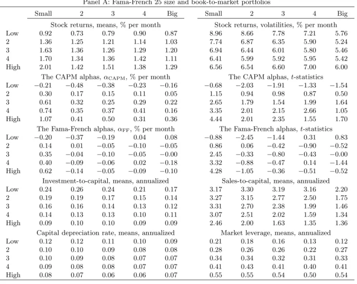
Table 1 reports descriptive statistics for all of our testing portfolios. We report means and volatil-ities of stock returns as well as the averages of key firm characteristics used in constructing the levered investment returns. These characteristics include the investment-to-assets ratio, the sales-to-capital ratio, the rate of capital depreciation, and market leverage.

Size and Book-to-Market Portfolios

Panel A of Table 1 reports the results for the Fama-French (1993) 25 size and book-to-market portfolios. The value premium (the average return of high book-to-market firms minus the average return of low book-to-market firms) is reliably positive in our sample, especially in small firms. The average return spread between the small-value and the small-growth portfolios is 1.10% per month (t-statistic = 4.96). In contrast, the average return spread between the big-value and big-growth portfolios is more than halved, 0.42% (t-statistic = 1.66). The CAPM and the Fama-French three-factor model have difficulty in explaining the average returns of the 25 portfolios. Ten out of the 25 CAPM alphas and four out of the 25 Fama-French alphas are statistically significant. In particular, the CAPM alpha of the small-stock value strategy (small-value minus small-growth) is 1.28% per month, and the Fama-French alpha is 0.82% per month. Both are highly significant.

The rest of Panel A in Table 1 reports in characteristic patterns that are suggestive of the

two-period example helps interpret the role of investment-to-capital, sales-to-capital, and the rate of depreciation. Panel A documents that growth firms have higher investment-to-capital ratios than value firms. The investment-to-capital spread between value and growth firms is 0.15 per annum in small firms, relative to 0.08 in big firms. In the context of equation (6), this investment pattern goes in the right direction for capturing the value premium, especially in small firms.

From Panel A of Table 1, growth firms have higher depreciation rates than value firms. The spread is 4% per annum in small firms, relative to 2% in big firms. The depreciation pattern also goes in the right direction for capturing the value premium, particularly in small firms. The reason is that, from equation (6), firms with higher depreciation rates earn lower expected returns than firms with lower depreciation rates, all else equal. This prediction on the relation between capital depreciation and average return is consistent with the theoretical work of Tuzel (2005). Using a two-sector model, Tuzel shows that firms with more structures earn higher average returns than firms with more equipment because structures depreciate more slowly than equipment.

In contrast, the sales-to-capital pattern goes in the wrong direction for capturing the value premium. From Panel A in Table 1, growth firms have a higher average sales-to-capital ratio than value firms. This evidence is consistent with Fama and French (1995), who show that growth firms have higher profitability than value firms. Further, the spread in sales-to-capital between value and growth in small firms is 0.71, which is smaller than that in big firms, 0.84. Our structural estimation jointly evaluates the quantitative importance of various expected-return determinants (see Section 6). Our results show that the investment and the depreciation channels dominate the sales-to-capital channel. As a result, the model is quantitatively successful for capturing the value anomaly. Panel A of Table 1 reports that value firms have higher market leverage ratios than growth firms, a well-known result in the empirical literature (e.g., Smith and Watts 1992). To sign the first-order effect, we differentiate the expected levered investment return with respect to leverage:

∂ Et[r I jt+1]−νjtEt[rjtB+1] 1−νjt ! /∂νjt= Et[rI jt+1]−Et[rBjt+1] (1−νjt)2 >0

The inequality follows because average stock returns (and therefore a linear combination of average stock and bond returns) are higher than average bond returns. The leverage spread between value and growth firms thus goes in the right direction for capturing the value premium.

Capital Investment Portfolios

From Panel B of Table 1, low investment-to-assets firms earn higher average returns than high investment-to-assets firms. The average return spread is 1.06% per month (t-statistic = 4.94). The CAPM alpha of the low-minus-high investment-to-assets strategy is 1.26% per month and the Fama-French (1993) alpha is 0.85%. Both are significant.

Because we form these portfolios by sorting on investment-to-assets, it is natural that the highest decile has a much higher investment-to-assets ratio, 0.36 per annum, than that of the lowest decile, 0.07. This large spread goes a long way in capturing the average return spread between the two ex-treme deciles. Besides investment-to-assets, the rate of depreciation and market leverage also go in the right direction for capturing the investment anomaly. In particular, the low investment-to-assets firms have an average depreciation rate of 6% per annum, which is lower than the depreciation rate of the high to-assets firms, 21%. Moreover, the market leverage of the low investment-to-assets firms is higher than that of the high investment-investment-to-assets firms: 0.48 versus 0.23. The sales-to-capital ratio goes in the wrong direction for capturing the average return spread, but this effect is quantitatively dominated by all the other channels, as our structural tests later show.

From Panel C of Table 1, the low-minus-high abnormal investment strategy `a la Titman, Wei, and Xie (2004) earns an average return of 0.59% per month, a CAPM alpha of 0.58%, and a Fama-French (1993) alpha of 0.52%. The t-statistics are 4.61, 3.95, and 3.88, respectively. The low abnormal investment decile has an investment-to-asset ratio of 9% per annum, which is only one half of that of the high abnormal investment decile, 18%. The leverage ratio of the low abnor-mal investment decile is somewhat higher than that of the high abnorabnor-mal investment decile: 0.40 versus 0.32, but the relation is not monotonic. The two other characteristics, sales-to-capital and depreciation rate, do not vary much across the ten abnormal investment portfolios.

Earnings Surprises Portfolios

From Panel D of Table 1, the high SUE decile outperforms the low SUE decile by on average 0.76% per month (t-statistic = 3.62). The CAPM and the Fama-French (1993) alphas for the high-minus-low SUE strategy are 0.79% and 1.01% per month, respectively, both of which are significant. The two-way sort on size and SUE in Panel E shows that the earnings anomaly is stronger in small firms. The average return spread between high and low SUE firms is 1.04% per month in small firms, 0.57% in median-size firms, and 0.14% in big firms. The respectivet-statistics are 8.21, 4.10,

and 1.00. The CAPM and the Fama-French (1993) alphas follow largely the same pattern.

The sales-to-capital pattern across SUE portfolios goes in the right direction for capturing post-earnings-announcement drift. From Panel D, sales-to-capital increases almost monotonically from 1.43 for the low SUE portfolio to 2.05 for the high SUE portfolio. From Panel E, high SUE firms also have higher sales-to-capital than low SUE firms in the two-way sort. The sales-to-capital spread in small firms is 0.68, which is higher than that in median-size firms, 0.47, which is in turn higher than that in big firms, 0.30. The ordering of the sales-to-capital spread across size terciles is intriguingly consistent with the ordering of the average-return spread.

In contrast, there is virtually no spread between high and low SUE firms in investment-to-assets and the rate of depreciation. This pattern is evident in both one-way and two-way sorts. However, low SUE firms have higher leverage than high SUE firms, a pattern that goes in the wrong direction for capturing the post-earnings-announcement drift. Our estimation later shows that the sales-to-capital channel quantitatively dominates the leverage channel. Nonetheless, the performance of our model in capturing the earnings anomaly is by no means perfect, probably because of leverage.

6

Structural Estimation

6.1 The Benchmark Model: Point Estimates and Overall Performance

We start with the benchmark specification, in which we lever the investment returns in the tests according to equation (29). The sample is monthly from January 1972 to December 2003.

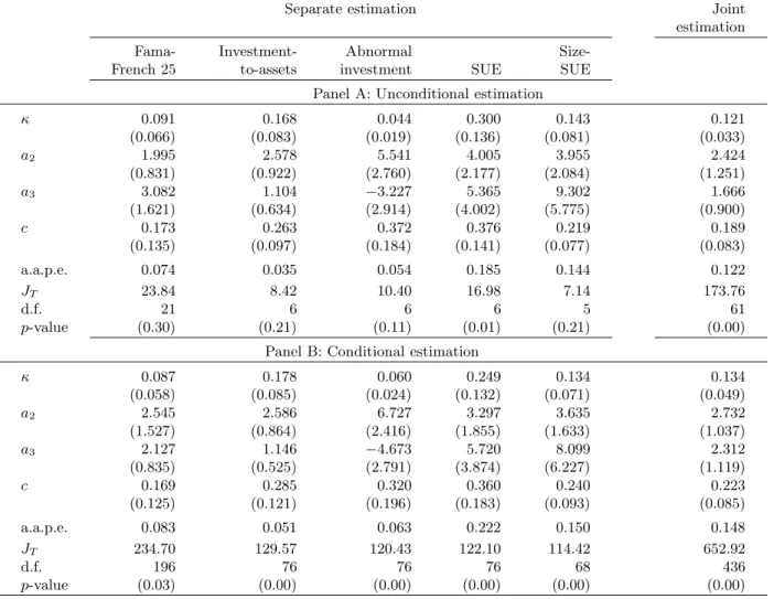
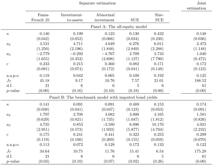
Table 2 reports parameter estimates and overall performance measures from both separate estimation and joint estimation. In the separate estimation, each set of portfolios constitutes its own moment conditions, and the parameter estimates differ across different portfolio sets. In the joint estimation, we pool all the testing portfolios together, and the parameter values are the same across all portfolios. We also report unconditional estimation, in which we use a vector of ones as the only instrument, and conditional estimation, in which we use our entire list of instrumental variables. In general, the parameter estimates across unconditional and conditional estimation are close.

From Table 2, the capital share,κ, is estimated from 0.09 and 0.30, and is often significant. The highest estimate occurs in the SUE-sorted portfolios. This result is reasonable because the model matches the SUE anomaly primarily by the average product of capital, and because higher estimates ofκproduce greater disperson in the fitted value of the average product across portfolios. From the positive and significant estimates of a2, the estimated adjustment-cost function is increasing and

convex. The estimates ofa3 indicate some evidence of higher-order nonlinearity in the adjustment-cost function. The estimated proportional operating adjustment-costs are all positive and often significant.

We also report two measures of overall model performance in Table 2. The first is the average absolute pricing errors that range only from 3.5 to 18.5 basis points per month for the unconditional estimation. The second is theJT overidentification tests. According to this metric, the benchmark model performs quite well when we use unconditional moment conditions to estimate separately the Fama-French (1993) 25 size and book-to-market portfolios, the nine size-SUE portfolios, the ten investment-to-assets portfolios, and the ten abnormal investment portfolios. The JT tests fail to reject the null hypothesis that the average levered investment returns equal the average stock returns. By adding more moment conditions, conditional estimation imposes more stringent tests on the model. The average absolute pricing errors generally increase, now ranging from 5.1 to 22.2 basis points per month. Correspondingly, with conditional estimation the JT tests produce rejections of the overidentifying restrictions for all sets of portfolios.

6.2 Alphas from the Benchmark Model

The average absolute pricing errors and the JT tests only give overall model performance. To provide a more complete picture, we report the alphas for all the testing portfolios. We define the alpha for one testing portfolio as its average stock return minus its average levered investment return constructed using estimated parameter values. The alpha is thus the pricing error for this portfolio.

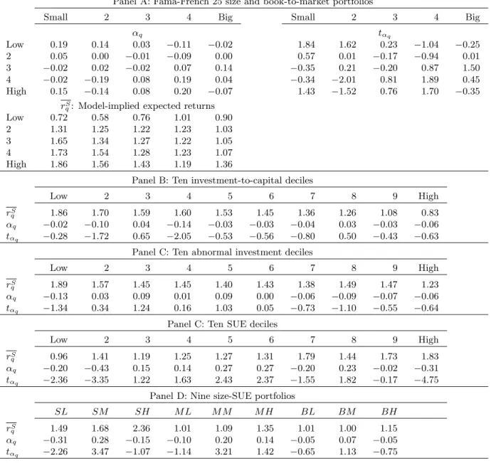
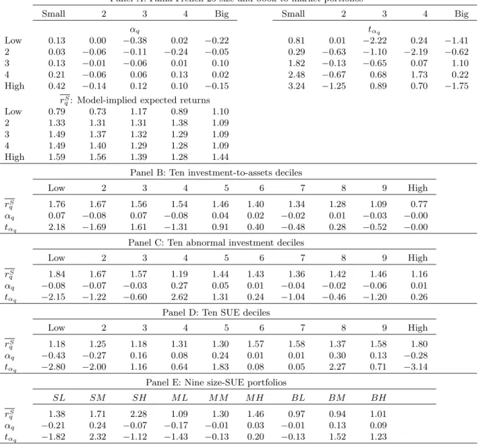
Unconditional and Separate Estimation

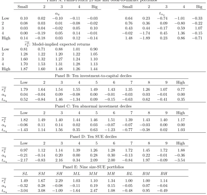
Table 3 reports the alphas from unconditional and separate estimation. From Panel A, the benchmark specification performs extremely well in capturing the average returns of the Fama-French (1993) 25 size and book-to-market portfolios. None of the alphas are significant. More importantly, the economic magnitudes of these alphas are small with the highest magnitude only 0.19% per month. The alphas of the small-growth and the small-value portfolios are only 0.10% and 0.14% per month (t-statistics = 0.64 and 1.48), respectively, suggesting that the alpha of the small-stock value strategy is only four basis points per month. This magnitude is negligible relative to the CAPM alpha of 1.28% per month or relative to the Fama-French (1993) alpha of 0.82% per month. The model thus captures the small-stock value anomaly that is notoriously difficult for traditional models (e.g., Fama and French 1996, Lettau and Ludvigson 2001, Campbell and Vuolteenaho 2004). From Panel B of Table 3, our model does particularly well in capturing the average returns of the

ten investment-to-assets deciles. None of the ten alphas are significant, and the highest magnitude of the alphas is only nine basis points per month. Panel C shows that our model also captures the average returns of ten abnormal investment deciles, even though we do not model overinvestment in our standard q-theoretic framework. None of the ten alphas are significant, and the highest magnitude of the alphas is only 0.14% per month. This evidence is comforting because one would hope that our investment-based asset pricing model could explain the investment-related anomalies. The model is only partially successful in matching the average returns of the ten SUE portfolios. From Panel D of Table 3, the low SUE decile earns an average levered investment return of 0.97% per month, and the high SUE decile earns 1.88%. This average return spread, 0.91% per month, in the model is quantitatively comparable to that in the data, 0.77% reported in Table 1. Moreover, the average returns from the model for deciles two and nine are 1.12% and 1.72% per month, which are close to their average stock returns of 0.98% and 1.71%, respectively. However, six out of ten alphas are individually significant, and the magnitudes of these alphas, which rise as high as 0.36% per month, are economically important.

Our model is more successful in generating the return patterns for the nine size-SUE portfolios. From Panel D of Table 3, only three of the nine alphas are significantly different from zero. The average return spread between the low and high SUE portfolios is about 0.80% per month in small firms, which is much higher than that in big firms, 0.14%. The model thus captures the stylized fact that the earnings anomaly is more pronounced in small firms.

Figure 2 provides a visual representation of the model performance by plotting the average levered investment returns of the testing portfolios against their average stock returns. With only a few exceptions, the observations are largely aligned with the 45-degree line.

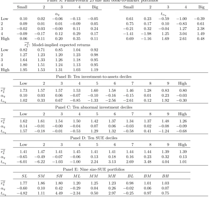
Unconditional and Joint Estimation

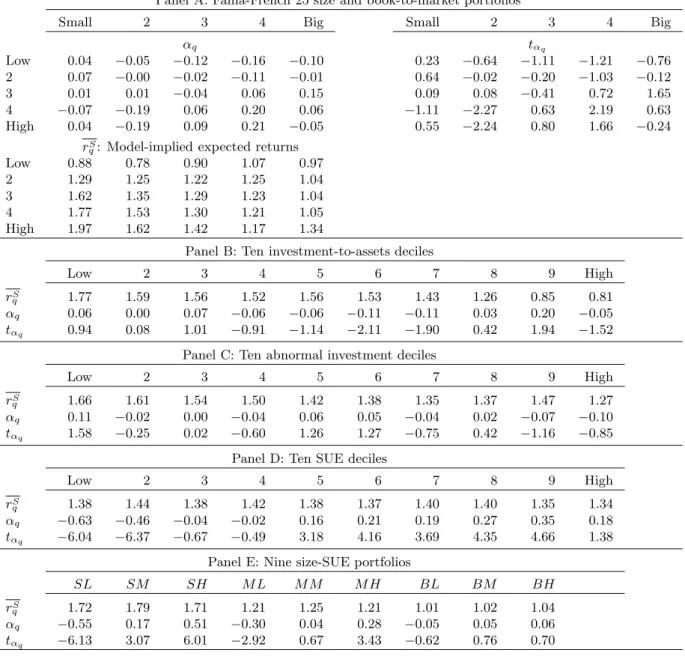
In joint estimation, because the model needs to match the average returns of all the testing portfo-lios, it is not surprising that the alphas are larger in magnitude than those in separate estimation. From Panel A of Table 4, three out of the Fama-French (1993) 25 portfolios now have significant alphas. More importantly, the model still does a good job in capturing the value premium in small firms. The two extreme book-to-market quintiles have an average return spread of 1.09% per month in small firms, relative to 0.37% in big firms.

joint estimation. From Panel B of Table 4, only one out of the ten investment-to-assets portfolios has a significant alpha. The sixth decile has an alpha of−0.11% per month (t-statistic = −2.11). From Panel C, none of the ten abnormal investment portfolios have significant alphas.

Unfortunately, the model loses its the ability to match the average returns of SUE portfolios in joint estimation, as shown in Panels D and E of Table 4. The model cannot generate the average-return spread of extreme SUE portfolios, and most portfolios have alphas that are individually significant. As a visual representation, the scatter plot in Panel D in Figure 3 shows a horizontal line for the ten SUE portfolios. The pattern for the nine size-SUE portfolios in Panel E is similar. However, the observations in Panels A to C for other testing portfolios are mostly aligned with the 45-degree line. The model performance is similar to that in Figure 2 for separate estimation.

Conditional Estimation

Table 5 reports the alphas for the testing portfolios in the benchmark specification with the con-ditional and separate estimation, and Table 6 reports the results with the concon-ditional and joint estimation. Because the use of instrumental variables produces many more moment conditions, the quantitative fit between the average stock returns and the average investment returns in the conditional estimation deteriorates slightly relative to that in the unconditional estimation. The magnitudes of the alphas are generally larger and more often significant. Nonetheless, the basic results of the alphas are quantitatively similar to those reported in Tables 3 and 4.

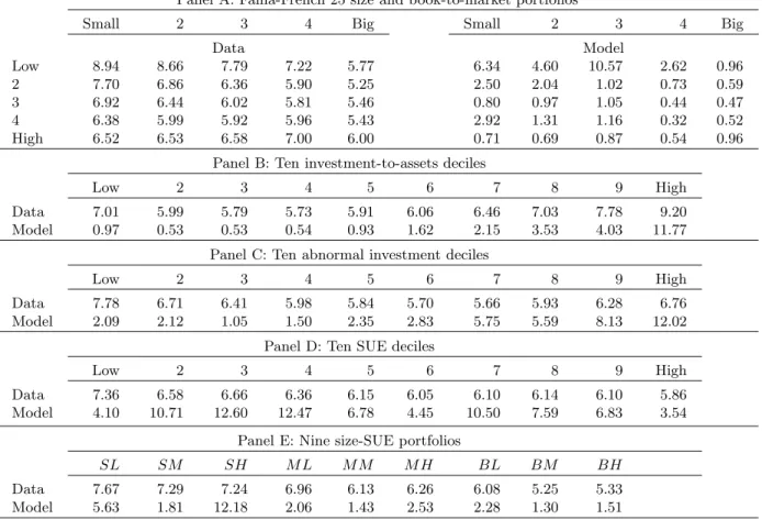
Volatilities

Table 7 reports the volatilities of portfolio stock returns and the volatilities of levered investment returns from the benchmark model.13 _{With a few exceptions, the model-implied volatilities are} generally lower than the volatilities observed in the data. This evidence is consistent with Cochrane (1991), who shows that aggregate investment returns are less volatile than aggregate stock returns. We reinforce his conclusion by showing that the same pattern also holds at the portfolio level.

6.3 Alternative Specifications

To evaluate the quantitative importance of different ingredients in our benchmark specification, we consider three perturbations: the all-equity model, the benchmark model with imputed bond yields,

13_{The model-implied volatilities reported in the table are based on the unconditional and separate estimation. The}

and the costly-external-equity model. We only report the unconditional and separate estimates. The results from other types of estimates are largely similar to those in the benchmark specification.

The All-Equity Model

Leverage is quantitatively important for capturing the small-stock value premium.

Panel A of Table 8 reports the parameter estimates and measures of overall performance for the all-equity model. The parameter estimates are quantitatively similar to those in the bench-mark model. In general, the average absolute pricing errors in the all-equity model are larger than those in the benchmark model. As a result, the all-equity model can be rejected in the case of the Fama-French (1993) 25 portfolios as well as in the case of the nine size-SUE portfolios. A notable exception is the ten SUE portfolios. The average pricing error decreases from 0.185% per month in the benchmark model to 0.109%, and the all-equity model cannot be rejected. In particular, the

p-value from the overidentification test is 18%.

Table 9 reports the alphas from the all-equity model. From Panel A, the model can still gen-erate the fact that the value premium is stronger in small firms than in big firms. However, the model leaves a small-stock value premium of 0.29% per month unexplained. In particular, the alpha for the small-value portfolio is 0.42% (t-statistic = 3.24). Comparing this evidence with Panel A of Table 3 therefore demonstrates the importance of leverage in capturing the small-stock value premium. All other aspects of Table 9 are quantitatively similar to the benchmark set of results.

The Benchmark Model with Imputed Bond Yields

The benchmark estimation assumes the Baa-rated bond yields for all testing portfolios. We now relax this assumption by imputing bond ratings using the methods of Blume, Lim, and MacKinlay (1998). With a few exceptions, the results are quantitatively similar to the benchmark results.

From Panel B of Table 8, the parameter estimates with imputed bond yields are close to those in the benchmark model. The average absolute pricing errors are somewhat higher than those from Table 2. In particular, the average pricing error across the Fama-French (1993) 25 portfolios increases from 0.074% per month in the benchmark case to 0.113% with imputed bond yields. As a result, the model can be rejected as the JT test has a p-value of 0.031. For all the other testing portfolios, the overall performance is similar to that of the benchmark specification.

From Table 10, the alphas for the benchmark model with imputed bond yields are quantitatively similar to those in the benchmark model. The model continues to do well in capturing the

small-stock value premium and in generating the average return spreads in ten investment-to-assets, ten abnormal investment portfolios, and ten SUE portfolios. Moreover, the model continues to predict that the SUE strategy works better in small firms than in big firms.

The Extended Model with Costly External Equity

The benchmark model assumes that firms can finance investment using external equity costlessly. In reality, issuing equity is costly, as evidenced by Smith (1977), Altinkilic and Hansen (2000), and Hennessy and Whited (2006). We thus extend the benchmark model to incorporate costly external equity. Because the extension is tedious, we leave the details to Appendix D. We only summarize the main insights from the extended model.

The extended model predicts that all else equal, firms that raise more equity should earn lower expected returns than firms that raise less external equity, consistent with the empirical literature on the new issues puzzle. We document that growth firms issue much more equity than value firms, especially in small firms. In particular, the new equity-to-capital spread between value and growth firms is 0.22 per annum in small firms, which is much higher than−0.02 in big firms. High investment-to-assets firms issue much more new equity than low investment-to-assets firms, 0.14 versus 0.01. However, the new equity-to-capital does not vary much across all other portfolios.

Untabulated results show that the extended model produces lower magnitudes of the pricing er-rors, especially for the conditional estimation, than the benchmark model. In particular, the model is not rejected in the conditional and separate estimation with the 25 size and book-to-market port-folios. Incorporating costly external equity also improves the model performance with the earnings portfolios. The unconditional and separate estimation yields an average absolute pricing error of 0.135% per month for the ten SUE portfolios and ap-value of 0.63 for theJT test. The average lev-ered investment returns for the two extreme SUE deciles are 0.82% and 1.52% per month. Further, the model predicts an average return spread of 1.38% per month between low- and high-SUE firms in small firms, relative to only 0.10% in big firms. TheJT test fails to reject the model with the nine size-SUE portfolios. All other results are quantitatively similar to those in the benchmark model.

7

Conclusion

The neoclassicalq-theory is a good start to understand the driving forces behind the cross section of returns. Under constant return to scale, stock returns equal levered investment returns, which

are tied directly to firm characteristics. This link provides a purely characteristics-based expected return model. We use a two-period example to show that the investment-return equation is qual-itatively consistent with the relations between average stock returns and book-to-market, capital investment, and earnings surprises. Using GMM, we also estimate the q-theoretic expected return model by minimizing the differences between average stock returns in the data and average levered investment returns in the model. Our model captures quite well the average returns of portfolios sorted on investment-to-assets, abnormal investment, and on size and book-to-market. Most impor-tant, the model accurately captures the small-stock value premium. The model is also partially suc-cessful in describing the post-earnings-announcement drift and its higher magnitude in small firms.

References

Abel, Andrew B. and Janice C. Eberly, 1994, A unified model of investment under uncertainty, American Economic Review 84 (1), 1369–1384.

Abel, Andrew B. and Janice C. Eberly, 2001, Investment and q with fixed costs: An empirical analysis, working paper, The Wharton School, University of Pennsylvania.

Altman, Edward I., 1968, Financial ratios, discriminant analysis, and the prediction of corporate bankruptcy,Journal of Finance 23, 589–609.

Altinkikic, Oya, and Robert S. Hansen, 2000, Are there economies of scale in underwriting fees? Evidence of rising external financing costs,Review of Financial Studies 13 (1), 191–218. Bansal, Ravi, Robert F. Dittmar, and Christian T. Lundblad, 2005, Consumption, dividends, and

the cross-section of equity returns,Journal of Finance 60 (4), 1639–1672.

Barberis, Nicholas, and Richard Thaler, 2003, A survey of behavioral finance, in George Constantinides, Milton Harris, and Rene Stulz, eds.: Handbook of the Economics of Finance (North-Holland, Amsterdam).

Balvers, Ronald J., and Dayong Huang, 2006, Productivity-based asset pricing: Theory and evidence, forthcoming,Journal of Financial Economics.

Belo, Frederico, 2006, A pure production-based asset pricing model, working paper, University of Minnesota.

Berk, Jonathan B, Richard C. Green, and Vasant Naik, 1999, Optimal investment, growth options, and security returns,Journal of Finance, 54, 1153–1607.

Bernanke, Ben S., and John Y. Campbell, 1988, Is there a corporate debt crisis? Brookings Papers on Economic Activity 1, 83–125.

Bernard, Victor L., 1993, Stock price reactions to earnings announcements: A summary of recent anomalous evidence and possible explanations, inAdvances in Behavioral Finance, edited by Richard H. Thaler, Russell Sage Foundation, New York.