Causal Discovery Beyond Conditional Independences

(1)

Causal Discovery

Beyond Conditional Independences

Dissertation

der Mathematisch-Naturwissenschaftlichen Fakult¨

at

der Eberhard Karls Universit¨

at T¨

ubingen

zur Erlangung des Grades eines

Doktors der Naturwissenschaften

(Dr. rer. nat.)

vorgelegt von

Eleni Sgouritsa

aus Athens/Greece

T¨

ubingen

2015

(2)

Gedruckt mit Genehmigung der Mathematisch-Naturwissenschaftlichen Fakultät der Eberhard Karls Universität Tübingen.

Tag der m¨undlichen Qualifikation: 29 October 2015

Dekan: Prof. Dr. Wolfgang Rosenstiel 1. Berichterstatter: Prof. Dr. Bernhard Sch¨olkopf 2. Berichterstatter: Prof. Dr. Felix Wichmann 3. Berichterstatter, falls zutreffend

(3)

(4)

(5)

Abstract

Knowledge about causal relationships is important because it enables the prediction of the effects of interventions that perturb the observed system. Specifically, predicting the results of interventions amounts to the ability of answering questions like the following: if one or more variables areforcedinto a particular state, how will the probability distribution of the other variables be affected? Causal relationships can be identified through randomized ex-periments. However, such experiments may often be unethical, too expensive or even impossible to perform. The development of methods to infer causal relationships from observational rather than experimental data constitutes therefore a fundamental research topic. In this thesis, we address the prob-lem of causal discovery, that is, recovering the underlying causal structure based on the joint probability distribution of the observed random variables. The causal graph cannot be determined by the observed joint distribution alone; additional causal assumptions, that link statistics to causality, are necessary. Under the Markov condition and the faithfulness assumption, conditional-independence-based methods estimate a set of Markov equiva-lent graphs. However, these methods cannot distinguish between two graphs belonging to the same Markov equivalence class. Alternative methods in-vestigate a different set of assumptions. A formal basis underlying these assumptions are functional models which model each variable as a function of its parents and some noise, with the noise variables assumed to be jointly independent. By restricting the function class, e.g., assuming additive noise, Markov equivalent graphs can become distinguishable. Variants of all afore-mentioned methods allow for the presence of confounders, which are unob-served common causes of two or more obunob-served variables.

(6)

6

In this thesis, we present complementary causal discovery methods employ-ing different kind of assumptions than the ones mentioned above. The first part of this work concerns causal discovery allowing for the presence of con-founders. We first propose a method that detects the existence and identifies a finite-range confounder of a set of observed dependent variables. It is based on a kernel method to identify finite mixtures of nonparametric product dis-tributions. Next, a property of a conditional distribution, called purity, is introduced which is used for excluding the presence of a low-range confounder of two observed variables that completely explains their dependence (we call low-range a variable whose range has “small” cardinality).

We further study the problem of causal discovery in the two-variable case, but now assuming no confounders. To this end, we exploit the principle of inde-pendence of causal mechanismsthat has been proposed in the literature. For the case of two variables, it states that, ifX →Y (X causes Y), then P(X) and P(Y|X) do not contain information about each other. Instead, P(Y) and P(X|Y) may contain information about each other. Consequently, esti-matingP(Y|X) fromP(X) should not be possible, while estimatingP(X|Y) based on P(Y) may be possible. We employ this asymmetry to propose a causal discovery method which decides upon the causal direction by compar-ing the accuracy of the estimations of P(Y|X) andP(X|Y).

Moreover, the principle of independence has implications for common ma-chine learning tasks such as semi-supervised learning, which are also dis-cussed in the current work.

Finally, the goal of the last part of this dissertation is to present empirical results on the performance of estimation procedures for causal discovery using Additive Noise Models (ANMs) in the two-variable case.

Experiments on synthetic and real data show that the algorithms proposed in this thesis often outperform state-of-the-art algorithms.

(7)

Acknowledgements

First and foremost, I would like to thank my advisors Dominik Janzing and Bernhard Sch¨olkopf for their great mentoring, continuous support and advice. They guided me during my studies in seeking for the right questions to ask but at the same time provided me with the flexibility to define my own research questions.

I would like to thank Dominik for his insightful guidance and constructive feedback. He was always available for my persistent questions which was essential to my progress. I have learned a lot from his perspective on what research is all about. His enthusiasm for pure research was contagious and motivational and he has contributed immensely in making my Ph.D. experi-ence inspirational and challenging.

I am also very grateful to Bernhard for giving me the opportunity to work in such a great and stimulating research environment. I would like to thank him for his inspiration, support and sharp discussions. He is undoubtedly one of the most prominent scientists in the field and I feel very lucky to have collaborated and learned from him. I would further like to sincerely thank the rest of my committee members for their time and help.

Special thanks to Jonas Peters for our collaboration during his time at MPI both as a Ph.D. student and later as a group leader of the causality group. It has always been a pleasure to discuss with him both scientifically and about life perspectives and I truly admire his drive and passion for research. I am also very thankful to my other co-authors Kun Zhang, Philipp Hen-ning, Samory Kpotufe, Joris Mooij and Oliver Stegle and to the rest of my colleagues from MPI for our fruitful scientific discussions. They created a friendly and cooperative working environment and an open atmosphere.

(8)

8

rina Rehbaum, our secretary, also contributed to this by always being very helpful, efficient and friendly.

I am also very fortunate to have exceptional friends from Athens, my home city. Sofia, Georgia, Manolis, Giannis, Foteini and others, although far, currently scattered around the world, have drastically contributed in making my life balanced and colorful. Moreover, a lot of fun moments of my time in T¨ubingen are due to my flatmate, Amalia, with whom I shared three fantastic years with endless discussions about life, politics and science.

Very special thanks to my parents and my wonderful sister for their love, constant support and encouragement during my studies. My mother was the first to introduce me to the beautiful world of mathematics and showed me the pleasure of learning and persistence in problem solving. Last but not least, my deep thanks to Giorgos for his long lasting support and patience during these years. His positive attitude, unconditional love and optimism kept me going.

(9)

Chapter 1 Introduction

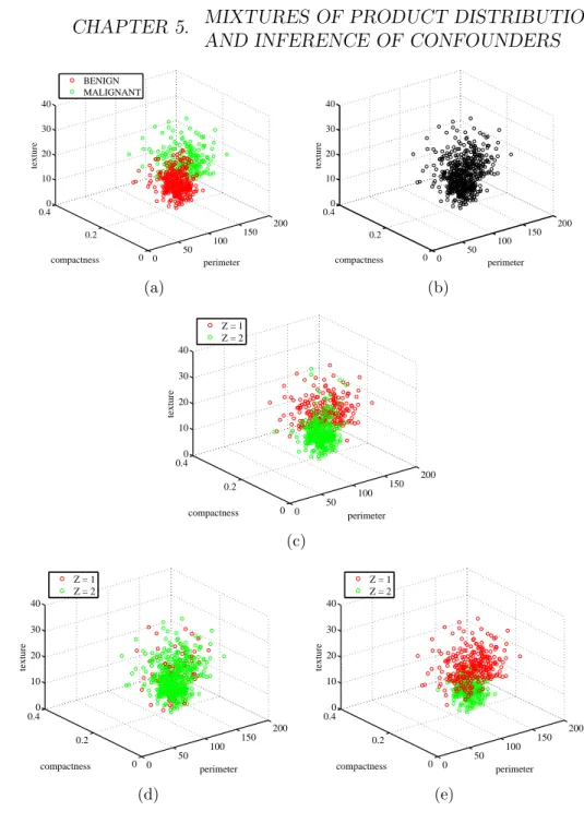
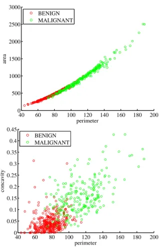
Machine learning is commonly concerned with prediction tasks [Bishop, 2006, Sch¨olkopf and Smola, 2002, Murphy, 2012], e.g., based on observations of the size and texture of a breast tumor, predict whether it is benign or ma-lignant (binary classification task). However, in many situations, the aim is to uncover the underlying causal mechanisms rather than just modeling the observed data. Cause-effect relationships tell us that a specific variable, say whether or not a person smokes, is not just statistically associated with a disease, but it is causal for the disease. Judea Pearl, ACM Turing award recipient in 2011, mentions in his book [Pearl, 2009]: “I now take causal rela-tionships to be the fundamental building blocks both of physical reality and of human understanding of that reality, and I regard probabilistic relation-ships as but the surface phenomena of the causal machinery that underlies and propels our understanding of the world.” and at a later part “...This puts into question the ruling paradigm of graphical models in statistics according to which conditional independence assumptions are the primary vehicle for expressing substantive knowledge. It seems that if conditional independence judgments are by-products of stored causal relationships, then tapping and representing those relationships directly would be a more natural and more reliable way of expressing what we know or believe about the world.” Besides being a more natural representation, a model built around causal rather than associational information offers the ability to predict the conse-quences of interventions. An intervention is the action of changing/disturbing

(14)

14 CHAPTER 1. INTRODUCTION smoking yellow teeth lung cancer

Figure 1.1: An explanation for the correlation between yellow teeth and lung cancer.

the “natural” probability distribution of some of the variables in a system, e.g., setting a given variable to some specified value. Knowledge about causal relationships enables the prediction of the effects of interventions, i.e., predic-tion of the system reacpredic-tion in hypothetical experiments that have not been performed.

Statistics alone is unable to aid in causal inference: for example, yellow stained teeth may be correlated with lung cancer, however this does not mean that yellow teeth is causal for lung cancer. That is, even though the color of the teeth can be a predictive feature for the presence of lung cancer, nevertheless, if an intervention whitens one’s teeth (e.g., by a visit to the dentist), this will not lead to the disappearance of the cancer. Instead, their statistical association could be explained by the presence of a third variable, say smoking, which is a common cause of both. This can be represented by the structure of Fig. 1.1, where arrows indicate causal relations.

One way of obtaining causal knowledge is through randomized trials. In our example, this would correspond to randomly staining the teeth of a part of the population and analyzing the difference in lung cancer between stained and not-stained populations. In the absence of difference, we would conclude that yellow teeth is not causal for lung cancer and seek alternative explanations for their correlation. However, randomized trials often cannot be performed in practice: they may be too expensive, unethical or even impossible. In this case, causal conclusions have to be drawn based solely on observational (and not interventional/experimental) data combined with appropriatecausal assumptions.

(15)

15 Under the Markov condition and the faithfulness assumption, independence-based methods [Spirtes et al., 2000, Pearl, 2009] estimate a set of directed acyclic graphs (DAGs), all entailing the same set of conditional indepen-dences, the so-called Markov equivalent graphs. However, these methods cannot distinguish between two graphs belonging to the same Markov equiv-alence class, e.g. X → Y and Y → X. Alternative methods investigate a different set of assumptions. A formal basis underlying these assumptions are functional models in which each variable is modeled as a function of its parents and some noise variable. The noise variables are assumed to be jointly independent. Restrictions on the function class, e.g., by assuming additive noise, can lead to distinguishing between graphs belonging to the same Markov equivalence class.

One major challenge of causal discovery is the possible presence of con-founders which are unobserved common causes of two or more observed vari-ables. The aforementioned methods, combined with assumptions about the existence of confounders, lead to different results concerning the identifiabil-ity of the structure.

This thesis investigates approaches, complementing existing ones, to infer the underlying causal DAG from observational data using various sets of assumptions. Chapter 5 proposes a method to infer the existence and identify a finite-range confounder of a set of observed dependent variables. It is based on a kernel method to identify finite mixtures of nonparametric product distributions. The number of mixture components is found by embedding the joint distribution into a reproducing kernel Hilbert space. The mixture components are then recovered by clustering according to an independence criterion. Chapter 6 is motivated by a problem in genetics. It builds on a property of a conditional distribution P(Y|X), which we call purity. Purity is used as a criterion to infer that the underlying causal structure isX →Y, as opposed to being a DAG containing a low-range latent variable Z in the path between X and Y such thatX ⊥⊥ Y|Z (X independent ofY given Z). Characterizing a conditional as pure is based on the location of the different conditionals{P(Y|X =x)}x in the simplex of probability distributions ofY.

Chapters 7 and 8 use the principle of independence of causal mechanisms which has been proposed in the literature. For the case of only two variables, it states that, if X → Y, the marginal distribution of the cause,P(X), and

(16)

16 CHAPTER 1. INTRODUCTION

the conditional of the effect given the cause, P(Y|X), are “independent”, in the sense that they do not contain information about each other. Instead, the distribution of the effect,P(Y), and the conditionalP(X|Y) may contain information about each other because each of them inherits properties from both P(X) and P(Y|X), hence introducing an asymmetry between cause and effect. This asymmetry has implications for common machine learning tasks such as semi-supervised learning (SSL), discussed in Chapter 7. One more implication of the principle of independence is that estimatingP(Y|X) from P(X) should not be possible. However, estimating P(X|Y) based on P(Y) may be possible. Chapter 8 focuses on the problem of causal discovery in the two-variable case, assuming no confounders. Employing the last im-plication we propose CURE, a causal discovery method which decides upon the causal direction by comparing the accuracy of the estimations ofP(Y|X) and P(X|Y) based on the corresponding marginals. To this end, we suggest a method for estimating a conditional based on samples from the marginal, which we call unsupervised inverse GP regression.

Finally, Chapter 9 presents empirical results on the behavior of estimation procedures for causal discovery using additive noise models, also concerning the two-variable case.

1.1 Thesis roadmap

In summary, this dissertation is organized as follows. Chapter 2 provides rel-evant background and basic concepts necessary throughout the thesis. Chap-ter 3 introduces the main problems tackled in this dissertation and ChapChap-ter 4 is devoted to a literature review of existing causal discovery methods and the assumptions they rely on. Chapters 5 includes a method for identifying a finite-range confounder of a set of observed variables, while Chapter 6 pro-poses a method for ruling out the existence of a low-range confounder of two observed variables that completely explains their dependence. Chapter 8 is concerned with causal discovery in the two-variable case but now assuming no confounders and is based on the principle of independence of causal mech-anisms. This principle has implications also for common machine learning tasks such as SSL, discussed in Chapter 7. Finally, Chapter 9 is concerned with the empirical behavior of estimation methods for ANMs.

(17)

1.1. THESIS ROADMAP 17 This dissertation covers material from the following publications:

• E. Sgouritsa, D. Janzing, J. Peters, and B. Sch¨olkopf. Identifying finite mixtures of nonparametric product distributions and causal inference of confounders. In Proceedings of the 29th International Conference on Uncertainty in Artificial Intelligence (UAI), 2013. (Chapter 5)

• D. Janzing, E. Sgouritsa, O. Stegle, J. Peters, and B. Sch¨olkopf. Detect-ing low-complexity unobserved causes. In Proceedings of the 27th In-ternational Conference on Uncertainty in Artificial Intelligence (UAI), 2011. (Chapter 6)

• B. Sch¨olkopf, D. Janzing, J. Peters, E. Sgouritsa, K. Zhang, and J. M. Mooij. On causal and anticausal learning. In Proceedings of the 29th International Conference on Machine Learning (ICML), 2012. (Chap-ter 7)

• E. Sgouritsa, D. Janzing, P. Hennig, and B. Sch¨olkopf. Inference of cause and effect with unsupervised inverse regression. InProceedings of the 18th International Conference on Artificial Intelligence and Statis-tics (AISTATS), 2015. (Chapter 8)

• S. Kpotufe, E. Sgouritsa, D. Janzing, and B. Sch¨olkopf. Consistency of causal inference under the additive noise model. In Proceedings of the 31st International Conference on Machine Learning (ICML), 2014. (Chapter 9)

(18)

(19)

Chapter 2 Background and basic concepts

In this chapter we first provide some background on graphs in Section 2.1 be-fore introducing Bayesian Networks (BNs) (Section 2.2) and causal Bayesian Networks (Section 2.3) to represent probabilistic and causal relationships, re-spectively. We further discuss an alternative representation using functional models in Section 2.4.

2.1 Graph notation

In the following, we shortly summarize definitions and notations on graphs. Basic graph definitions can be found, for example, in [Spirtes et al., 2000] and [Lauritzen, 1996]. A graph G consists of a set of vertices (or nodes) V ={1,2, . . . , d} and a set of edges (or links) E ⊆V2. If (a, b)∈E, then a is said to be a parentof b and b achild of a, denoted bya →b. The graph G1 = (V1, E1) is called a proper subgraph of G2 = (V2, E2) if V1 =V2 and

E1 ⊂E2. Theskeleton ofGis the undirected graph resulting from ignoring

all arrowheads in G. Moreover, a path is a sequence of distinct vertices v1, v2, . . . , vn such that (vi, vi+1)∈E or (vi+1, vi)∈E for alli= 1, . . . , n−1.

A directed path is a path v1, v2, . . . , vn such that (vi, vi+1) ∈ E for all

i = 1, . . . , n−1. An ancestor of a vertex a is any vertex b such that there is a directed path from b toa. Accordingly, adescendant ofa is any bsuch that there is a directed path from a tob. In a path v1, . . . , vn, vi is called a

(20)

20 CHAPTER 2. BACKGROUND AND BASIC CONCEPTS

colliderif (vi+1, vi)∈E and (vi−1, vi)∈E. A directed acyclic graph (DAG)

is a graph in which there is no directed path v1, v2, . . . , vn with v1 = vn. A

v-structure consists of two edges whose arrows point to the same vertex and whose tails are not connected by an edge. A topological ordering of a DAG is a sequence v1, v2, . . . , vn of its vertices such that for every edge

(a, b)∈E, vertex a comes before vertexb in the ordering.

A path between two vertices a and b is said to be unblocked (also called d-connected or open) conditioned on a set of vertices Z, with neither a nor b inZ, if and only if:

1. For every collider win the path, either w or a descendant of w is in Z 2. No non-collider in the path is in Z

A blocked path is a path that is not unblocked.

Definition 1 (d-separation) Two disjoint sets of vertices A and B are said to be d-separated given a set of vertices Z (also disjoint) if every path between any vertex in A and any vertex in B is blocked conditioned on Z.

2.2 Bayesian Networks

DAGs have been extensively used to represent a set of random variables and their conditional (in)dependences and came to be known as Bayesian Networks (BNs) [Pearl, 1988]. In a probabilistic graphical model (Bayesian Network), each node v ∈ V of the graph represents a random variable Xv

and the links express probabilistic relations between these variables. We denote random variables with capital letters and their corresponding values with lower case letters, e.g., X and x, respectively. Random vectors are denoted with bold face capital letters and their values with bold face lower case letters, e.g., X and x, respectively.

Considerd random variablesX:= (X1, X2, . . . , Xd)1 with rangesX1, . . . ,Xd,

respectively, and denote by P(X) their joint distribution. Unless stated

1_{We sometimes overload notation and use}_X_{to also denote the}_set_{_X

(21)

2.2. BAYESIAN NETWORKS 21 otherwise, assume P(X) has a density p(x) with respect to (w.r.t.) some product measure.

Definition 2 (Markov condition)The joint distribution P(X) is Markov w.r.t. the DAG G if the following equivalent statements hold:

• Markov factorization: p(x) factorizes as follows:

p(x1, x2, . . . , xd) = d

Y

j=1

p(xj|paj) (2.1)

where PAj is the set of parents of Xj in G.

• local Markov condition: every variable in G is conditionally indepen-dent of its non-descendants given its parents.

• global Markov condition:

A,B d-separated given Z in G⇒A⊥⊥B|Z

for all A,B,Z disjoint subsets of X.

Definition 3 (Bayesian Network) A Bayesian Network (BN) over X is a pair(G, P(X))such that the joint distributionP(X)is Markov with respect to the DAG G.

Two DAGs G1 and G2 are Markov equivalent (or alternatively belong to

the same Markov equivalence class) if the set of distributions that are Markov with respect to G1 coincides with the set of distributions that are Markov

w.r.t. G2. This is the case if the Markov condition entails the same set of

conditional independences. Verma and Pearl [1991] show that this happens if and only if the two graphs have the same skeleton and the same set of v-structures. For example, the DAGs X → Z → Y and X ← Z ← Y are Markov equivalent.

Definition 4 (minimality) A joint distribution P(X) satisfies minimality with respect to the DAG G if it is Markov w.r.t. G, but not to any proper subgraph of G.

(22)

Definition 5 (faithfulness) A joint distribution P(X) is faithful with re-spect to the DAG G if

A ⊥⊥B|Z⇒A,B d-separated given Z in G for all A,B,Z disjoint subsets of X.

In other words, faithfulness assumes that there are no conditional indepen-dences that are not entailed by the Markov condition.

2.3 Causal Bayesian Networks

Arrows in causal BNs do not merely represent probabilistic relations, as in BNs, but causal relations. In what follows, we formalize this concept. If an external intervention changes some aspect of the system under consideration, this may lead to a change in the joint distributionP(X). Specifically, an in-terventioncorresponds to a real world experiment that changes the “natural” probability distribution of a subset of the variables inX. We denote each such subset by XI := (Xi)i∈I, with rangeXI :=×i∈IXi,I ⊆ {1, . . . , d}. A special

kind of intervention is, for example, the so-calledhard orperfect intervention that forces a variableXto take on a certain valuex, symbolized asdo(X =x) [Pearl, 2009]. We first focus on the simplest case that|I|= 1, i.e., only one variable, say Xi, is intervened on. Then, P(X1, X2, . . . , Xd|do(Xi = xi)),

with i∈ {1, . . . , d}, denotes the joint distribution resulting after intervening on Xi ∈ X, setting Xi = xi. This is called an interventional distribution.

The latter is in contrast to the so-called observational distribution P(X), which is the joint distribution of X that we observe before conducting any experiment.

In the more general case, we intervene on more than one variable. Then, P(X1, X2, . . . , Xd|do(XI = xI)) denotes the interventional distribution,

re-sulting after intervening on XI, setting XI = xI := (xi)i∈I. Let Pdo(X) =

{P(X1, X2, . . . , Xd|do(XI = xI))}(I∈I)×(xI∈XI) denote the set of all possi-ble hard interventional distributions, with I standing for the power set of

(23)

2.3. CAUSAL BAYESIAN NETWORKS 23

Definition 6 (Causal Bayesian Network) The pair (G, P(X)) is called a causal Bayesian Network [Pearl, 2009], if, for every possible interventional distribution P(X1, X2, . . . , Xd|do(XI =xI))∈Pdo(X): p(x1, x2, . . . , xd|do(XI =xI)) = d Y j=1 j /∈I p(xj|paj) Y i∈I δXi,xi (2.2) where δXi,xi = 1 if Xi =xi 0 if Xi 6=xi

The right-hand side of Eq. (2.2) is called a truncated Markov factoriza-tion [Pearl, 2009], since it is equal to the original Markov factorization (Eq. (2.1)) but with some conditionals “truncated” (removed). According to Eq. (2.2), in a causal Bayesian Network, each interventional distribution (left-hand side) equals a truncated factorization, with the removed condi-tionals {P(Xi|PAi)}i being the ones of the intervened variables {Xi}i∈I.

It is worth noticing that _∅∈ I which corresponds to the special case of no intervention. Hence, the observational distribution P(X) can be considered a special interventional distribution (P(X)∈Pdo(X)) with no variable inter-vened on. In this case, Eq. (2.2) boils down to the (non truncated) Markov factorization of Eq. (2.1).

In the following, we often refer to the DAG Gof a causal Bayesian Network (G, P(X)) interchangeably as causal DAG, causal structure or causal graph. Furthermore, the conditional of each variable given its parents, P(Xj|PAj),

is often referred to as causal mechanism. We will henceforth assume that minimality is satisfied (see Definition 4).

The parents PAj of a variable Xj in a causal DAG can be thought of as its

direct causes w.r.t. the set of variables in X. In the special case of a causal DAG with only two variables in which X →Y,X is called the cause, Y the effect and we simply say that X causes Y.

For each intervention do(XI =xI), thecausal effect of XI on Y, denoted by

(24)

withXI andY disjoint subsets ofX[Pearl, 2009, Definition 3.2.1]. Consider

two random variablesX, Y ∈X. If there arex, x0 such thatP(Y|do(X =x)) is different from P(Y|do(X =x0)), then we say that X has a (total) causal effect on Y.

Interventions are not only limited to hard interventions that set variables to constants. A more general intervention corresponds to changing a causal mechanism P(Xj|PAj) to a new one, ˜P(Xj|PA˜ j). Then, the truncated

fac-torization in the right-hand side of Eq. (2.2) is replaced by the following factorization: d Y j=1 j /∈I p(xj|paj) Y i∈I ˜ p(xi|pa˜ i)

Usually the new set of parents ˜PAj is either empty or equals the old one,PAj.

In the former case, the type of intervention is often called stochastic [Korb et al., 2004], while in the lattermechanism change [Tian and Pearl, 2001] or parametric [Eberhardt and Scheines, 2007].

There are several advantages of causal Bayesian Networks over Bayesian Networks. The former are useful for predicting the effects of interventions, without having toactually perform the interventional experiment itself. Let (G, P(X)) be a causal Bayesian Network. By Definition 6, each interventional distribution in Pdo(X) can be computed just based on the causal DAG G and the observational distribution P(X), without actually performing any experiment. An interventional distribution can be obtained with only minor modifications in the Markov factorization of P(X), specifically, by just re-placing the conditionals of the intervened variables. A second advantage of causal BNs is that, roughly speaking, they are more natural and meaningful. For example, a machine learning scientist, not interested in causality, would still consider the graph of Fig. 1.1 a more natural way to encode beliefs about conditional independences than a graph in which the arrow between yellow teeth and smoking is reversed, even though both represent exactly the same conditional independences.

Note that there are cases where there is no causal BN over a set of variables. For example [Peters, 2012, Example 1.6], let X ← Z → Y be the DAG of a causal BN over the variables X, Y, Z. Then, there is no causal BN over

(25)

2.4. FUNCTIONAL MODELS 25 only X, Y since there is no DAG satisfying Definition 6 only for these two variables. On the other hand, ifX →Z →Y is the DAG of a causal BN over X, Y, Z, then there is a causal BN overX, Y with DAGX →Y. In contrast, there are (non causal) BNs over X, Y, with DAGs X → Y or Y → X, in both of the above scenarios, since P(X, Y) is Markov to both of these DAGs.

Proposition 1 (uniqueness) If there is a causal BN(G, P(X))overXand P(X) satisfies minimality w.r.t G, then G is unique in the sense that there is no other graph G0 such that (G0, P(X)) is a causal BN over X [Peters, 2012, Proposition 1.4].

Definition 7 (causal sufficiency) X1, X2, . . . , Xd is a causally sufficient

set of variables if there is a causal BN over them [Peters, 2012, Definition 1.9].

An alternative definition of causal sufficiency can be found in the literature,2

e.g., [Spirtes, 2010]: the random variables in X are causally sufficient if and only if there is no variable C /∈ X such that C is a direct cause of two or more variables in Xrelative to C∪X. If such a variableC exists, it is called a confounder, so causal sufficiency amounts to assuming that there are no confounders.

2.4 Functional models

An alternative way of expressing causal/probabilistic relationships is in the form of functional causal/probabilistic models [Pearl, 2009]. They consist of deterministic functional equations and probabilities are introduced through the assumption that certain variables (noise) in the equations are unobserved.

2_{This definition is slightly different from Definition 7. For an example consult the}

(26)

2.4.1 Functional probabilistic models

A functional probabilistic model (FPM) consists of a set ofd equations, one for each Xj ∈X:

Xj =fj(PAj, Nj), j = 1, . . . , d, (2.3)

wherePAj ⊆X, for all j, andN1, N2, . . . , Nd represent latent noise variables

which are assumed to be jointly independent: P(N) =

d

Q

j=1

P(Nj).

Drawing directed edges from each variable inPAjtoXj, for eachj, we obtain

a directed graph G corresponding to the FPM. This explains the common symbolPAj of this representation with the BN representation of Sections 2.2

and 2.3. In addition, G is required to be acyclic (DAG).

An FPM (for specific functions f1, . . . , fd, noise distributions P(N1), . . . ,

P(Nd), and parents sets PA1, . . . ,PAd) induces a unique joint distribution

over X: using a topological ordering3 _{of the DAG, each variable} _X

j can

be written as a function of the noise variables of the preceding variables. If the induced distribution of an FPM is identical to the joint distribution P(X) that we consider, we say that “the FPM induces/entails a distribution identical to P(X)” or, shortly, that “the FPM induces/entailsP(X)”. Pearl [2009, Theorem 1.4.1] shows that ifP(X) is induced by an FPM then it is Markov w.r.t. the DAGGof the FPM. Thus, (G, P(X)) is a Bayesian Net-work. Moreover, for every Bayesian Network (G, P(X)) there exists an FPM that induces a distribution identical to P(X) (see [Pearl, 2009, p. 31] and references therein). So, we can regard FPMs as an alternative to Bayesian Networks to encode joint distributions: the parent sets define the structure while the functions and noise distributions the parameters (conditional distri-butions). Note, however, that an FPM contains more information than a BN since many combinations of functions and noise distributions can correspond to the same conditional distributions.

An FPM refers to fixed functions, parent sets and noise distributions of the equations in (2.3), inducing a unique joint distribution. Varying parent

(27)

2.4. FUNCTIONAL MODELS 27 sets, functions and/or noise distributions results in different FPMs inducing various joint distributions.

Finally, it should be emphasized that FPMs are purely statistical models, as are Bayesian Networks, and not causal. We describe in the next section functional causal models (a.k.a. structural equation models) which are causal models, as are causal Bayesian Networks. A topological ordering of the DAG corresponding to an FPM does not necessarily correspond to a causal ordering. Instead, the FPM describes P(X) only through the fact that its induced distribution coincides with P(X). An FPM can be alternatively thought of as a set of regression models, one for each variable.

2.4.2 Functional causal models

Functional causal models (FCMs) (often referred to as Structural Equation Models (SEM)) [Pearl, 2009] are the causal counterpart of FPMs, same as causal Bayesian Networks as compared to Bayesian Networks. Specifically, similar to an FPM, a functional causal model consists of a set ofd equations, one for each Xj ∈X (Eq. 2.3).

The crucial difference is that a functional causal model M, just like a causal BN, represents the system under interventions [Pearl, 2009]: every interven-tional distribution P(X1, X2, . . . , Xd|do(XI =xI))∈Pdo(X) is equal to the distribution induced by the following set of equations:

Xj =fj(PAj, Nj), j /∈I

Xi =xi, i∈I

This set of equations is constructed from Mby replacing the equations cor-responding to the intervened variables with Xi =xi, i∈I, while leaving the

rest of equations intact. Thus, if Gis the (causal) DAG of an FCM inducing P(X), then (G, P(X)) is a causal Bayesian Network.

We finally note that functional causal models, as defined above, are called Markovian causal models by Pearl [2009, p. 30].

(28)

2.5 When the graph is known

If the causal graphGis known, for example from prior knowledge, then causal effects (see Section 2.3) can be computed. For example, the causal effect of a variableX on another variableY is given by the following formula [Pearl, 2009, Theorem 3.2.2] known as parent adjustment or adjustment for direct causes:4

p(y|do(Xi =xi)) =

X

pai

p(y|xi,pai)p(pai)

It is enough if the parents of the intervened variable are observed in this case. Yet the more challenging problem is to derive causal effects in situations where some members ofPAi are unobserved. A causal effect is called

identi-fiable if it can be computed from the observational (pre-intervention) distri-bution and the graph structure. Graphical tests exist for deciding whether causal effects are identifiable like the back- and front-door criteria [Pearl, 2009]. More generally, the calculus of interventions, the so-calleddo-calculus, was developed by Pearl to facilitate the identification of causal effects. It has been proven to be complete [Shpitser and Pearl, 2006, Huang and Valtorta, 2006], that is, all identifiable causal effects can be computed by an iterative application of its three rules. Moreover, graphical criteria exist [Tian and Shpitser, 2010, Huang and Valtorta, 2006] to find these causal effects. The literature is rich in what can be achieved in case that the causal graph G is known, but further details fall out of the scope of this thesis. This dissertation concerns, instead, scenarios in which Gis unknown and we seek to find it.

(29)

Chapter 3 Problem statement

The previous chapter motivated the need for causal models: based only on the causal DAG G and the observational distribution P(X), the effects of interventions can be predicted. However, the causal DAG is usually not available and needs to be learned from the observed data, supplemented with additional assumptions. In what follows, we state the general problems concerning (causal) structure learning.

Consider d variables X := (X1, X2, . . . , Xd) and denote by P(X) their joint

distribution.

Problem 1 (structure learning)Consider a Bayesian Network(G, P(X)) or a functional probabilistic model with DAG G that induces P(X). If G is unknown, can G (or properties of/features of/information about G) be recovered from P(X)? Under what conditions/additional assumptions? Clearly, without additional assumptions, G cannot be uniquely recovered fromP(X), since there are many DAGs to whichP(X) is Markov, e.g., to any fully connected acyclic graph. Imposing appropriate additional assumptions on the set of possible FPMs or BNs can lead to structure-identifiability, explained below:

Definition 8 (structure-identifiability) A set of BNs is called structure-identifiable if for any two Bayesian Networks (G1, P1(X)) and (G2, P2(X))

(30)

30 CHAPTER 3. PROBLEM STATEMENT

in this set:

P1(X) =P2(X)⇒G1 =G2 (3.1)

In other words, structure-identifiability means that the DAG can be uniquely recovered based on the joint distribution.1 _{The assumptions made often do}

not allow one to uniquely determine G but only a set of DAGs. We then have identifiability up to a class of DAGs. Definition 8 can also be adjusted to refer to FPMs apart from BNs: a set of FPMs is structure-identifiable if for any two FPMs with DAGsG1 and G2 inducing distributions P1(X) and

P2(X), respectively, (3.1) holds.

Problems 2, 3 and 4, that follow, describe variations of Problem 1 whenG is acausalgraph and/or whenlatentvariables are allowed. If the DAGG, that we seek for, is a causal DAG then structure learning is referred to ascausal discoveryor causal structure learning.

Problem 2 (causal structure learning)Consider a causal Bayesian Net-work(G, P(X))or a functional causal model with graph Gthat entailsP(X). IfGis unknown, canG(or properties of G) be recovered fromP(X)?2 _Under

what conditions/additional assumptions?

Let L := (L1, L2, . . . , Ll) be l unobserved random variables. Denote by

P(X,L) the joint distribution of (X,L).

Problem 3 (structure learning with latent variables) Consider a BN (G, P(X,L)) or a functional probabilistic model with DAG G that induces P(X,L). If G is unknown, can G (or properties of G) be recovered from P(X)? Under what conditions/additional assumptions?

1_{Structure-identifiability is often referred to, in related literature, simply as}

identifia-bility. In this thesis we use this term to discriminate it from parameter-identifiability (see Section 5.2) which means that the model parameters can be uniquely recovered from the joint distribution. Whenever the meaning is clear from the context, we also simply refer to an identifiable model without further specification.

(31)

31

Problem 4 (causal structure learning with latent variables) Consi-der a causal Bayesian Network(G, P(X,L))or a functional causal model with graph Gthat induces P(X,L). CanG (or properties ofG) be recovered from P(X)? Under what conditions/additional assumptions?

This thesis proposes methods to solve variations of Problems 2 and 4 by considering appropriate additional assumptions. For simplicity, sometimes we first present a method for usual structure learning (Problems 1 or 3) before attaching a causal meaning to it (Problems 2 or 4, respectively). In the former the additional assumptions considered can be viewed as statistical assumptions while in the latter as causal assumptions.

(32)

(33)

Chapter 4 Literature review

In this chapter, we review various methods for (causal) structure learning. The following approaches tackle the problems of Chapter 3 by considering additional assumptions that render G identifiable (often up to a class of DAGs) from the joint distribution. Section 4.1 deals with Problems 1 and 2, while Section 4.2 concerns Problems 3 and 4. Since there is a lot of related work on structure learning methods, this review is not exhaustive and mainly focuses on methods intended for causal structure learning.

4.1 Structure learning without latent

vari-ables

The literature is rich in methods for learning the structure of a Bayesian Network (Problem 1) or a causal Bayesian Network (Problem 2), assuming no latent variables. These can be divided based on the assumptions they make, e.g., faithfulness or additive noise, leading to different structure-identifiability results, e.g., identifiability up or within Markov equivalence classes.

(34)

34 CHAPTER 4. LITERATURE REVIEW

4.1.1 Independence-based methods

To solve Problems 1 and 2, conditional-independence-based methods [Spirtes et al., 2000, Pearl, 2009] (often referred to as constraint-based methods) assume that the observed joint distribution P(X) is not only Markov but also faithful relative to G (see Definition 5). This means that two disjoint subsets of variables A and B are conditionally independent given Z (also disjoint) if and only if A and B are d-separated given Z in G:

A,B d-separated given Z⇔A⊥⊥B|Z.

These methods are based on conditional independences between variables in

X: for two variables X, Y ∈ X, if there exists a subset Z of X\ {X, Y}

such that X ⊥⊥ Y|Z, then there is no edge between X and Y in G. This way the skeleton of G can be found. At a subsequent stage, a number of orientation rules is used to direct some of the edges. The output is a graph representing a set of Markov equivalent DAGs, all entailing the same set of conditional independences. Graphs within this Markov equivalence class cannot be distinguished without further assumptions. For example, if no conditional independences are observed, in the case of only two variables,

X= (X, Y), constraint-based methods output both X →Y and Y →X. Algorithms in this category include the IC [Pearl, 2009], the SGS [Spirtes et al., 2000] and the PC [Spirtes et al., 2000] algorithm. There are differ-ences between them including, but not limited to, the number of required conditional independence tests and the size of the conditioning sets. Condi-tional independence testing with large conditioning sets is a challenging task in practice.

4.1.2 Bayesian/score-based methods

Score-based methods, e.g., Cooper and Herskovits [1992], Heckerman et al. [1995], Geiger and Heckerman [1994], Heckerman [1995], Chickering [2002], have two basic components: a scoring metric and a search procedure. The metric computes a score for every candidate DAG, reflecting the goodness-of-fit of the structure to the data. In Bayesian methods, the score is pro-portional to the posterior probability of a structure given the data and any

(35)

4.1. STRUCTURE LEARNING WITHOUT LATENT VARIABLES 35 prior knowledge. The search procedure generates networks that are evalu-ated by the scoring metric. For discrete variables a multinomial likelihood can be used [Cooper and Herskovits, 1992, Heckerman et al., 1995], whereas for continuous variables a linear Gaussian model can be employed [Geiger and Heckerman, 1994]. DAGs that are Markov equivalent receive usually the same score, but there are some exceptions [Cooper and Herskovits, 1992]. Finally, there exist hybrid approaches that combine aspects of both constraint-based and score-constraint-based methods, e.g., Tsamardinos et al. [2006], Claassen and Heskes [2012].

4.1.3 Methods restricting the class of functional model

Unless supplemented with domain or expert knowledge, most of the previous structure learning methods cannot, in general, distinguish between DAGs belonging to the same Markov equivalence class (even if few score-based methods assign different scores to DAGs belonging to the same equivalence class, their motivation seems unclear). In order to be able to distinguish between Markov equivalent DAGs (based only on observational data), the approaches presented in this section use the functional model representation (Section 2.4) along with additional appropriate assumptions.

We first focus on Problem 1. Without further assumptions, P(X) could be induced by many DAGs. The idea of this group of methods is to restrict the functions of the FPM. Restricting the function class, restricts the set of distributions that can be induced.

One such restriction is realized using Additive Noise Models (ANMs) pro-posed by Hoyer et al. [2009] and Peters et al. [2014]. An ANM is an FPM in which the noise is additive, that is the set of equations in (2.3) become:

Xj =fj(PAj) +Nj, j = 1, . . . , d.

Hoyer et al. [2009] and Peters et al. [2014] prove structure-identifiability (see Definition 8) of ANMs, explained below for the simplest case of two variables,

(36)

Consider an ANM with DAG X →Y: X =NX

Y =f(X) +NY, X ⊥⊥NY

whose induced distribution isP(X, Y). Then, in the generic case (up to some exceptions like the case of linearf and GaussianX andNY), there is no ANM

with DAG Y → X inducing the same joint distribution P(X, Y). That is, there is no functiong and noise variableNX such that X =g(Y) +NX, with

Y ⊥⊥ NX. This means that, in the generic case, the DAG can be uniquely

recovered from the joint distribution, i.e., ANMs are structure-identifiable. We often simply say that ANMs are identifiable. The structure learning algorithm then reads: whenever there is an ANM with DAG in one direction (say,X →Y) inducing the joint distributionP(X, Y), but there is no ANM with DAG in the other direction (Y →X) inducingP(X, Y), then the DAG corresponding to the former direction is inferred (in this case X →Y). The generalization to more than two variables is described in Peters et al. [2014]. Previous work by Shimizu et al. [2006] proves identifiability of ANMs when restricted to linear functions and non-Gaussian input and noise distri-butions (Linear Non-Gaussian Acyclic Model (LiNGAM)). A generalization of ANMs are the Post-Nonlinear Models (PNL) [Zhang and Hyv¨arinen, 2009], whereY =h(f(X) +NY), withNY ⊥⊥X andh an invertible function, which

are also identifiable, except for some special cases.

The approaches of this category overcome some disadvantages of the previous methods: they allow inference of the DAG within the Markov equivalence class and do not need to assume faithfulness, but only minimality.

Causal counterpart We can use the method above to solve Problem 2 by considering FCMs instead of FPMs. Then, the inferred DAG is the causal DAG G of Problem 2. Janzing and Steudel [2010] justify why causal struc-ture learning using ANMs is reasonable. In particular, they show that if P(X, Y) can be induced by an ANM with DAG X → Y, then the causal DAG Y →X is unlikely because it would require a specific tuning between the hypothetical distribution of the causeP(Y) and the hypothetical causal mechanism P(X|Y) to generate a distribution that admits an additive noise model from X to Y.1 Furthermore, Mooij et al. [2014] present empirical

(37)

4.1. STRUCTURE LEARNING WITHOUT LATENT VARIABLES 37 results providing evidence that additive-noise methods are indeed able to distinguish cause from effect using only purely observational data.

4.1.4 Methods based on the principle of independence

of causal mechanisms

To solve Problem 2, other causal inference methods are based on the principle of independence of causal mechanisms [Janzing and Sch¨olkopf, 2010, Lemeire and Dirkx, 2006, Janzing et al., 2012, Daniusis et al., 2010, Sch¨olkopf et al., 2012] which we state below for the simplest case of a causal BN with only two observed variables, assuming no confounders:

Postulate 1 (independence of input and mechanism) If X → Y, the marginal distribution of the cause, P(X), and the conditional distribution of the effect given the cause, P(Y|X), are “independent” in the sense that P(Y|X) contains no information about P(X) and vice versa.

The (causal) conditionalP(Y|X) can be thought of as themechanism trans-forming causeX to effectY. Then, Postulate 1 is plausible if we are dealing with a mechanism of nature that does not care what (input P(X)) we feed into it. This independence can be violated in the backward direction: the distribution of the effect P(Y) and the conditional P(X|Y) may contain in-formation about each other because each of them inherits properties from bothP(X) and P(Y|X). This constitutes an asymmetry between cause and effect. While Postulate 1 is abstract, the aforementioned approaches provide formalizations by specifying what is meant by independence or information: Janzing and Sch¨olkopf [2010] postulate algorithmic independence ofP(Y|X) andP(X), i.e. zero algorithmic mutual information: I(P(X) :P(Y|X))= 0.+ This is equivalent to saying that the shortest description (in the sense of Kol-mogorov complexity) of P(X, Y) is given by separate descriptionsP(X) and P(Y|X). Since Kolmogorov complexity is uncomputable, practical imple-mentations must rely on other notions of (in)dependence or information. When causal relations are deterministic, with Y = f(X), P(Y|X) is com-pletely determined by f, so independence between P(X) and P(Y|X) boils

(38)

down to independence between P(X) and f. For deterministic non-linear relations, Janzing et al. [2012] and Daniusis et al. [2010] define independence through uncorrelatedness between logf0 and the density of P(X) w.r.t. the Lebesgue measure,2 _{both viewed as random variables on [0,}_{1] with uniform}

measure. This is reformulated in terms of information geometry as a certain orthogonality in information space. The corresponding Information Geo-metric Causal Inference (IGCI) method sometimes also works for sufficiently small noise. The performance of IGCI on both real-world and simulated data has also been thoroughly studied by Mooij et al. [2014].

Mooij et al. [2010] infer the causal direction by Bayesian model selection, defining non-parametric priors on the distribution of the cause and the condi-tional of the effect given the cause that favor distributions of low complexity. The motivation of their method stems also from Postulate 1.

4.2 Structure learning with latent variables

This section is mainly concerned with Problem 4: causal discovery with la-tent variables. Fast Causal Inference (FCI) [Spirtes et al., 2000] extends PC to causal discovery with latent variables. It assumes that the joint distribu-tionP(X,L) in Problem 4 is, apart from Markov, also faithful relative to G. Based on conditional independences among the observed variablesX, it out-puts a set of Markov equivalent maximal ancestral graphs (MAGs) [Richard-son and Spirtes, 2002]. MAGs are another type of graphs that are closed un-der marginalization (as opposed to DAGs), a useful property when it comes to latent variables. Claassen et al. [2013] propose FCI+, a more computa-tionally efficient version of FCI.

To distinguish between Markov equivalent graphs, other methods make more assumptions. Silva et al. [2006], apart from faithfulness, make the following assumptions:

• No variable in X is an ancestor of a variable inL.

(39)

4.2. STRUCTURE LEARNING WITH LATENT VARIABLES 39

• The joint distribution of Y := (X,L) is induced by a linear ANM:

Yj =αjPAj +Nj, j = 1, . . . , d+l.

They propose a framework that distinguishes among different causal graphs based on observable tetrad constraints [Silva et al., 2006]. Their contribution is two-fold: their method (1) finds disjoint subsets of the observed variables for which the members of each subset are d-separated by a latent common cause, and (2) finds features of the Markov equivalence class of the latent structure.

Shimizu et al. [2009] extend LiNGAM [Shimizu et al., 2006] for Problems 3 and 4, assuming thatP(X,L) is entailed by a linear ANM with non-Gaussian noise distributions. They further assume that P(X,L) is faithful to G to output all possible DAGs where each latent variable is a root node and has at least two children.

Finally, Janzing et al. [2009] extend ANMs [Hoyer et al., 2009] for Problems 3 and 4 but for the special case of two observed (X = (X, Y)) and at most one latent variable, i.e., l = 0 or l = 1, which (if it exists) is a confounder of X and Y. Specifically, their method distinguishes between the following DAGs: X → Y, Y → X or X ← Z → Y, with Z an unobserved latent variable (confounder).

(40)

(41)

Chapter 5 Identifying finite mixtures of

nonparametric product

distributions and causal

inference of confounders

5.1 Introduction

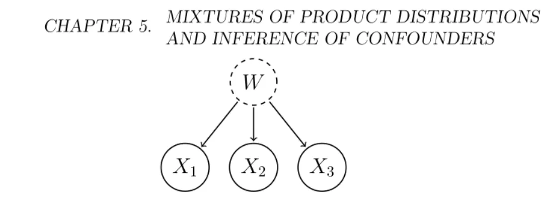
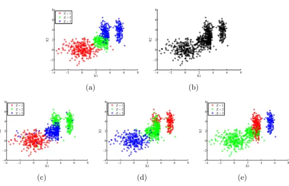
This chapter is concerned with Problems 3 and 4 (structure learning with latent variables). Specifically, the ultimate goal is to detect the existence and identify a finite-range hidden common cause, i.e., confounder, of a set of observed dependent variables. Consider, for example, that we observe three dependent variables X1, X2, X3. The goal is to be able to detect whether or

not their dependence is (only) due to a fourth latent variable, in practice of low range1_{, say} _W_{, that is a common cause of all of them (Fig. 5.1). In}

case that the DAG of Fig. 5.1 is inferred, we can also recover the full joint distribution P(X1, X2, X3, W), i.e., identify the confounder W.

To this end, we first propose a kernel method to identify finite mixtures of nonparametric product distributions. It is based on a Hilbert space

embed-1_{We call low range a random variable whose range has “small” cardinality.}

(42)

42 CHAPTER 5. MIXTURES OF PRODUCT DISTRIBUTIONS AND INFERENCE OF CONFOUNDERS

W

X

1

X

2

X

3

Figure 5.1: Motivating example of DAG to be inferred (the dotted circle represents an unobserved variable).

ding of the observed joint distribution. The rank of the constructed tensor is proven to be equal to the number of mixture components. We present an algorithm to recover the components by partitioning the data points into clusters such that the variables are jointly conditionally independent given the cluster label. We, then, show how this method can be used to identify finite-range confounders.

In Section 5.2, finite mixtures of product distributions are introduced. In Section 5.3, a method is proposed to determine the number of mixture com-ponents. Section 5.4 discusses established results on the identifiability of the component distributions. Section 5.5 presents an algorithm for determining the component distributions and Section 5.6 uses the findings of the previous sections for confounder detection and identification. Finally, the experiments are provided in Section 5.7.

5.2 Mixture of product distributions

Consider d ≥2 continuous observed random variables X1, X2, . . . , Xd with

ranges{Xj}1≤j≤dand assume that their joint distributionP(X1, . . . , Xd) has

a density with respect to the Lebesgue measure. Further, let Z be a finite-range (i.e., that takes on values from a finite set) latent variable2 _{with values}

in {z(1)_{, . . . , z}(m)_}_{. Only for Sections 5.3-5.5, let} _X

1, . . . , Xd be jointly

con-ditionally independent given Z, denoted by X1 ⊥⊥ X2 ⊥⊥ . . .⊥⊥ Xd|Z. This

(43)

5.3. IDENTIFYING THE NUMBER OF MIXTURE COMPONENTS 43 implies the following decomposition ofP(X1, . . . , Xd) into a finite mixture of

product distributions: P(X1, . . . , Xd) = m X i=1 P(z(i)) d Y j=1 P(Xj|z(i)) (5.1) where P(z(i)_{) =}_P_(Z ₌_z(i)₎₆_{= 0.}

By parameter identifiability of model (5.1), we refer to the question of when P(X1, . . . , Xd) uniquely determines the following parameters: (a) the

num-ber of mixture components m, and (b) the distribution of each component P(X1, . . . , Xd|z(i)) and the mixing weights P(z(i)) up to permutations of

z-values.3 In the next three sections, we focus on determining (a) and (b), when model (5.1) is identifiable. This can be further used to infer the existence of a latent variable confounding a set of observed variables and reconstruct this confounder (Section 5.6).

5.3 Identifying the number of mixture

com-ponents

Various methods have been proposed in the literature to select the number of mixture components in a mixture model (e.g., Feng and McCulloch [1996], B¨ohning and Seidel [2003], Rasmussen [2000], Iwata et al. [2013]). However, they impose different kind of assumptions than the conditional independence assumption of model (5.1), e.g., that the distributions of the components be-long to a certain parametric family. Assuming model (5.1), Kasahara and Shimotsu [2010] proposed a nonparametric method that requires discretiza-tion of the observed variables and provides only a lower bound on m. In the following, we present a method to determine m in (5.1) without making parametric assumptions on the component distributions.

3_{We interchangeably refer to}_m_{as the number of mixture components or as the number}

(44)

5.3.1 Hilbert space embedding of distributions

Our method relies on representingP(X1, . . . , Xd) as a vector in a reproducing

kernel Hilbert space (RKHS). We briefly introduce this framework. For a random variableX with rangeX, an RKHSH onX with kernelk is a space of functions f : X → _R with dot product h·,·i, satisfying the reproducing property [Sch¨olkopf and Smola, 2002]:

hf(·), k(x,·)i=f(x), and consequently,

hk(x,·), k(x0,·)i=k(x, x0)

The kernel thus defines a mapx 7→φ(x) :=k(x, .)∈ H satisfying k(x, x0) =

hφ(x), φ(x0)i, i.e., it corresponds to a dot product inH.

Let P denote the set of probability distributions on X, then we use the followingmean map [Smola et al., 2007] to define a Hilbert space embedding of P:

µ:P → H; P(X)7→_EX[φ(X)] (5.2)

We will henceforth assume this mapping to be injective, which is the case if k ischaracteristic [Fukumizu et al., 2008], as the widely used Gaussian RBF kernelk(x, x0) = exp(− kx−x0k2/(2σ2_)).

We use the above framework to define Hilbert space embeddings of distribu-tions of every single Xj. To this end, we define kernels kj for each Xj, with

feature maps xj 7→φj(xj) = k(xj, .)∈ Hj. We thus obtain an embedding µj

of the setPj into Hj as in (5.2).

We can apply the same framework to embed the set of joint distributions

P1,...,d on X1 ×. . .× Xd. We simply define a joint kernel k1,...,d by

k1,...,d((x1, . . . , xd),(x01, . . . , x 0 d)) = d Y j=1 kj(xj, x0j)

leading to a feature map into

H1,...,d := d

O

j=1

(45)

5.3. IDENTIFYING THE NUMBER OF MIXTURE COMPONENTS 45 with φ1,...,d(x1, . . . , xd) = d O j=1 φj(xj) where N

stands for the Hilbert space tensor product. We use the following mapping of the joint distribution:

µ1,...,d :P1,...,d → d O j=1 Hj P(X1, . . . , Xd)7→EX1,...,Xd[ d O j=1 φj(Xj)]

5.3.2 Identifying the number of components from the

rank of the joint embedding

By linearity of the mapsµ1,...,dandµj, the embedding of the joint distribution

decomposes into: UX1,...,Xd :=µ1,...,d(P(X1, . . . , Xd)) = m X i=1 P(z(i)) d O j=1 EXj[φj(Xj)|z (i)_] _(5.3)

Definition 9 (full rank conditional) Let A, B be two random variables with rangesA,B,respectively. The conditional probability distributionP(A|B) is called a full rank conditional if {P(A|b)}b∈B is a linearly independent set

of distributions.

Recalling that the rank of a tensor is the minimum number of rank 1 tensors needed to express it as a linear combination of them, we obtain:

Theorem 1 (number of mixture components) If P(X1, . . . , Xd) is

de-composable as in (5.1)andP(Xj|Z)is a full rank conditional for all1≤j ≤d,

(46)

Proof. From (5.3), the tensor rank ofUX1,...,Xd is at mostm. If the rank is m0 < m, there exists another decomposition of UX1,...,Xd (apart from (5.3)) asPm0

i=1

Nd

j=1vi,j, with non-zero vectorsvi,j ∈ Hj. Then, there exists a vector

w∈ H1, s.t. w⊥span{v1,1, . . . , vm0_,₁}andw6⊥span{(_E_X

1[φ1(X1)|z

(i)_])

1≤i≤m}.

The dual vector , wi defines a linear form H1 → R. By overloading

nota-tion, we consider it at the same time as a linear map H1 ⊗ · · · ⊗ Hd →

H2⊗ · · · ⊗ Hd,by extending it with the identity map onH2⊗ · · · ⊗ Hd. Then,

hPm0 i=1 Nd j=1vi,j, wi = Pm0 i=1hvi1, wi Nd

j=2vi,j = 0 but hUX1,...,Xd, wi 6= 0. So,

m=m0.

The assumption thatP(Xj|Z) is a full rank conditional, i.e.,{P(Xj|z(i))}i≤m

is a linearly independent set, is also used by Allman et al. [2009] (see Sec-tion 5.4). It does not preventP(Xj|z(q)) from being itself a mixture

distribu-tion, however, it implies that, for allj, q, P(Xj|z(q)) is not a linear

combina-tion of {P(Xj|z(r))}r6=q. Theorem 1 states that, under this assumption, the

number of mixture componentsmof (5.1) (or equivalently the number of val-ues ofZ) is identifiable and equal to the rank of UX1,...,Xd. A straightforward extension of Theorem 1 reads:

Lemma 1 (infinite Z) If Z takes values from an infinite set, then the ten-sor rank of UX1,...,Xd is infinite.

Although their connection to causal discovery may not be obvious yet, Theo-rem 1 and Lemma 1 are used later, in Section 5.6, for detecting the existence of a finite-range confounder.

5.3.3 Empirical estimation of the tensor rank from

fi-nite data

Given empirical data for everyXj,{x (1)

j , x

(2) j , . . . , x

(n)

j }, to estimate the rank

of UX1,...,Xd, we replace it with the empirical average

ˆ UX1,...,Xd := 1 n n X i=1 d O j=1 φj(x (i) j ), (5.4)

(47)

5.4. IDENTIFIABILITY OF COMPONENT DISTRIBUTIONS 47 which is known to converge to the expectation in Hilbert space norm [Smola et al., 2007].

The vector ˆUX1,...,Xd still lives in the infinite dimensional feature spaceH1,...,d, which is a space of functions X1 × · · · × Xd → R. To obtain a vector in a

finite dimensional space, we evaluate this function at the nd data points (x(q1)

1 , . . . , x (qd)

d ) with qj ∈ {1, . . . , n} (the d-tuple of superscripts (q1, . . . , qd)

runs over all elements of{1, . . . , n}d_{). Due to the reproducing kernel property,}

this is equivalent to computing the inner product with the images of these points under φ1,...,d: Vq1,...,qd := * ˆ UX1,...,Xd, d O j=1 φj(x (qj) j ) + = 1 n n X i=1 d Y j=1 kj(x (i) j , x (qj) j ) (5.5)

For d = 2, V is a matrix, so one can easily find low rank approximations via truncated Singular Value Decomposition (SVD) by dropping low SVs. For d >2, finding a low-rank approximation of a tensor is an ill-posed prob-lem [De Silva and Lim, 2008]. By grouping the variables into two sets, say X1, . . . , Xs and Xs+1, . . . , Xd without loss of generality, we can formally

ob-tain thed= 2 case with two vector-valued variables. This amounts to reduc-ing V in (5.5) to ann×nmatrix by settingq1 =· · ·=qsandqs+1 =· · ·=qd.

In theory, we expect the rank to be the same for all possible groupings. In practice, we report the rank estimation of the majority of all groupings. The computational complexity of this step is O(2d−1n3).

5.4 Identifiability of component distributions

Once we have determined the number of mixture components m of model (5.1), we proceed to step (b) (see Section 5.2) of recovering the distribution of each componentP(X1, . . . , Xd|z(i)) and the mixing weightsP(z(i)). In the

following, we describe results from the literature on when these parameters are identifiable, for knownm. Hall and Zhou [2003] proved that whenm= 2, identifiability of parameters always holds ind≥3 dimensions. Ford= 2 and m = 2 the parameters are generally not identifiable: there is a two-parameter continuum of solutions. Allman et al. [2009] established identifiability of the

(48)

parameters whenever d ≥ 3 and for all m under weak conditions4_{, using a}

theorem of Kruskal [1977]. Finally, Kasahara and Shimotsu [2010] provided complementary identifiability results for d ≥ 3 under different conditions with a constructive proof.

5.5 Identifying component distributions

Theorem 1 states that the number of mixture components m of model (5.1) can be identified with the rank of the Hilbert space embedding of P(X1, . . . , Xd). Further, Section 5.4 presented existing results concerning

the identifiability of the component distributions{P(X1, . . . , Xd|z(i))}1≤i≤m.

In this section, we propose an algorithm that identifies the mixture compo-nents. Specifically, consider n data points drawn from P(X1, . . . , Xd), with

P(X1, . . . , Xd) belonging to an identifiable model (5.1). Further, let m be

known (it can be estimated as described in Section 5.3.3). Our goal is to cluster the n data points using m labels in such a way that the distribution of points with labeliis close to theunobserved empirical distribution of every mixture component, Pn(X1, . . . , Xd|z(i)). In what follows, we often refer to

the number of mixture componentsm as the number of clusters.

5.5.1 Existing methods

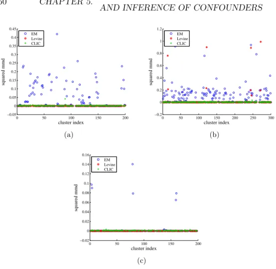
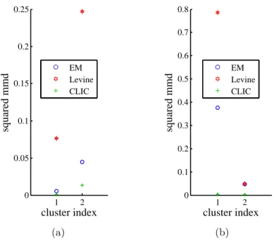
Probabilistic mixture models or other clustering methods can be used to iden-tify the mixture components (clusters) (e.g., von Luxburg [2007], B¨ohning and Seidel [2003], Rasmussen [2000], Iwata et al. [2013]). However, they impose different kind of assumptions than the conditional independence as-sumption of model (5.1) (e.g., Gaussian mixture model). Assuming model (5.1), Levine et al. [2011] proposed an Expectation-Maximization (EM) algo-rithm for nonparametric estimation of the parameters in (5.1), given thatm is known. Their algorithm uses a kernel as smoothing operator. They choose a common kernel bandwidth for all the components because otherwise their iterative algorithm is not guaranteed not to increase from one iteration to

4_{The same assumption used in Theorem 1, namely that}_P₍_X

j|Z) is a full rank

(49)

5.5. IDENTIFYING COMPONENT DISTRIBUTIONS 49 another. As stated also by Chauveau et al. [2010], the fact that they do not use an adaptive bandwidth [Benaglia et al., 2011] can be problematic especially when the distributions of the components differ significantly.

5.5.2 Proposed method: clustering with independence

criterion (CLIC)

The proposed method, CLIC (CLustering with Independence Criterion), as-signs each of the n observations to one of the m mixture components (clus-ters). We do not claim that each single data point is assigned correctly (especially when the clusters are overlapping). Instead, we aim to yield the variables jointly conditionally independent given the cluster (label) in order to recover the mixture components according to model (5.1).

To measure conditional independence of X1, . . . , Xd given the cluster we use

the Hilbert Schmidt Independence Criterion (HSIC) [Gretton et al., 2008]. It measures the Hilbert space distance between the kernel embeddings of the joint distribution of two (possibly multivariate) random variables and the product of their marginal distributions. Ifd >2, we test for mutual indepen-dence. For that, we perform multiple tests, namely: X1 against (X2, . . . , Xd),

then X2 against (X3, . . . , Xd) etc. and use Bonferroni correction. For each

cluster, we consider as test statistic the HSIC from the test that leads to the smallest p-value (“highest” dependence).

We regard the negative sum of the logarithms of all p-values (each one cor-responding to one cluster) under the null hypothesis of independence as our objective function. The proposed algorithm is iterative. We first randomly assign every data point to one mixture component. In every iteration we perform a greedy search: we randomly divide the data into disjoint sets of c points. Then, we select one of these sets and consider all possible assign-ments of the set’s points to the m clusters (mc possible assignments). The assignment that optimizes the objective function is accepted and the points of the set are assigned to their new clusters (which may coincide with the old ones). We, eventually, repeat the same procedure for all disjoint sets and this constitutes one iteration of our algorithm. After every iteration we test for conditional independence given the cluster. The algorithm stops after an iteration when any of the following happens: we observe independence in

Causal Discovery Beyond Conditional Independences