Large-scale data mining analytics based on MapReduce

Institute of Parallel and Distributed Systems

Applications of Parallel and Distributed

Systems

University of Stuttgart

Universitätsstraße 38

D - 70569 Stuttgart

Masterarbeit Nr. 3699

Large-scale Data Mining Analytics

Based on MapReduce

Sunny Ranjan

Studiengang:

Infotech

Prüfer:

PD Dr. Holger Schwarz

Betreuer:

PD Dr. Holger Schwarz

Begonnen am:

12.05.2014

Beendet am:

16.12.2014

CR-Classifikation:

H.2.8, H.3.4, D.4.3, D.4.7




!

!

aa

Anwendungssoftware

ss

Table of contents

Abstract

6

1. Introduction

7

1.1 Background Of The Problem 7

1.2 Purpose Of Work 9

1.3 Structure Of Work 12

2. Data Mining Concepts

13

2.1 Motivation Behind Data Mining 13

2.2 Definition Of Data Mining 14

2.3 Data Mining Process 15

2.4 Data Mining Methods And Its Categories 16

3. MapReduce Concepts

21

3.1 MapReduce Paradigm 21

3.2 Pre-Requisites 21

3.3 Architecture And Programming Model 22

4. Hadoop

24

4.1 HDFS - Hadoop Distributed File System 24

4.1.1 Design of HDFS 25

4.2 MapReduce Framework 26

4.2.1 Map 27

4.2.2 Reduce 28

4.3 Hadoop MapReduce 1.0 (MRv1) 28

4.4 Hadoop MapReduce 1.0 (MRv1) or YARN 30


4.5 Why YARN? 32


4.6 Conclusion 33

5. Apache Spark

34

5.1 Basics Of Spark 34


5.2. Overview Of Spark In Cluster Mode 37

5.3 Spark On YARN 38


5.4 Task Scheduling Process In Spark 40


5.5 Apache Spark’s Machine Learning Library (MLlib) 41


5.6 Decision Tree Learning Algorithms In Spark’s MLlib 41


6. Discussion Of Existing Approaches To Large Scale Data Mining

44




6.1. Existing MapReduce Based Data Mining Scientific Works 45

6.1.1 MapReduce Naive Bayes Classifier 45

6.1.2 MapReduce K-Means Clustering 47

6.1.3 MapReduce K-Medoids Clustering 48

6.1.4 MapReduce Co-Clustering 48

6.1.5 MapReduce Apriori Association Rule Discovery 49

6.1.6 MapReduce ID3 Decision Tree 50

6.1.7 MapReduce C4.5 Decision Tree 51

6.1.8 MapReduce Decision Tree Ensembles (PLANET) 53

6.2 MapReduce Based Data Mining Tools 55

6.2.1 Apache Mahout 55

6.2.2 WEKA 57

6.3 Conclusion 58

7. Experimental Set-Up

59

7.1 Data Preparation 63


8. Experimental Results and Evaluation

69

8.1 Initial Experiments 70


8.2. Experiment 1 With Alpha Data (Binary Classification) 70


8.3 Experiment 2 With Blog Data (Regression) 74

8.4 Experiment 3 With YearPrediction Data (Regression) 77


8.5 Experiment 4 With Mnist Data (Multi-Class Classification) 82


8.6 Conclusion 86

9. Conclusion Of This Work

89

References

90




List Of Figures

97




John Naisbett:

“We are drowning in data but starving for knowledge.”

Abstract

In this work, we search for possible approaches to large-scale data mining analytics. We perform an exploration about the existing MapReduce and other MapReduce-like frameworks for distributed data processing and the distributed file systems for distributed data storage. We study in detail about Hadoop Distributed File System (HDFS) and Hadoop MapReduce software framework. We analyse the benefits of newer version of Hadoop software framework which provides better scalability solution by segregating the cluster resource management task from MapReduce framework. This version is called YARN and is very flexible in supporting various kinds of distributed data processing other than batch-mode processing of MapReduce.

We also looked into various implementations of data mining algorithms based on MapReduce to derive a comprehensive concept about developing such algorithms. We also looked for various tools that provided MapRedcue based scalable data mining algorithms. We could only find Mahout as a tool specially based on Hadoop MapReduce. But the tool developer team decided to stop using Hadoop MapReduce and to use instead Apache Spark as the underlying execution engine. WEKA also has a very small subset of data mining algorithms implemented using MapReduce which is not properly maintained and supported by the developer team. Subsequently, we found out that Apache Spark, apart from providing an optimised and a faster execution engine for distributed processing also provided an accompanying library for machine learning algorithms. This library is called Machine Learning library (MLlib). Apache Spark claimed that it is much faster than Hadoop MapReduce as it exploits the advantages of in-memory computations which is particularly more beneficial for iterative workloads in case of data mining. Spark is designed to work on variety of clusters: YARN being one of them. It is designed to process the Hadoop data. We selected to perform a particular data mining task: decision tree learning based classification and regression data mining. We stored properly labelled training data for predictive mining tasks in HDFS. We set up a YARN cluster and run Spark’s MLlib applications on this cluster. These applications use the cluster managing capabilities of YARN and the distributed execution framework of Spark core services.

We performed several experiments to measure the performance gains, speed-up and scale-up of implementations of decision tree learning algorithms in Spark’s MLlib. We found out much better than expected results for our experiments. We achieved a much higher than ideal speed-up when we increased the number of nodes. The scale-up is also very excellent. There is a significant decrease in run-time for training decision tree models by increasing the number of nodes. This demonstrates that Spark’s MLlib decision tree learning algorithms for classification and regression analysis are highly scalable. 


1.

Introduction

We started this work with the objective of performing large-scale data mining analytics using MapReduce. With MapReduce, we mean a distributed data-processing model which has become popular for processing extremely large-scale data. We went on for an extensive search of implementations and tools of data mining algorithms which provided

large-scale data mining based on Hadoop MapReduce. We narrowed our search for a

specific data mining task: decision tree model learning based classification and regression data mining. We found out during our extensive search process that there are rather very few implementations of data mining algorithms based on Hadoop MapReduce. We found only two tools that supported some data mining algorithms based on original MapReduce. But we discovered that both of those tools have discontinued their support for original Hadoop MapReduce. The respective teams responsible for both the tools decided to completely retool their scalable data mining algorithms by using Apache Spark. This is how we came across Apache Spark.

Apache Spark is a MapReduce-like distributed data processing model that uses Hadoop data and Hadoop cluster but uses a much more optimised execution engine than the original Hadoop MapReduce [5a]. Their execution engine is optimised for different kinds of workloads as opposed to strict batch-mode processing of original MapReduce. Apache Spark not only provided an efficient execution that exploited the advantage of in-memory computations but also provided in-built low-level data structures and high-level libraries

(programming constructs) for data mining algorithms. This library is called Machine

Learning library, abbreviated as MLlib, which contains some high level APIs for performing a wide variety of data mining tasks. We also found out that it contained the implementations for decision tree learning based classification and regression analysis.

We go on to analyse the performance of those algorithms implemented in MLlib. We run programs using Apache Spark’ MLlib algorithms on a Hadoop YARN cluster which acts as a cluster manager and a Hadoop distributed files system for data storage. We use Apache Spark’s MLlib algorithms to build a decision tree of a fixed depth by using three different kinds of data mining tasks: binary classification, multi-class classification and regression. We perform numerous experiments with real-world data of varying sizes and various number of nodes to measure the performance gain, scale-up and speed-up. We also determine the impact of data characteristics and other factors on the computation time. We also elucidate the limitations and bottlenecks of building distributed scalable decision trees using this execution environment. We finally analyse the effectiveness of this distributed data-processing model and framework for mining large-scale data. We aim to find out if this library successfully serves our purpose for large-scale data mining.

1.1

Background Of The Problem

There is no dearth of data mining algorithms and tools for processing small datasets which can easily fit into a single machine (see a list of them in [1]). In order to mine large datasets, one of the current workarounds is to first sample the huge amounts of data into a smaller

dataset and then feed the resulting smaller dataset into the existing data mining algorithms and tools. This obviously does not alleviate the problem of storing such large-scale data and in addition to that, there are no such sampling algorithms which can guarantee to give always good sampling quality for any kind of data. As a result, this particular approach is not proven to output accurate data models. Therefore, large-scale data mining and analytics is still a much researched topic in Information Technology sector. Large-scale data mining and analytics is a term which usually refers to processing and analysis of “datasets with sizes which is beyond the capability of commonly used software tools to capture, curate, manage and process the data within a tolerable [and acceptable] elapsed time” [2]. The sudden explosion of data has driven the needs for more scalable and faster data mining and analytics methods. The conventional or legacy data mining algorithms, broadly classified into association-rule discovery, classification, regression and clustering suffer from the problems of memory and processing power limitations of the single machine they are running on.

So, how can we do large-scale data mining? MapReduce framework, first developed by Google, is the golden standard for general large-scale data processing and is slowly emerging as an important paradigm in data mining and analytics. MapReduce [3] is a simple programming model for expressing distributed computations on massive amounts of data and also an execution framework for large-scale data processing on clusters built from low-end commodity servers. With MapReduce, queries are split and distributed across parallel nodes and processed in parallel (the map step). The results are then collected from various map outputs and merged (the reduce step). The huge success of MapReduce has led to increasing implementations of data mining algorithms based on this framework. The high throughput and the performance of Google MapReduce subsequently led to the

open-source MapReduce implementation by Apache Software Foundation which is known as

Hadoop [4]. Although MapReduce is very simple because of its high-level abstraction and simplistic programming model, its application to the data mining algorithms remains poorly understood. The conversion of legacy algorithms to MapReduce is, henceforth, a non-trivial process. The process of designing MapReduce data mining algorithms requires identifying the parts of the legacy algorithms which have independence with respect to data and can be parallelized. Moreover, it also obligates the algorithm designers to develop a proper understanding of the MapReduce architecture.

MapReduce has continuously evolved over years in an effort to yield ever-increasing throughput and performance. These optimised MapReduce frameworks are called MapReduce-like frameworks. But in essence, they are MapReduce because they distribute the computations using map function and combine the results in reduce function. Nowadays, there are numerous implementations of MapReduce and that’s why it is a very broad term that encompasses the original MapReduce and the optimised versions. The optimised versions of MapReduce rather than the pure Hadoop MapReduce was found to be interesting for our work because a lot of work has been already done using old MapReduce systems and they clearly point out the drawback of strict batch-processing model for heavily iterative algorithms like data-mining algorithms. Moreover, hadoop MapReduce clusters are hardcoded to perform only MapReduce batch workloads and cannot support other workloads. This was seen as a wastage of valuable computational

resources. As a consequence, it is interesting for us to analyse a computational framework which is basically tailored for our purpose. Apache Spark [5] is a relatively new distributed processing engine for large-scale data which promises a much faster performance as compared to Hadoop MapReduce in general. This is made possible by persisting as much data in memory as possible and performing in-memory MapReduce based distributed computation. This saves the time for multi-stage applications as they do not need to perform the expensive disk read operations in every stages. This concept of data caching is particularly useful for iterative workflows where computations are done on nearly same datasets in every iterations [5a]. Apache spark provides a rich set of tools that take advantage of its optimised core execution engine. They are customised for special workflows like streaming, graph-processing, iterative processing, etc in order to optimise the MapReduce for a particular kind of data processing. One of such libraries is called Machine Learning library (MLlib) which optimises the MapReduce for data-mining algorithms on large-scale data and provides implementations of various data mining algorithms.

1.2

Purpose Of Work

We identified that classification and regression mining algorithms based on decision tree models is particularly interesting for our work due to the current organisational needs of the institute and also due to lack of properly implemented MapReduce data mining algorithms based on decision tree learning. In the section 2.4, we will give a generic description of decision tree learning algorithm which builds a non-distributed decision tree on a single machine. This algorithm suffers from a big limitation that all the training data lying on the disk might not fit into main memory of a single machine because they suffer from the restriction that all the training data should reside in the memory. As a consequence, they suffer from scalability problems with respect to the size of training data. One of the straightforward scalability approach includes sampling the training data into a smaller dataset but this method is not guaranteed to output a sampled dataset with a size which can fit into the main memory. Moreover, there is no proof of guarantee for a good sampling quality for sampling methods. In data mining literature, we can find a few complex scalable decision tree algorithms. RainForest is a scalable fast decision tree algorithm that adapts to the amount of main memory available and uses a special data structure that is more memory efficient [6]. But this algorithm has too much dependence on the size of main memory available and involves time-consuming repeated operations of reading training data from disk for each level of tree. BOAT (Bootstrapped Optimistic Algorithm for Tree construction) is another scalable decision tree algorithm that uses bootstrapping sampling (to sample the training data uniformly with replacement) to create smaller subsets of training data that can easily fit into main memory [7]. Each of these subsets are used to create several trees which are then somehow examined and combined to form a new tree which is very close to the tree which would have been built using all the training data. This tree is incrementally constructed and it requires only two scans of training data lying on the disk. We cannot give a comprehensive list of all the scalable decision tree learning algorithms in data mining literature as they are not the main focus of our work.

The solution strategy to the scalability problem of decision tree learning algorithms or as a matter of fact, for any data mining algorithm, always waters down to a very generic question in data mining community:

“Which is better: Better algorithms or more data?”

In other words, what is more beneficial and less effort consuming: improving the data mining algorithms so that they can output equally accurate patterns from sampled-down large-scale data or use simple algorithms without any optimisations on a large-scale data. “The Unreasonable effectiveness of Data” by NORVIG ET.AL [8] shows that for every increase in order of magnitude of data we have, it surpasses all the improvements in algorithms. Most of the data mining algorithms are paralysed with a restriction that they cannot be solved by some neat and concise mathematical formulas. Instead, the best approach is to embrace the complexity of the problem domain and to address it by harnessing the power of data. RECCHIA and JONES actually performed experiments that demonstrated that simple algorithms with more data actually outperforms and scales more efficiently than applying

more efficient and elegant algorithms on smaller datasets [9]. SHOTTON ET AL. at Microsoft

Research also support the view that it is worthwhile to look for more data instead of searching for a better classifier that outputs highly accurate prediction model using sampled-down data [10]. The major outcome of their experiment was that the huge amount of data, they were able to generate, was one of the key factors in the success of the classifier algorithm, while using a very simple random decision forest as a decision tree classifier. BRILL [11] and RAJARAMAN [12] also point out that it is better to concentrate more on exploiting the advantages of using more and more data rather than fine tuning the algorithms.

As we can clearly see the advantage of using large-scale data mining using simple models on all data, we actually need to perform data mining on large scale or “web-scale” data in the order of hundreds of gigabytes to terabytes or petabytes. It is quite obvious that a single computer can not store so much data and process them in reasonable amount of time given the limited amount of RAM and CPU processing power. Therefore, we are obligated to use distributed storage and computation.

There are two procedures for scalable data mining: scale-up and scale-out. Scale-up means a small cluster of high-end servers whereas scale-out refers to large cluster of low-end commodity servers. Although scale-out will imply more machine failures and high requirements on fault-tolerance, it is much more economical than scale-up [20a].

Large-scale data has scalability problems in two dimensions: data storage and processing. Therefore, we need a special distributed file system responsible for distributing workloads across the cluster in a controlled manner. Since MapReduce is designed for large clusters built using low-end commodity drives, failure of disks will be a norm not an exception. The underlying layer of distributed file system provides efficient, automatic distribution of large-scale data across clusters of machines. It also handles fault tolerance through replication, load balancing and monitoring in such a way to provision and locate computing at data locations and save the critical resource: network bandwidth. Scheduling of machines in a

grid is also provided by other proprietary systems like Condor but it requires a separate SAN to automatically distribute the data and MPI for managing communication system. There are numerous parallel programming languages such as Orca, Occam, ABCL, SNOW, MPI and PARLOG but they do not clearly illustrate how to parallelize a particular algorithm [13]. There is a vast amount of literature on distributed learning and data mining [14], but very few of them give a common procedure or a framework to write distributed machine learning programs. We have chosen MapReduce for parallel data processing because it is a simple programming model where users only need to specify the computation in terms of a

map and a reduce function and they don’t need any specialised knowledge of distributed

computing [15]. Underlying runtime system automatically parallelises the computation across large-scale clusters of machines, and also handles machine failures, efficient communications and performance issues. GLEICH explains the ease of use of MapReduce distributed computations in HPC clusters where normally MPI dominates: MPI based distributed programming needs thousands of lines of C code just to perform a single task of loading data and this code needs to distributed to all nodes in the cluster. Whereas, same task in MapReduce needs zero lines of code [16]. Moreover, there has been many successful attempts to adopt various popular data mining algorithms to MapReduce programming model. Various experiments have shown that the major advantage of this data processing model is its flat scalability curve for very large amounts of data [17]. A program written in other distributed programming models will need a large amount of refactoring when scaling from few machines to a cluster of 4000 nodes. In other frameworks, the program needs to be re-written several times as the scale grows while a MapReduce

program remains basically same for all scales. TAN ET AL. performed experiments to

compare three scalable approaches to Naive Bayes classifier: sampling, ensemble methods and MapReduce techniques. The results clearly illustrate that the MapReduce approach is better due to no limitations and good accuracy [18].

We have given proper arguments for: Why we perform large-scale data mining? And why MapReduce is a suitable distributed programming model for doing large-scale data mining? This work is principally done to answer the following questions:

•

How can we perform large-scale data mining based on MapReduce?

•

What tools and implementations for MapReduce based data mining algorithms are

available?

•

Which of these implementations or tools we select?

•

What are the reasons for selecting this particular tool or implementation?

•

How do we measure the performance of this implementation?

•

What is the performance of this tool?

•

How does this tool scale with the large-scale data?

•

Does this tool give us the benefits that we expected or desired in the beginning?

1.3

Structure Of Work

In this chapter, we have already given an introduction to our work. Chapter 2 explains the general concepts and fundamentals of data mining methods and models. In Chapter 3, an overview of the distributed programming model of MapReduce is presented. Chapter 4 gives a detailed description of an open-source implementation of MapReduce: Hadoop. We will cover the most basic aspects of distributed storage and the distributed execution framework which is indispensable to understand the further chapters. We will also uncover the benefits and drawbacks of this framework. Chapter 5 gives a description of another MapReduce implementation, which is provided by Apache Spark. Here, we focus on the Machine Learning library (MLlib) of Apache Spark. It is rather obligatory to comprehend the details of implementation of this library as we have developed and run data mining programs using this library. In Chapter 6, we will browse through relevant related works that have been done in this field and discuss the available approaches to scalable data mining algorithms. It includes several scientific papers, data mining tools and environments based on MapReduce distributed programming model. In Chapter 7, we describe the experimental set up. In Chapter 8, we present the various experimental results using charts and graphs and evaluate them. In Chapter 9, we put forward the overall conclusions of this work and also we lead to the future work.

2.

Data Mining Concepts

In this chapter, we give a general introduction to data mining and its concepts. As data mining is about discovering patterns and knowledge from data, it has two facets: data mining methods (algorithms) and models to represent the discovered patterns and knowledge. Here, we give a brief description of most commonly used data mining methods and models. Since the focus of work is decision tree based classification and regression data mining methods, we give a detailed description of decision tree learning.

2.1

Motivation Behind Data Mining

Automated data collection tools, mature database technologies, inexpensive disks, online storage and Internet has generated tremendous amounts of data which is stored electronically in databases and other information repositories [19]. Actually there is a very famous quote describing this situation:

“We are drowning in data but starving for knowledge.”

-by JOHN NAISBETT Nowadays, information or knowledge is very valuable. We have vast amounts of raw data from various sources, but they are useless unless we can gain useful some information or knowledge from them.

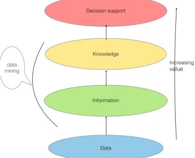
Figure 1. Value chain of Information Gain

In Figure 1, we depict that the mining of data increases the value of collection of vast amounts of data. When we perform data mining on data, we gain some useful information and eventually we are equipped with a better knowledge and understanding of patterns and regularities in the data. This knowledge helps us to make better and more productive

13

Figure 1 : Value chain of Information Gain

Data mining is gaining importance day by day and it has far applications in various fields, bringing optimisations, increasing the revenues and saving limited resources like medicine, food supply. etc.

1.2 Definition of data mining

Data mining is automatic or semi-automatic process of discovering hidden, previously unknown and usable information or patterns from a large amount of data that go beyond simple analysis. The data is analysed without any expectation on the result. Data mining is often is described as the analysis step of knowledge discovery process.

Following are the distinguishing properties of data mining which makes it different from statistical modelling or simple analysis :

• Automatic or semi-automatic discovery of patterns • Prediction of likely outcome

• Creation of actionable information

• Focus on huge amounts of data in multiple formats

• Data mining can answer questions that cannot be addressed through simple query and reporting and require complex mathematical models

Page 10 of 52 Decision support Knowledge Information Data data mining Increasing value

decisions. Therefore, data mining gives us a lot of gain in the value chain which is in often more than the efforts put to perform data mining. The proper knowledge about the patterns in data is even considered very crucial for making decisions in some special scenarios. Such field of applications for data mining is growing day by day, for example, it has now far-reaching applications with the objective of bringing optimisations, increasing the revenues and saving limited resources like medicine, food supply, etc. It saves us a lot of efforts and time in case of complex decision making situations.

2.2

Definition Of Data Mining

Data mining is a process which starts apparently from vast amounts of unstructured datasets in various formats and from various sources to extract useful and interesting information and patterns for making better and timelier decisions [20]. It is an automatic or a semi-automatic process to provide us some useful information which we cannot derive just by looking at the raw data. It is not only limited to business field but also to artificial intelligence, natural language processing, genome sequencing and many other scientific breakthroughs. Data mining has emphasis on utilising data from a particular domain in order to understand some questions in that domain. For gaining useful information from a specified data domain, it applies various data mining algorithms such as prediction, classification, regression, clustering, association-rule discovery, recognition and so on.

These data mining algorithms can be broadly classified into predictive and descriptive

techniques. Predictive techniques are considered to be more similar to machine learning where a model learns over given data (training and testing) and then predicts new instances of data using the learned model e.g. decision tree classifiers and regressors, bayesian classifiers, neural nets etc. Descriptive techniques merely describe characteristics or patterns in the data and there is no learning or training phase. Examples include association rules, summarisation, generalisation, inductive algorithms, etc.

The process of data mining in itself is an empirical approach that is driven by data and it is an attempt to extract statistical regularities of data [20a]. There are 3 components to this approach: data, representation of data and some methods to capture the regularities in data. Feature is another term given to the representations of input data. Features can be superficial and easy to extract or can be deep and difficult to extract. These features are essential for extracting useful regularities or patterns using some kind of model or algorithms. There is a growing evidence that of all three components, data is the most important [11]. When we apply simple data mining methods to the superficial features and to a lot of data, we require much less effort and such a process is more scalable. The accuracies of data mining models obtained using this approach can be continuously improved by using more data. When we use complex methods to derive equally accurate models from small dataset, the complexity hardness of such methods are very difficult to increase. But more complex methods are not always guaranteed to give us more accurate models using small datasets because there can be case that they have escaped some important data which was essential for outputting the model. Additionally, we can see that such an approach is hardly scalable. Thus, we can argue that using simple methods on large dataset to output simple model is evidently a better and more scalable approach than applying complex methods on small datasets to output complex models.

Now, we are faced with the problem that the data mining and analytics need to deal with burgeoning amounts of data. Data volume, variety, velocity and complexity all present challenges that must be faced to efficiently address this problem [21]. This is apparently beyond the capability of single machines at a reasonable cost. There are various possible solutions for introducing scalability to the data mining algorithms. Parallel and distributed data-mining is one of them. This kind of data-mining can run on a diversified type of clusters of machines. This strategy has two facets: distribution of the data and an execution framework for performing distributed processing. Data-centres or clusters need to find an appropriate architecture in order to be scalable and cost-effective. Cloud-computing is one of the architectural model for clusters which has emerged to be affordable and flexible. It is predominantly used for cases when we need to handle and store vast amounts of data and to execute a particular execution on multiple number of nodes in distributed fashion. It is beneficial for both the service-provider and the service-consumer because of the element of elasticity in cases of varying loads.

2.3

Data Mining Process

Data mining is an analytic process of discovering hidden, previously unknown and usable information or patterns from a large amount of data that go beyond simple analysis [20]. The data is analysed without any expectation on the result. Data mining is often is described as the analysis step of knowledge discovery process. But for the data mining process to work properly, we must know the domain of the data, understand the data and the mining methods. We need to understand the data in order to ensure meaningful data mining results because data mining algorithms are often sensitive to specific characteristics of the data: outliers (data values that are very different from the typical or expected values), irrelevant columns, columns that vary together, data coding and data that are chosen to be included or excluded.

Figure 2. Data mining process [22]

15

Figure 2: Data mining process

Figure 2 shows a iterative nature of data mining process where the focus of models is narrowed in the next iteration. Data mining is the most essential step of knowledge discovery in databases.

1.3 Data Mining categories and methods

Data mining methods can be broadly classified into descriptive and predictive. The former describes the data in a concise summarised manner and presents the general interesting properties and patterns; whereas the latter constructs one or a set of models using the past values and predicts the behaviour of new data sets.

Page 11 of 52

Problem Definition

Data Gathering and Preparation

Model Building and Evaluation

Figure 2 shows the general steps in a data mining process. Such a process is iterative in nature which means that the data mining results trigger new questions where the focus of models is narrowed in the next iteration. The first step is to identify the objectives and the requirements and reformulate them into a data mining problem. The following step is to access the data and identify those datasets which addresses the data mining problem well. The input data should be meaningful for the target application. This step is indispensable for improving the data quality which can subsequently improve the information obtained through data mining. It might also involve tasks like data sampling, cleaning and transformation. In model building and evaluation stage, we apply various modelling techniques and finally evaluate how well the model satisfies our initial problem statement. The last stage of knowledge deployment is to apply the model in the real-world targets to obtain the actionable information that we aimed for initially.

2.4

Data Mining Methods And Its Categories

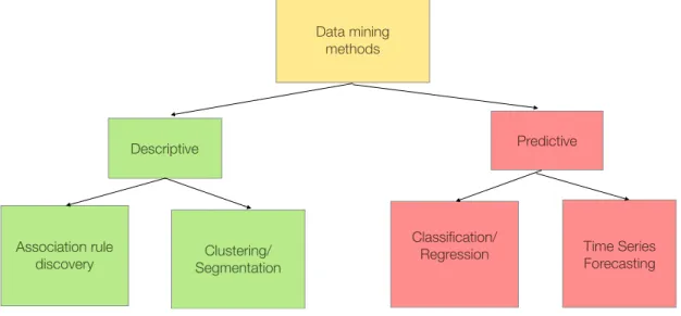
Like mentioned above, data mining methods can be broadly classified into descriptive and predictive. The former describes the data in a concise summarised manner and presents the general interesting properties and patterns; whereas the latter constructs one or a set of models using the past values and predicts the behaviour of new datasets. Figure 3 shows the categorisation of data mining methods and the popular methods in the respective categories.

Figure 3. Data mining methods and its categories

Association-rule discovery or frequent pattern mining searches recurring relationships in

a given data. It discovers interesting associations and correlations between itemsets in our data [23]. Typically, association rules that do not satisfy the minimum support and the confidence are discarded as uninteresting patterns. They are used to derive interesting statistical correlations between attribute-value pairs. This data mining technique is widely used in recommender systems by large e-commerce and online shopping companies like Amazon, Zalando, eBay, etc which we come across in our daily lives. There is a collection

16

1. Association rule discovery is intended to identify strong association relationships or correlations or rules among set of items. Based on the concept of strong rules, Rakesh Agrawal et al.[20] introduced association rules for discovering regularities between products in large-scale transaction data recorded by point-of-sale (POS)

systems in supermarkets.

2. Clustering/Segmentation aims to group a set of objects into k clusters such that

objects in the same cluster are more similar and very different from objects of other

clusters.

3. Classification/Regression computes a classification model using training data whose field attributes and the class label is known. Classification uses this model to predict

the class label for new objects using the field attributes.

4. Time-Series Forecasting is used to predict future values based on previously observed

values.

1.4 Problem Description

First we need to discuss which is better: better algorithms or more data? The

Unreasonable effectiveness of Data, by Norvig et.al [21] shows that for every increase in

order of magnitude of data you have, it beats all improvements in algorithms. Most of the data mining algorithms cannot be solved by neat, concise mathematical formulas. Instead, the best approach appears to be to embrace the complexity of the problem domain and address it by harnessing the power of data. [22] actually performed experiments that demonstrated that simple algorithms with more data actually

outperforms more efficient and elegant algorithms with smaller data sets. [23] also

supports the view that it is worthwhile to look for more data instead of searching for a better classifier. They mention explicitly that the huge amount of data they were able to generate was one of the key factors in their success while classifier itself was a simple random decision forest. [24,25] also points out that it is better to concentrate more on data acquisition rather than fine tuning the algorithms. This is one way to see the problem

Data mining methods

Descriptive Predictive

Association rule

discovery _SegmentationClustering/

Classification/

Regression Time Series Forecasting

of algorithms that implement frequent patten mining. Apriori is one of the foremost algorithm proposed by R. AGRAWAL and R. SRIKANT [24] for mining frequent itemsets for Boolean association rules [23]. This algorithm implements a level-wise iterative searching where the prior knowledge of frequent itemsets in the previous iteration is utilised to reduce the search space for candidate itemsets in the current iteration. This typically requires several passes to the original database. There are several optimisations to this algorithm but their discussion is beyond the scope of this work. Another novel implementation for this

data mining is frequent pattern growth (FP-growth) which employs a divide-and-conquer

tactic to build a frequent pattern tree which contains the itemset association information.

The whole set of transactions are then partitioned into smaller sets each corresponding to one frequent itemset in the tree. The tree grows in similar fashion. The advantage of this approach is elimination of candidate itemsets generation step in every iteration.

Clustering or Segmentation is also a non-predictive technique that aims to group a set of

objects into k clusters such that objects in the same cluster are more similar and they are

very dissimilar from objects of other clusters. Clustering is called as unsupervised learning

because it organises the observed data into meaningful taxonomies, groups or clusters that are initially unknown or not pre-defined [25]. It implies that the training data do not need to

have the class labels. That’s why it is sometimes also referred as automatic classification.

Clustering itself is not an algorithm but refers to a general data mining task which can be implemented by using various algorithms [26]. These algorithms can use various schemes for clustering like distance-based, partitioned-based, hierarchical, density based and model-based clustering. Discussion of such algorithms in detail is beyond the scope of this work.

Classification and regression are two main predictive data mining techniques or methods

that we will discuss in more detail as they are the main focus of our work. Classification is

a data mining method where it learns a predictive model or a function by analysing a set of properly labeled training examples. The derived model is then used to predict the class

labels for new data for which the class label is previously unknown. The term classification

is used when it predicts categorical (discrete, unordered) class labels. It is rather called

regression when the target class labels have continuous values [23]. Both the predictive

techniques are a two-step procedure, comprising of a learning step (to learn a predictive

model or a function) and the application step (where the derived model is used to predict

class labels of given data). The second step is also popularly called as scoring in data

mining literature. This is depicted in Figure 4 where testing or evaluation of output model is rather optional (shown by dotted line).These techniques are also known as supervised learning techniques because the training phase involves training data whose target or predicted labels are previously known. Therefore, the training data should have special characteristics when being applied to these data mining methods. One part of the training example is called explanatory (independent) variable which is grouped together to form a feature vector. The other part is the dependent variable or the predicted class label. In data mining terminology, the feature vector is said to be composed of attributes or features.

(b)

Figure 4. Two-step classification and regression data mining [23]. (a) Learning step (b) Testing and application step

Typically, the first step of classification or regression is to learn the mapping y —> f(X) or the

function y = f(X) that can predict the associated class label y of a given training record X. In

other words, we aim to find classification rules which establish some kind of relationship between the feature vector and the predicted class label. However, this mapping can be represented using a variety of knowledge output representations like classification rules, decision trees or just mathematical formulae. In the second step, we can also measure the accuracy of the predictor model. For this purpose, a set of testing examples are formulated and then the accuracy of the model is derived by the percentage of test set examples that are correctly classified by the model.

For our work, we have chosen classification and regression data mining methods which uses decision tree model as a predictive model. Decision tree models, where the target class labels can only have discrete and finite set of values (categorical values), are called

classification trees [26a]. Decision trees, where the target labels can take continuous

values (typically real numbers), are called regression trees [26a]. We will use the term

decision tree classifiers and decision tree regressors for the corresponding

classification and regression methods to build the decision tree models. We will use an

umbrella term decision tree learning for both methods.

Training data Classification or Regression Algorithm Classification rules or Decision trees or a formulae evaluation scoring Testing data Classification rules or Decision trees or a formulae New Data evaluation scoring (a)

Decision tree is a flowchart-like tree structure where each leaf or terminal node represents the class label or a probability distribution over the set of class labels while each non-leaf or internal node represents a test on an attribute and the branch depicts the result of the test. Therefore, each non-terminal node is labeled with an input feature and the branches from this node is labeled with the possible values of the feature. We have given an example to illustrate the decision tree model in Figure 5. This decision tree learning models the classification rules for the data mining problem: “Whether a customer buys a smartphone?” We have used various features or attributes like age, salary and pension as a test parameter to divide the customer set into two class labels: yes or no.

Figure 5. Decision tree for the date mining goal: “buy a smartphone”

Now, one can easily argue that why we have chosen decision tree learning as a specific data mining algorithm to be parallelized using the MapReduce. This question can be reformulated as: “Why decision tree classifiers and regressors are so popular?” First of all, the construction of decision trees does not require any prior knowledge of the data domain. This means that they are able to handle all kinds of data: both numerical and categorical. They do not feature scaling, data normalisation or dealing with the missing values. They are also able to capture non-linearities and feature interactions. Decision models are rather simple and easy to understand and interpret.

There are several specific algorithms that implement decision tree learning. Iterative Dichotomiser (ID3) is the seminal algorithm invented by J. ROSS QUINLAN, to generate decision trees [27]. ID3 is a precursor for a better algorithm called as C4.5, which was again developed by QUINLAN [28]. Around the same time, group of statisticians (L. BREIMAN, J. FRIEDMAN, R. OLSHEN, and C. STONE) developed a new decision tree algorithm called as Classification and Regression Trees (CART) [29]. Albeit being developed independently, all these algorithms yet follow a similar approach to learn decision trees.

19 evaluation scoring age ? young middle aged retir ed yes salary? pension? yes No high low high low yes No

All three algorithms employ a greedy (also known as non-backtracking) strategy where decision trees are built in a top-down induction and recursive partitioning of data in a divide-and-conquer way [23]. The algorithm proceeds by the recursive partitioning of the training set by selecting a best split candidate or an attribute that maximises the homogeneity of the target labels of training subsets at each child node. In other words, it maximises the value addition to the prediction.The measure of homogeneity or purity of target labels for a set of training tuples at child nodes can be expressed by various statistical properties knows as gini index, entropy and variance. They are the heuristics for splitting criteria. Gini index and Entropy are strictly used for classification trees whereas variance is used for regression trees. When we use gini index, the tree is strictly binary but entropy is able to output multiway trees. Information gain refers to the difference between the purity of child nodes and the parent node. So an attribute is considered as a best split candidate when it maximises the information gain. The node is then labeled with this best split attribute and branches are grown out of this node. If the splitting attribute is a discrete value, a branch is created for each known unique value of this attribute. The training data is partitioned by putting tuples having the same value of the attribute to the corresponding branch. If the splitting attribute is continuous-valued, there are two possible outcomes each corresponding to the attribute values below and above the splitting point. This splitting point is implicitly calculated when calculating best split candidate. In practice, the splitting point is often taken as the midpoint of two known adjacent values of the continuous

attribute and therefore may not actually be a preexisting value of the attribute from the

training data [23]. The recursive partitioning terminates when all the training tuples in the node have same class labels (completely homogeneous) or there is no significant information gain or there are no remaining attributes on which data can be partitioned. In the end, a decision tree is returned.

Classification and regression trees work in a similar way but they differ in the use of impurity measures: classification use gini and entropy while regression use variance. Moreover, they also differ in the representation of the leaf nodes: classification tree uses the most commonly occurring class label as a leaf node whereas regression uses the average value of all the target values in the leaf node. However, decision tree learning algorithms might suffer from overfitting problem and create over-complex trees that do not generalise properly due to some anomalies in the training data such as outliers or noise. This problem of overfitting is rectified by a pruning approach where pruned trees tend to be smaller and less complex. There are two types of pruning: pre-pruning and post-pruning. Pre-pruning halts the construction of tree at earlier stages. This can be done by specifying the maximum depth of the tree or by specifying a minimum threshold for information gain. If the information gain is below this threshold, the leaf nodes are constructed. In this case, leaf nodes contain the most commonly occurring class labels or the average value of target variables. Post-pruning removes sub-trees from a fully-grown tree by replacing them with a leaf node which is labeled with the most frequently occurring class among the subtree being replaced. The criteria for selecting sub-trees to be pruned is the error rates of prediction and the improvement in this error rate after pruning the tree.

3.

MapReduce Concepts

Google MapReduce [15] was the first successful attempt to implement distributed computing on a cluster of low-end cheap commodity servers while hiding the system level details from the programmers. Programmers need to focus only on what computations are to be performed and they don’t need to bother about how computations are actually distributed. The basic idea behind MapReduce is to move the processing closer to the data and to spread the data across the various nodes in the cluster. This is in contrast to the conventional data processing models where data is moved to the processing nodes. The complex task of managing the data is done automatically by the underlying distributed file system called GFS (Google File System). Nowadays, the term MapReduce can refer to three different but related concepts. First, it can refer to the distributed programming model, second it can refer to the runtime environment that facilitates the distributed computations and lastly it can refer to the software implementations like Google, open-source Hadoop, MapR, Apache Spark etc. The first concept is relevant for our work. The term MapReduce refers to distributed data processing model rather than to a specific implementation for our work.

3.1

MapReduce Paradigm

MapReduce programming model derives its inspiration from functional programming models like LISP and ML. The key concept of functional programming is that the higher-order functions can accept other functions as arguments. Just as map and reduce functions in the functional programming languages like LISP, we have two stage processing structure

in MapReduce. First stage is a embarrassingly parallel map step which is basically a

transformation stage where it reads and processes discrete chunks of data called as ‘splits’ in parallel. The second stage is called reduce stage where the sorted output from the map step is aggregated and stored back to the permanent storage. So the process of converting complex algorithms into equivalent MapReduce algorithms is to express all the computations (those that can be parallelised) in the original algorithm using map and reduce functions only.

3.2

Pre-Requisites

The first and the foremost task is to determine if a particular algorithm can be parallelised

and implemented using MapReduce paradigm. CHU ET AL. have given a generalised

approach to test whether a particular algorithm can be adopted to MapReduce. They have proved that any algorithm that satisfies the “Statistical Query Model” can be expressed in a summation form. Moreover, MapReduce is one of the easiest way to express this summation form and write the corresponding program. Algorithms that compute enough statistics or gradients satisfy this model. They have shown that if the summations are batched, it can be easily implemented using two stage process: first stage to compute the statistics and second stage to sum all of them [13]. Now, we will enumerate some of the general restrictions with respect to the input data to the MapReduce processing. Data should have “Write Once Read Many” (WORM) characteristics because such data fulfil the

necessary condition for being processed in parallel fashion without the need for mutexes. The tuples in data should not have any dependencies on other tuples so that out-of-order processing is possible. In order to fully exploit the potential of MapReduce, data-set should be very large because MapReduce is an execution framework that has been designed for processing large-scale data. MapReduce is a partial parallel algorithm because the input of

the map and reduce should always be of the form <key, value>. This key-value structure

is imposed on the input when the data tuples are read from the underlying special Distributed file systems such as HDFS, GFS by the MapReduce run-time.

3.3

Architecture And Programming Model

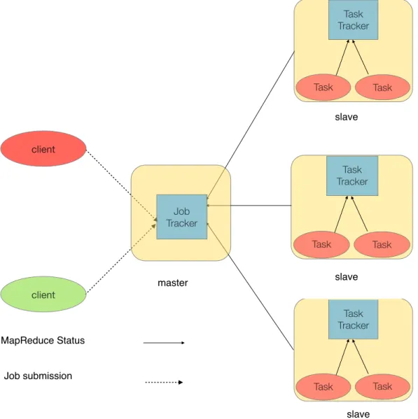
The architecture of MapReduce programming model, as proposed in [15], is of master-slave paradigm. One of the nodes is a special node: master node. It has the responsibility of assigning map and reduce tasks to the slave nodes, monitoring task progress on each of the slaves nodes, periodically detecting slave node failures and restarting failed map and reduce tasks preferably on alive slave nodes which have the replicated data. Slave nodes only run map or reduce tasks and periodically inform the progress of the task completion back to the master node. Figure 6 shows the original architecture of MapReduce and its execution flow. The client program forks a master process on the master node and slave processes on other slave nodes. From this point, master node assumes the responsibility of scheduling the map and reduce tasks on slave nodes. Slave nodes execute the map and the reduce tasks which are assigned to them by the master node. Before the reduce tasks can be started, all the map tasks should be finished. This can be viewed as a synchronisation step between map and reduce tasks. Map tasks send the output to the reduce tasks by using a distributed shuffle and sort operation. Combiner and partitioner steps are optional and are basically optimisations. Combiner reduces the size of map outputs by performing the local reduce. Combiner reduces the size of shuffle data between map and reduce tasks. Partitioner divides the map output into number of reducers. Various kind of partitioning schemes can be employed like hash partitioning. In reduce step, all the values with same key are combined and the merged results are stored back to the DFS storage. The reduce results are first sorted by their keys before they are stored to DFS. The key aspect of the MapReduce programming model is that if every Map and Reduce is independent of all other ongoing Maps and Reduces, then the operation can be run in parallel on different keys and values [30]. One of the most important aspect of MapReduce processing model is that it runs the map tasks on the nodes where the data lives. This ensures that there is no or very little movement of data between nodes and preserves the

valuable network bandwidth. This property is called as data locality optimisation. All the

independent computations need to be specified in 2 kinds of functions: map and reduce.

We will now give a general definition of map and reduce transformations:

Map. A map transform is provided to transform an input data row of key and value to an

output list containing zero or more (key,value) pairs: map(key1,value) -> list<key2,value2>

Reduce. A reduce transform is provided to take all values for a specific key, and generate a

Figure 6. Overall MapReduce programming model architecture [15]


23

Fig Overall MapReduce architecture and processing model

Page 15 of 52 Master 1.fork 1.fork 1.fork HDFS Storage HDFS Storage

split split split

map map map

combiner partitioner split map reduce HDFS Storage

split split split

map map map

combiner partitioner split map s l a v e / worker s l a v e / worker s l a v e / worker 2.assign map 2.assign map 2.assign reduce distributed sort/ shuffle 1.fork 3.read client program

4. Hadoop

This section gives an overview to Hadoop, an open-source project under Apache Software Foundation and distributed under Apache License 2.0 [4]. It is necessary to understand the basics of Hadoop because we have used Hadoop based cluster to perform our experiments later. There are numerous reasons to use this framework to build the cluster. While MapReduce software framework from Google is proprietary, Hadoop is an open source, the most accessible and the most mature implementation of MapReduce. In Hadoop, data storage and computation both live on the same machines within the cluster. By leveraging this proximity of data, hadoop is capable of efficiently processing large volumes of data. Therefore, we can leverage the data mining analytics easily and cost effectively using Hadoop. Since it is written in Java, it can run on any platform running JVM. It implies that there are no special requirements on machines that will comprise the cluster. Building up distributed systems requires coordination of large number of machines, large-scale data storage and analysis and Hadoop provides very simple and easy-to-use tools for that purpose. All the modules in Hadoop framework are designed to automatically handle hardware failures. This fault-tolerance is made possible by the automatic and efficient data replication in Hadoop. There are 2 basic modules in Hadoop which are essential to understand for this work: Hadoop Distributed File System (HDFS) module for distributed data storage and MapReduce module for distributed data processing. We have used HDFS for storing large-scale data in our experiments. Although, we will see later that we have not used the MapReduce processing framework of Hadoop, we need to understand this original and the most mature MapReduce framework because it is the reference framework for other advanced and optimised MapReduce frameworks. It is of immense help to understand the fundamentals of Hadoop’s MapReduce processing, so that we can later compare this with the optimised MapReduce framework (which is Apache Spark) that we have used for our work. We need to have a basic idea about the original MapReduce so that we can comprehend the optimisations that are implemented in other MapReduce-like frameworks.

Hadoop has namely two major versions: Hadoop 1.x and 2.x. The 2.x version is scalable up to 10,000 nodes whereas 1.x version is scalable only up-to 4000 nodes because the newer version has better cluster management capabilities and provide fine-grained memory management capabilities. 1.x uses slot-based mechanism for memory allocation and it leads to under-utilisation of overall cluster memory. 2.x uses container-based memory allocation which is more flexible. Nevertheless, both versions have improved tremendously in terms of scalability, reliability, manageability and performance over incremental releases.

4.1

HDFS - Hadoop Distributed File System

There are several distributed file systems that has been in use for several decades, then why do we need a special DFS like HDFS? Let us take an example of the most ubiquitous file system: NFS (Network File System) [17]. It has been so popular because of its major advantage being the location transparency of files. All the file commands for local filesystem also works on files hosted on NFS as if they are locally hosted. But there are several limitations of NFS. The first problem is that all files belonging to one NFS volume should

reside on a single machine. Thus the size of single machine is the upper limit of the size of a NFS volume. If there are large number of clients requesting files from this single NFS volume, the machine will be probably overloaded. Moreover, it does not provide any out-of-the-box reliability guarantees because there is no replication supported. The primary requirement is that distributed File system should tolerate node failures without any data loss. Now we will see how the unique design of HDFS that solves all the shortcomings of NFS.

4.1.1 Design of HDFS

The architecture of HDFS is described in the original paper from Yahoo! Inc. [31], which is based on the design of GFS [32]. HDFS can store large amounts of data (in order of terabytes or petabytes) and the size of files is not limited by the size of single DFS machine because it stores files by breaking them into blocks of fixed sizes (128 MB by default) which might typically reside on different machines across the cluster. It also provides automatic fault-tolerance and handles the node failures by replicating the blocks on various machines in an efficient manner. The size of the blocks is usually very large as compared to traditional filesystem blocks so that seek times are much smaller as compared to time for reading data from the disks. Therefore, it gives very high throughput and performance in case of applications that require long sequential reads from the disks. It is also designed to use commodity disk drives because it provides automatic fault tolerance in case of disk failures. Hadoop has the fundamental flexibility to handle unstructured data regardless of the data source or format. Additionally, disparate types of data stored on unrelated systems can all be deposited in the Hadoop cluster without the requirement to predetermine how the data will be analysed. But the design of HDFS which makes it highly scalable and gives very high performance also makes it limited to a particular class of applications. It is specially suitable for data which has Write Once and Read Many (WORM) and strong independent properties. Applications which require very instant seek accesses are not suitable for HDFS storage. But the data locality optimization of HDFS makes it very suitable for any kind of MapReduce applications. Data locality optimisation implies that the blocks are stored in such a manner that there are minimal movements of blocks between machines belonging to the same rack and even lesser block movements between machines in different racks. HDFS follows a rack-aware architecture.

In Figure 7, we illustrate the architecture of HDFS using an example where there is one master node and 3 slave nodes.The architecture of HDFS is based on master-slave design

[33]. The master node is called namenode whereas the slave nodes are called datanodes

[34]. Namenode holds the filesystem tree and its metadata persistently on a local disk but it stores the metadata about block locations in memory. Therefore, namenode needs typically more memory than data nodes. Large size of HDFS blocks also means that there will be relatively low amount of metadata per file as the memory needed by namenode is typically determined by total number of blocks in the HDFS. Datanodes manages, store and retrieve blocks in a HDFS directory as directed by the client or namenode. In Figure 7, we show that a read or a write client can do the respective operations on any slave or master node but it first needs to consult the namenode. In case of read operation, the read client needs to fetch the metadata information about the physical location of the blocks and their replicated

versions on data nodes from namenode. In case of a write operation, the write client informs the namenode about its intention to write a block of a file. Namenode replies back with the address of the datanode where the requested block can be stored. Write client writes the block to the specified datanode. Datanodes are then responsible for replicating the particular block by a replication factor value specified for the HDFS system. In the given example, the replication factor is 2. This cycle repeats for next blocks until all the blocks of file are written to the HDFS ensuring that the required replication factor is always fulfilled.

Figure 7. HDFS architecture and the flow of execution for read and write operations [34]

4.2

MapReduce Framework

In this sub-section, we develop a comprehensive understanding of fundamentals of MapReduce processing framework [35]. This specifically refers to the original implementation by Hadoop. We will describe only the important characteristics of this framework which is important for building a concept about MapReduce distributed

programming model. In Hadoop, a MapReduce jobis the highest unit of abstraction of work

in Hadoop and it is submitted by a job client. The job consists of three minimal

components: specification of input and output paths, definition of map and reduce tasks

and various other configuration parameters. For this purpose, JobConf is the primary

3.1 HDFS (Hadoop Distributed File System)

Design

The architecture of HDFS is described in the original paper from Yahoo! Inc [29], which is based on the design of GFS [33]. HDFS can store large amount of data (terabytes or petabytes) and the size of files is not limited by the size of single DFS machine because it stores a file by breaking it into blocks of fixed sizes (64 MB by default) which might typically reside on different machines across the cluster. It also handles the node failures

Page 17 of 52 Metadata: Files block ID usr/hadoop/ file1 1,2,5 usr/hadoop/ file2 3,4 5 4 1 3 2 3 Datanode 1 Datanode 2 Read Client 1. request metadata 3. Read 2 4 1 5 2. Metadata info 4.Replicate 3. read master slave slave slave Datanode 3 Namenode write Client 1. want to write block 5 of file1

2. Write to datanode 2