Multiple Classifiers Applied to Multisource
Remote Sensing Data
Gunnar Jakob Briem, Associate Member, IEEE, Jon Atli Benediktsson, Senior Member, IEEE, and
Johannes R. Sveinsson, Senior Member, IEEE
Abstract—The combination of multisource remote sensing and geographic data is believed to offer improved accuracies in land cover classification. For such classification, the conventional para-metric statistical classifiers, which have been applied successfully in remote sensing for the last two decades, are not appropriate, since a convenient multivariate statistical model does not exist for the data. In this paper, several single and multiple classifiers, that are appropriate for the classification of multisource remote sensing and geographic data are considered. The focus is on multiple classi-fiers: bagging algorithms, boosting algorithms, and consensus-the-oretic classifiers. These multiple classifiers have different charac-teristics. The performance of the algorithms in terms of accuracies is compared for two multisource remote sensing and geographic datasets. In the experiments, the multiple classifiers outperform the single classifiers in terms of overall accuracies.
Index Terms—Bagging, boosting, consensus theory, multiple classifiers, multisource remote sensing data.
I. INTRODUCTION
D
ATA FUSION of multisource remote sensing and geo-graphic data for classification purposes has been an im-portant research topic for more than a decade. In such fusion, different types of information from several data sources, e.g., Landsat Thematic Mapper data, radar data, elevation data, and slope data, are used in order to improve the classification ac-curacy as compared to the acac-curacy achieved by single-source classification.A major observation in previous research on multisource classification is that conventional parametric statistical pattern recognition methods are not appropriate in classification of such data, since in most cases they cannot be modeled by a convenient multivariate statistical model [1], [2]. Therefore, other methods have been looked at.
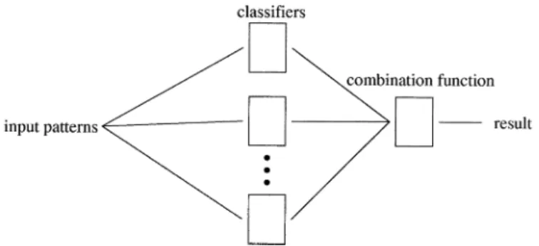
Here, we are interested in the use of an ensemble of classifiers or multiple classifiers (a schematic representation of which is shown in Fig. 1) for classification of multisource data. Tradition-ally, in pattern recognition, a single classifier is used to deter-mine which class a given pattern belongs to. However, in many cases, the classification accuracy can be improved by using an ensemble of classifiers in the classification. In such cases, it is
Manuscript received September 26, 2001; revised May 17, 2002. This re-search was supported in part by the Icelandic Rere-search Council and the Rere-search Fund of the University of Iceland.
G. J. Briem was with the Department of Electrical and Computer Engineering, University of Iceland, Reykjavik IS-107, Iceland. He is now with Dimon Soft-ware, Reykjavik IS-105, Iceland.
J. A. Benediktsson and J. R. Sveinsson are with the Department of Electrical and Computer Engineering, University of Iceland, Reykjavik IS-107, Iceland.
Digital Object Identifier 10.1109/TGRS.2002.802476
Fig. 1. Schematic diagram of a multiple classifier.
possible to have the individual classifiers support each other in making a decision. The aim is to determine an effective combi-nation method that makes use of the benefits of each classifier but avoids the weaknesses.
In this paper, the performance of three types of multiple clas-sifiers are investigated in terms of classification of multisource remote sensing and geographic data. The paper is organized as follows. First, multiclassifier systems are discussed with a spe-cial emphasis on the recently proposed bagging and boosting algorithms and statistical consensus theory. Experimental re-sults for the multisource remote sensing and geographic datasets are given in Section III. Finally, conclusions are drawn in Sec-tion IV.
II. MULTICLASSIFIERSYSTEMS
Several methods have been proposed to combine multiple classifiers [3]–[5]. Wolpert [3] introduced the general method of stacked generalization where outputs from classifiers are com-bined in a weighted sum with weights that are based on the in-dividual performance of the classifiers. Tumer and Ghosh [4] have also shown that substantial improvements can be achieved in difficult pattern recognition problems by combining or in-tegrating the outputs of multiple classifiers. Benediktsson et
al. combined classifiers using neural networks [6], [7] and
im-proved their overall accuracies as compared to the best results of the single classifiers involved in the classification.
The theory of multiclassifier systems can be traced back at least as far as 1965 [8], [9]. Currently, two of the most used mul-ticlassification approaches are boosting [10], [11] and bagging [12]. Both these approaches are based on manipulating training samples. In contrast, statistical consensus theory is based on treating data sources separately, and it uses all the training data only once. All three approaches are discussed briefly below.
A. Boosting
Boosting is a general supervised method that is used to increase the accuracy of any classifier. Several versions of boosting have been proposed, but we will concentrate on AdaBoost [11], which was proposed in 1995. In particular, we will use the AdaBoost.M1 method, which can be used on classification problem with more than two classes. This version of the AdaBoost algorithm is shown as follows.
Input: A training set S with m samples, where each sample x is of class !, base classifier I, and number of classifiers T.
1. S = S and weight(x ) = 1 for j = 1 . . . m (x 2 S) 2. For i = 1 to T {
3. C = I(S )
4. = 1=m weight(x )
5. If > 0:5, set S to a bootstrap sample from S with weight(x) = 1 8 x 2 S and go to Step 3 If is still >0.5 after 25 iterations, abort! 6. = =(1 0 )
7. For each x 2 S{ if C (x ) = ! then weight(x ) =weight(x ) 1 }
8. Norm weights such that the total weight of S is m
9. }
10. C (x) = arg max log(1= )
Output: The multiple classifier C .
In the beginning of AdaBoost, all samples have the same weight, , thus forming a uniform distribution , and they are used to train the classifier . Then, the samples are reweighted in such a way that the incorrectly classified samples have more weight than the correctly classified ones. Based on this new distribution, the classifier of the next iteration is trained. The classifier of iteration , , is therefore based on the distribution calculated in iteration .
Iteration by iteration, the weight of the samples that are cor-rectly classified goes down. Therefore, the algorithm starts con-centrating on the difficult samples. At the end of the procedure, weighted training sets and base classifiers have been gen-erated.
It is recognized that not all base classifiers accept a weighted set of samples. In such cases, instead of supplying the distribu-tion directly to the base classifier, a set of samples is chosen from in accordance with by replacement. This is similar to the bootstrapping performed in the bagging method discussed next, except that the distribution generally is not uniform.
If the classification error is greater than 0.5, an attempt is made to decrease it by bootstrapping. If the classification error stays above 0.5, then the procedure is stopped (in failure). A demand is made, therefore, on the minimum accuracy of the base classifier, which can be of considerable disadvantage in multiclass problems.
The main advantage of AdaBoost is that in many cases it in-creases the overall accuracy of the classification. Many practical classification problems include samples that are not equally dif-ficult to classify, and AdaBoost is suitable for such problems.
AdaBoost tends to exhibit virtually no overfitting when the data are noiseless. Other advantages of boosting include that the al-gorithm has a tendency to reduce both the variance and the bias of the classification [11], [13]. On the other hand, AdaBoost is computationally more demanding than other simpler methods. Therefore, it is dependent on the classification problem whether it is more valuable to get increased classification accuracy or to obtain a simple and fast classifier. Another problem with Ad-aBoost is that it usually does not perform well in terms of accu-racies when there is noise in the data.
B. Bagging
Bagging is an abbreviation of bootstrap aggregating. Boot-strap methods are based on randomly and uniformly collecting samples with replacement from a sample set of size . The bagging algorithm (which, like AdaBoost, is supervised) was proposed in 1994 [12] and constructs many different bags of samples by performing bootstrapping iteratively, classifying each bag, and computing some type of an average of the classifications of each sample via a vote. Bagging is in some ways similar to boosting, since both methods design a collection of classifiers and combine their conclusions with a vote. However, the methods are different. For example, because bagging always uses resampling instead of reweighting, it does not change the distribution of the samples (does not weight them), so all classifiers in the bagging algorithm have equal weights during the voting. It is also noteworthy that bagging can be done in parallel, i.e., it is possible to prepare all the bags at once. On the other hand, boosting is always done in series, and each sample set is based on the latest weights. The bagging algorithm can be written as follows.
Input: A training set S with m samples, where each sample x is of class ! , base classifier I, and number of bootstrapped sets T.
1. For i = 1 to T{
2. S = bootstrapped bag from S 3. C = I(S )
4. }
5. C (x) = arg max 1
Output: The multiple classifier C .
From the above, it can be seen that bagging is a very simple algorithm. Each classifier is trained on a bootstrapped set of samples from the original sample set . After all classi-fiers have been trained, a simple majority vote is used, but if more than one class jointly receives the maximum number of votes, then the winner is selected using some simple mecha-nism, e.g., random selection. For a particular bag , the prob-ability that a sample from is selected at least once in tries
is . For a large , the probability is
approxi-mately , indicating that each bag only includes
about 63.2% of the samples in . If the base classifier is un-stable, i.e., when a small change in training samples can result in a large change in classification accuracy, then bagging can im-prove the classification accuracy significantly. If the base classi-fier is stable, e.g., like a k-NN classiclassi-fier, then bagging can reduce
the classification accuracy because each classifier receives less of the training data.
The main advantage of the bagging algorithm is that it can in-crease the classification accuracy significantly if the base classi-fier is properly selected. The bagging algorithm is also not very sensitive to noise in the data. The algorithm uses the instability of its base classifier in order to improve the classification ac-curacy. Therefore, it is of great importance to select the base classifier carefully. This is also the case for boosting, since it is sensitive to small changes in the input signal. Bagging reduces the variance of the classification, just as boosting does, but in contrast to boosting, bagging has little effect on the bias of the classification.
C. Consensus Theory
Consensus theory is not based on manipulating the training data like bagging and boosting. Consensus theory [6], [14] in-volves general procedures with the goal of combining single probability distributions to summarize estimates from multiple experts, with the assumption that the experts make decisions based on Bayesian decision theory. The combination formula obtained is called a consensus rule. The consensus rules are used in classification by applying a maximum rule, i.e., the summa-rized estimate is obtained for all the information classes, and the pattern X is assigned to the class with the highest summarized estimate. Probably, the most commonly used consensus rule is the linear opinion pool (LOP), which is based on a weighted linear combination of the posterior probabilities from each data source. Another consensus rule, the logarithmic opinion pool (LOGP), is based on the weighted product of the posterior prob-abilities. The LOGP differs from the LOP in that it is unimodal and less dispersed. Also, the LOGP treats the data sources inde-pendently.
The weighting schemes in consensus theory should reflect the goodness of the input data. The simplest approach is to give all the data sources equal weights. Also, reliability measures that rank the data sources according to their goodness can be used as a basis for heuristic weighting [6]. Furthermore, the weights can be chosen to not only weight the individual sources but also the individual classes. For such a scheme, both linear and nonlinear optimization can be used.
III. EXPERIMENTALRESULTS
Two experiments were conducted on multisource remote sensing and geographic data using bagging, boosting, and consensus-theoretic classifiers. To obtain baseline results for the multiple classifiers, several single classifiers were applied to the data. These include the minimum Euclidean distance (MED) classifer, Gaussian maximum likelihood (ML) classi-fier, and conjugate-gradient backpropagation (CGBP) [6] with two and three layers. The base classifiers that were used for bagging and boosting were also trained as single classifiers on the data. These base classifiers were as follows:
1) decision table with a ten-fold cross validation for feature selection and termination of search for the best feature set after 15 nonimproving subsets [15];
2) j4.8 decision tree [16] (an implementation of the C4.5 revision eight-decision tree [17]);
TABLE I
TRAINING ANDTESTSAMPLES FORINFORMATIONCLASSES IN THE EXPERIMENT ON THECOLORADODATASET
Fig. 2. Colorado data. Average spectra for three forest type classes. The first four features are the Landsat MSS data, followed by elevation, slope, and aspect respectively.
3) simple classifier 1R with minimum bucket size of eight [18], which only uses one feature when it determines a class.
In summary, the single classifiers applied to the datasets were the following:
• minimum Euclidean distance (MED); • maximum likelihood (ML);
• conjugate-gradient backpropagation (CGBP); • decision table;
• j4.8 (an implementation of the C4.5 decision tree); • 1R (classification based on one feature).
In the results below, the average accuracy is defined as the av-erage of the classification accuracy of each class, regardless of the number of samples in each class. The overall accuracy is defined as the number of correctly classified samples, regardless of which class they belong to, divided by the total number of samples.
TABLE II
TRAININGACCURACIES INPERCENTAGE FOR THEDIFFERENTCLASSIFICATIONMETHODSAPPLIED TO THECOLORADODATASET
A. Colorado Dataset
In the first experiment, classification was performed on a dataset consisting of the following four data sources:
1) Landsat MSS data (four spectral data channels);
2) elevation data (in 10-m contour intervals, one data channel);
3) slope data (0 to 90 in 1 increments, one data channel); 4) Aspect data (1 to 180 in 1 increments, one data
channel).
The area used for classification is a mountainous area in Col-orado. Ground reference data are available with ten ground-cover classes. One class is water; the others are forest types, as specified in Table I. It is very difficult to distinguish among the forest types using the Landsat MSS data alone, since the forest classes show very similar spectral response. A typical example of this is shown in Fig. 2 for the average spectra of three of the forest type classes. For these classes, it is clear that it helps to add the topographic data sources to the Landsat data in order to make the data more distinguishable.
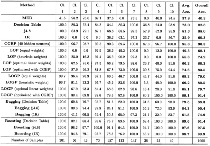
The training accuracies for both single and multiple clas-sifiers are given in Table II. The test accuracies are given in Table III. It was not possible to use the Gaussian maximum likelihood classifier for the Colorado dataset. The covariance matrix, which was computed using the standard unbiased esti-mation on the raw data, became singular for several of the forest type classes because of little variation in the topographic data.
For the LOP and LOGP, ten data classes were defined in each data source. The multispectral remote sensing data sources were modeled to be Gaussian. On the other hand, the topographic data sources were modeled by Parzen density estimation with Gaussian kernels [19], which constructs an average of density functions, centered at each training sample. Several different weighting schemes were used for the LOP and LOGP [6].
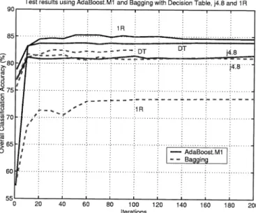
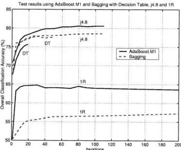
Both bagging and boosting were applied on the raw data and run using the WEKA software provided by the University of Waikato, New Zealand [20]. In the case of bagging, 100 itera-tions were selected for the decision table, ten iteraitera-tions for j4.8, and 200 iterations for 1R. For boosting, the Adaboost.M1 was employed, with 50 iterations for the decision table, 200 itera-tions for j4.8, and 60 iteraitera-tions for 1R. The number of iteraitera-tions was chosen after trying up to at least 300 iterations for j4.8 and 1R and 100 iterations for the decision table. A plot of the overall test accuracies as a function of the number of iterations is shown in Fig. 3. In each case, the ten-class problem was converted into multiple two-class problems, through the use of the
MultiClass-Classifier [20], to make it more tractable for the base
classi-fiers, especially in view of the stringent classification accuracy demand of the AdaBoost.M1 algorithm. As can be seen from Fig. 3, all plots have a knee at 10 to 20 iterations. After that, they improve only slightly.
At first glance, it may seem odd that in the experiments different numbers of iterations were used when bagging and boosting each base classifier (as discussed below). However, the
TABLE III
TESTACCURACIES INPERCENTAGE FOR THEDIFFERENTCLASSIFICATIONMETHODSAPPLIED TO THECOLORADODATASET
Fig. 3. Colorado data. Test accuracies as a function of the number of iterations.
goal was not to compare the computational demands of bagging and boosting each base classifier, but rather to compare them in terms of the highest achievable test accuracies. Therefore, it was decided to use the “optimal” number of iterations for each base classifier instead of using the same number of iterations for all three base classifiers.
TABLE IV
TRAINING ANDTESTSAMPLES FORINFORMATIONCLASSES IN THE EXPERIMENT ON THEANDERSONRIVERDATASET
From Tables II and III, it is apparent, that all three multiple classifier schemes show improvement over the single classifiers (minimum Euclidean distance, decision table, j4.8, 1R, and two-layer conjugate-gradient backpropagation with 40 hidden neurons) in terms of both average and overall accuracies (the ML classifier was not applicable here because of singularity problems). The highest overall and average training accura-cies were achieved by boosting the j4.8 decision tree. How-ever, the highest overall and average test accuracies were ob-tained by boosting the 1R base classifier, which gave far worse training and test accuracies on its own than the other base
TABLE V
TRAININGACCURACIES INPERCENTAGE FOR THEDIFFERENTCLASSIFICATIONMETHODSAPPLIED TO THEANDERSONRIVERDATASET
classifiers. In contrast, bagging the 1R gave poor accuracies. The best overall and average accuracies for consensus-theoretic classifiers were achieved with the LOGP optimized by conju-gate-gradient backpropagation. Those results were comparable in terms of overall accuracies to the best results achieved using bagging.
The classification accuracies for the individual classes are in-teresting in Tables II and III. When 1R is used, it gives extremely low accuracies for classes number 2, 3, 4, 8, and 9. Boosting gives significant improvements to the training and test classi-fication accuracies for all these classes. For example, 1R gives 0% training and test accuracies for class number 9, but boosting the 1R base classifier gives a training accuracy of 100% and test accuracy of 72% for that class. Boosting using other base classi-fiers gives accuracy improvements for all other classes. Bagging also gives improvements in terms of class-specific accuracies but is outperformed by boosting.
B. Anderson River Dataset
In the second experiment, the Anderson River dataset, which is a multisource remote sensing and geographic dataset made available by the Canada Centre for Remote Sensing (CCRS) [21], was used. This dataset is very difficult to classify [6] due to a number of mixed forest type classes.
Six data sources were used:
1) Airborne Multispectral Scanner (AMSS) with 11 spectral data channels (ten channels from 380–1100 nm and one channel from 8–14 m);
2) steep mode synthetic aperture radar (SAR) with four data channels (X-HH, X-HV, L-HH, L-HV);
3) shallow mode SAR with four data channels (X-HH, X-HV, L-HH, L-HV);
4) elevation data (one data channel, where elevation in
meters pixel value );
5) slope data (one data channel, where slope in degrees pixel value);
6) aspect data (one data channel, where aspect in degrees pixel value).
There are 19 information classes in the ground reference map provided by CCRS. In the experiments, only the six largest ones were used, as listed in Table IV. Here, training samples were se-lected uniformly, giving 10% of the total sample size. All other known samples were then used as test samples.
The results of the different classification methods are shown in Table V (training) and Table VI (test). For the single clas-sifier methods in Tables V and VI, the MED and ML showed different characteristics. The MED was not acceptable in terms of classification accuracies, but the ML accuracies were
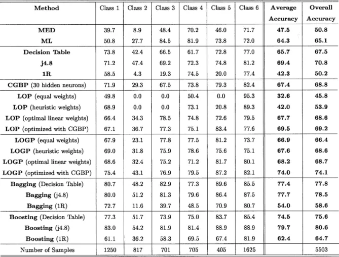
rela-TABLE VI
TESTACCURACIES INPERCENTAGE FOR THEDIFFERENTCLASSIFICATIONMETHODSAPPLIED TO THEANDERSONRIVERDATASET
tively good, especially considering that the data are clearly not Gaussian [21]. The j4.8 method outperformed the other single classifier methods in terms of both training and test accuracies and achieved an overall accuracy for test data of 70.8%. The test accuracy of the decision table was somewhat lower than that of the CGBP neural network, which achieved a test accuracy of 68.8%.
For the LOP and LOGP, six data classes (corresponding to the information classes in Table IV) were defined in each data source. The AMSS and SAR data sources were modeled to be Gaussian, but the topographic data sources were modeled by Parzen density estimation with Gaussian kernels [6]. From the results for the consensus-theoretic methods in Tables V and VI, it is clear that the LOGP optimized with a neural network outperformed all other consensus-theoretic methods in terms of overall and average training and test accuracies. It is note-worthy that the CGBP optimization increased the overall accu-racies of the equally weighted LOGP by approximately 12% (training) and 6% (test), and the LOGP with nonlinearly opti-mized weights outperformed easily the best single-stage neural network classifiers both in terms of training and test accuracies. In contrast, the CGBP-optimized LOP only gave comparable results to the single-stage CGBP with 30 hidden neurons. How-ever, the best CGBP-optimized LOP results were achieved with zero hidden neurons where the best CGBP-optimized LOGP
re-sults were reached with 45 hidden neurons. These rere-sults are not surprising. The LOP is a linear combination of posterior proba-bilities, but the LOGP is nonlinear.
In the case of bagging, 100 iterations were selected for the j4.8, 30 iterations for the decision table, and 700 iterations for 1R. The test accuracies, both for bagging and boosting, as a function of the number of iterations are shown in Fig. 4. The bagging of the decision table and the j4.8 was done directly on the six-class classification problem. However, the 1R classifier had difficulties with the six-class problem, so it was fragmented into multiple two-class problems using MultiClassClassifier, as was done for all cases in the classification of the ten-class Colorado dataset. As can be seen in Fig. 4, the test accuracy seemed to have approximately converged in all bagging cases. Evidently, the bagging algorithm improved on the best training or test results given by LOGP when the j4.8 base classifier is used. This result comes as no surprise, since decision tree clas-sifiers are typical unstable clasclas-sifiers that should perform well in classification by the bagging algorithm. Bagging based on the decision table does almost as well in terms of test accuracies and, in fact, slightly better than bagging based on the j4.8 after 30 iterations.
For boosting, the Adaboost.M1, with 100 iterations for j4.8, was employed. However, after 19 iterations the boosting of the decision table aborted. This demonstrates how strict
Fig. 4. Anderson River data. Test accuracies as a function of the number of iterations.
the demand for 50% accuracy is for multiclass problems. Nevertheless, the MultiClassClassifier was only employed for the 1R base classifier. The fact that MultiClassClassifier was used for all bagging and boosting methods on the Colorado dataset, and the 1R method on the Anderson River dataset, but not for the Decision Table and j4.8 methods on the An-derson River dataset, skews the comparison between different methods somewhat. It is expected that, in general, given enough data and computational resources, better accuracies would be achieved by applying the base classifiers directly on the multiclass problem, instead of multiple two-class problems. However, it was deemed necessary for the ten-class Colorado dataset to split it into multiple two-class problems, and the 1R base classifier could not make a single iteration of the AdaBoost.M1 on the Anderson River dataset without applying the MultiClassClassifier.
The justification for using different numbers of iterations for each method is that our aim was to compare the methods in terms of the highest achievable test accuracies, rather than the computational requirements.
As can be seen from Tables V and VI, the Adaboost.M1 al-gorithm improved on the results given by bagging in the case of the j4.8 classifier, but not the decision table. The j4.8 base classi-fier results are outstanding. These results are the best accuracies achieved for the whole experiment on the Anderson River data. It is of interest to note that the best overall test accuracies were achieved 95 iterations after the training accuracy reached 100%. Similar to the experiment on the Colorado dataset, boosting and bagging, in most cases, gave good improvements on the accura-cies of the single classifiers when looked at on a class-by-class basis. Contrary to the Colorado dataset, boosting and bagging the 1R classifier on the Anderson River dataset did have prob-lems. A plausible reason for these problems is that the 1R base classifier, while giving good results on the seven-feature Col-orado dataset, is too simple to classify the 22 features of the Anderson River dataset based on just one feature.
IV. CONCLUSIONS
In this paper, three multiple classification schemes were investigated. All three schemes performed well and out-performed several single classifiers in terms of accuracies. Therefore, the results presented here demonstrate that multiple classification methods can be considered desirable alternatives to conventional classification methods for classification of multisource remote sensing and geographic data. In particular, the AdaBoost.M1 method yielded the most accurate classifier both in terms of training and test accuracies, when the j4.8 decision tree was used as the base classifier in the case of the Anderson River dataset, and when the 1R method was used as the base classifier in the case of the Colorado dataset. The AdaBoost.M1 did not demonstrate overtraining although it achieved 100% training accuracy. For the Anderson River dataset, the simpler bagging algorithm performed better than AdaBoost.M1 in the case of the decision table base classifier, where the AdaBoost.M1 aborted after only 19 iterations. Bagging does not suffer from the restriction of needing at least 50% accuracy and has the further advantage of needing not as much computational resources as the other methods. The LOGP consensus-theoretic classifier performed well in experiments. Consensus-theoretic classifiers have the potential of being more accurate than conventional multivariate methods in classification of multisource data, since a convenient mul-tivariate model is not generally available for such data. Also, consensus theory overcomes two of the problems with the conventional ML method. First, using a subset of the data for individual data sources lightens the computational burden of a multivariate statistical classifier. Second, a smaller feature set helps in providing better statistics for the individual data sources when a limited number of training samples is available.
ACKNOWLEDGMENT
The Colorado dataset was loaned by R. Hoffer of Colorado State University. The Anderson River SAR/MSS dataset was acquired, preprocessed, and loaned by the Canada Centre for Remote Sensing, Department of Energy Mines, and Resources, of the Government of Canada.
REFERENCES
[1] T. Lee, J. A. Richards, and P. H. Swain, “Probabilistic and evidential approaches for multisource data analysis,” IEEE Trans. Geosci. Remote
Sensing, vol. GE-25, pp. 283–293, 1987.
[2] J. A. Benediktsson, P. H. Swain, and O. K. Ersoy, “Conjugate-gradient neural networks in classification of multisource and very-high-dimen-sional data,” Int. J. Remote Sens., vol. 14, pp. 2883–2903, 1993. [3] D. H. Wolpert, “Stacked generalization,” Neural Networks, vol. 5, pp.
241–259, 1992.
[4] K. Tumer and J. Ghosh, “Analysis of decision boundaries in linearly combined neural classifiers,” Pattern Recognit., vol. 29, pp. 341–348, 1996.
[5] L. K. Hansen and P. Salamon, “Neural network ensembles,” IEEE Trans.
Pattern Anal. Machine Intell., vol. 12, pp. 993–1001, Oct. 1990.
[6] J. A. Benediktsson, J. R. Sveinsson, and P. H. Swain, “Hybrid consensus theoretic classification,” IEEE Trans. Geosci. Remote Sensing, vol. 35, pp. 833–843, July 1997.
[7] J. A. Benediktsson, J. R. Sveinsson, O. K. Ersoy, and P. H. Swain, “Par-allel consensual neural networks,” IEEE Trans. Neural Networks, vol. 8, pp. 54–65, Jan. 1997.
[8] T. K. Ho, “A theory of multiple classifier systems and its application to visual word recognition,” Ph.D. dissertation, State Univ. New York, Buffalo, 1992.
[9] N. J. Nilsson, Learning Machines. New York: McGraw-Hill, 1965. [10] R. E. Schapire, “A brief introduction to boosting,” in Proc. 16th Int. Joint
Conf. Artificial Intelligence, 1999.
[11] Y. Freund and R. E. Schapire, “Experiments with a new boosting algo-rithm,” in Proc. 13th Int. Conf. Machine Learning, 1996.
[12] L. Breiman, “Bagging predictors,” Univ. California, Dept. Stat., Berkeley, Tech. Rep. 421, 1994.
[13] K. Tumer and J. Ghosh, “Linear and order statistics combiners for pat-tern classification,” in Combining Artificial Neural Nets, A. Sharkey, Ed. New York: Springer-Verlag, 1999, pp. 127–162.
[14] J. A. Benediktsson and P. H. Swain, “Consensus theoretic classifica-tion methods,” IEEE Trans. Syst. Man Cybern., vol. 22, pp. 688–704, July/Aug. 1992.
[15] R. Kohavi, “The power of decision tables,” in Proc. Euro. Conf. Machine
Learning, 1995.
[16] I. H. Witten and E. Frank, Data Mining–Practical Machine Learning
Tools With Java Implementations. San Francisco, CA: Morgan Kauf-mann, 2000.
[17] J. R. Quinlan, C4.5, Programs for Machine Learning. San Francisco, CA: Morgan Kaufmann, 1993.
[18] R. C. Holte, “Very simple classification rules perform well on most com-monly used datasets,” Mach. Learn., vol. 11, pp. 63–91, 1993. [19] E. Parzen, “On estimation of a probability density function and mode,”
Ann. Math. Stat., vol. 33, pp. 1065–1076, 1962.
[20] I. H. Witten et al.. (2001) Weka 3.2—Machine Learning Software in Java. [Online]. Available: http://www.cs.waikato.ac.nz/~ml/weka/. [21] D. G. Goodenough, M. Goldberg, G. Plunkett, and J. Zelek, “The CCRS
SAR/ MSS Anderson River dataset,” IEEE Trans. Geosci. Remote
Sensing, vol. GE-25, pp. 360–367, 1987.
Gunnar Jakob Briem (S’97–A’01) was born in Reykjavik, Iceland in 1972. He received the B.S. degree in electrical engineering in 1999 and the M.S. degree in 2001, both from the University of Iceland, Reykjavik.
In 2001, he joined Dimon Software, an Icelandic IT company. His research interests are signal pro-cessing, communications, and pattern recognition.
Mr. Briem was a student member of IEEE throughout his studies at University of Iceland and was Vice-Chairman of the IEEE Student Branch at the University of Iceland from 1998 to 1999.
Jon Atli Benediktsson (S’86–M’90–SM’99) re-ceived the Ph.D. degree from the School of Electrical Engineering at Purdue University, West Lafayette, IN, in 1990.
He is currently a Professor of electrical and com-puter engineering at the University of Iceland, Reyk-javik. He is also a Visiting Professor at the School of Computing and Information Systems, Kingston Uni-versity, Kingston upon Thames, U.K. He has held vis-iting positions at the Joint Research Centre of the Eu-ropean Commission, Ispra, Italy, Denmark’s Tech-nical University (DTU), Lyngby, and the School of Electrical and Computer Engineering, Purdue University. He was a Fellow at the Australian Defence Force Academy (ADFA), Canberra, in August of 1997. His research interests are in pattern recognition, neural networks, remote sensing, image processing, and signal processing, and he has published extensively in those fields
Dr. Benediktsson is currently Associate Editor of the IEEE TRANSACTIONS ONGEOSCIENCE ANDREMOTESENSING(TGARS) and Vice President of tech-nical activities in the Administrative Committee of the IEEE Geoscience and Remote Sensing Society (GRSS). From 1996 to 1999, he was the Chairman of GRSS’s Technical Committee on Data Fusion. He co-edited (with D. A. Land-grebe) a Special Issue on Data Fusion of TGARS (May 1999). He is the cur-rent and founding Chairman of the IEEE Iceland Section. In 1991, he received from Purdue University the Stevan J. Kristof Award as outstanding graduate stu-dent in remote sensing. In 1997, he was the recipient of the Icelandic Research Council’s Outstanding Young Researcher Award, and in 2000, he was granted the IEEE Third Millennium Medal.
Johannes R. Sveinsson (S’86–M’90–SM’02) received the B.S. degree from the University of Iceland, Reykjavik, and both the M.S. (Eng.) and the Ph.D.degrees from Queen’s University, Kingston, ON, Canada, all in electrical engineering.
He is currently an Associate Professor in the Department of Electrical and Computer Engineering, University of Iceland. From 1981 to 1982, he was with the Laboratory of Information Technology and Signal Processing, University of Iceland. He was a Visiting Research Student at Imperial College of Science and Technology, London, U.K. from 1985 to 1986. At Queen’s University, he held teaching and research assistantships and received Queen’s Graduate Awards. From November 1991 to 1998, he was with the Engineering Research Institute, University of Iceland, as a Senior Member of the research staff and a Lecturer in the Department of Electrical Engineering, University of Iceland. His current research interests are in systems and signal theory.