Feature Selection and Improving Classification Performance for Malware Detection

(1)

DigitalCommons@Kennesaw State University

Master of Science in Computer Science Theses Department of Computer Science

Spring 4-27-2017

Feature Selection and Improving Classification

Performance for Malware Detection

Carlos A. Cepeda Mora

Kennesaw State University

Follow this and additional works at:http://digitalcommons.kennesaw.edu/cs_etd

Part of theOther Computer Engineering Commons

This Thesis is brought to you for free and open access by the Department of Computer Science at DigitalCommons@Kennesaw State University. It has been accepted for inclusion in Master of Science in Computer Science Theses by an authorized administrator of DigitalCommons@Kennesaw State University. For more information, please [email protected].

Recommended Citation

Cepeda Mora, Carlos A., "Feature Selection and Improving Classification Performance for Malware Detection" (2017).Master of Science in Computer Science Theses. 10.

(2)

PERFORMANCE FOR MALWARE DETECTION

AThesis Presented to Department of Computer Science

By

Carlos Andres Cepeda Mora

In Partial Fulfillment of Requirements for the Degree Master of Science, Computer Science

KENNESAW STATE UNIVERSITY May, 2017

(3)

II

FEATURE SELECTION AND IMPROVING CLASSIFICATION PERFORMANCE FOR MALWARE DETECTION

Approved:

_______________________________

Dr. Dan Chia-Tien Lo - Advisor

_______________________________

Dr. Dan Chia-Tien Lo– Department Chair

_______________________________

Dr. Jon Preston - Dean

(4)

In presenting this thesis as a partial fulfillment of the requirements for an advanced degree from Kennesaw State University, I agree that the university library shall make it available for inspection and circulation in accordance with its regulations governing materials of this type. I agree that permission to copy from, or to publish, this thesis may be granted by the professor under whose direction it was written, or, in his absence, by the dean of the appropriate school when such copying or publication is solely for scholarly purposes and does not involve potential financial gain. It is understood that any copying from or publication of, this thesis which involves potential financial gain will not be allowed without written permission.

__________________________ Carlos Andres Cepeda Mora

(5)

IV

Unpublished thesis deposited in the Library of Kennesaw State University must be used only in accordance with the stipulations prescribed by the author in the preceding statement.

The author of this thesis is:

CARLOS ANDRES CEPEDA MORA

1876 HEDGE BROOKE WAY NW, ACWORTH – GA. 30101

The director of this thesis is:

DAN CHIA-TIEN LO

Users of this thesis not regularly enrolled as students at Kennesaw State University are required to attest acceptance of the preceding stipulations by signing below. Libraries borrowing this thesis for the use of their patrons are required to see that each user records here the information requested.

Name of user Address Date Type of use

(6)

AnAbstract of AThesis Presented to Department of Computer Science

By

Electrical Engineering, National University of Colombia, 2008

(7)

VI

ABSTRACT

The ubiquitous advance of technology used on the Internet, computers, smart phones, tablets, and Internet of things has been conducive to the creation and proliferation of cyber threats resulting in cyber-attacks that have grown exponentially. On the other hand, Anti-Virus Companies are struggling to deal with this massive amount of cyber-threats by using conventional manual methods as signature based. Consequently, researchers have developed new approaches for dealing with discovering and classifying malware. New approaches include using Machine Learning Algorithms and Big Data technologies, which are being used for feature extraction, detection, and clustering of cyber threats. However these new methods have required significant amount of extracted features for correct malware classification, making that feature extraction, training, and testing take significant time; even more, it has been unexplored which are the most important features for accomplish the correct classification.

In this Thesis, we created and analyzed a dataset of malware and clean files (goodware) from the static and dynamic features provided by the online framework VirusTotal. The purpose was to select the smallest number of features that keep the classification accuracy as high as possible, compared to other researches.

Selecting the most representative features for malware detection relies on the possibility of reducing the training time, given that it increases in O(n2_{) with respect to}

the number of features, and creating an embedded program that monitors processes executed by Operating Systems looking for characteristics that match malware behavior

(8)

as explained on Appendix A. Thus, feature selection is made taking the most important features and our results show that “9” features were enough to distinguish malware from “goodware” with an accuracy of 99.60%.

In addition, classification algorithms such as Random Forest (RF), Support Vector Machine (SVM) and Neural Networks (NN) are used in a novel combination that not only shows an increase in accuracy, but also in the training speed from hours to just minutes. Next, the model is tested on one additional dataset of unseen malware files. Finally, as an additional work, it is described how doing some modifications to existing free tools makes possible to create an embedded program to monitor the relevant features for malware detection.

(9)

AThesis Presented to Department of Computer Science

By

Advisor: Dan Chia-Tien Lo

(10)

ACKNOWLEDGMENTS

First, I want to thank the Lord my God because he has supported me in all aspects of my life and it has been promised to allow me to carry out these studies providing me everything that I have requested. Second, I want express my gratitude to my parents, brother and sister who have always supported me unconditionally. A special thanks to my uncle Marco Mora and his family who have welcomed me in this country and treated me as their own family. To my advisor, Dr. Dan Lo, my sincere gratitude for his guidance and his willingness to support me. Also special thanks to my friend and confident Pablo Ordonez, who throughout my study at KSU has shared his knowledge with me and with which I have worked extensive journeys supporting each other the developing of our researches. Finally, it is important to mention that this research was partially supported by the National Science Foundation.

(11)

LIST OF TABLES

Table ...Page

Table 1. Comparison of related researches on accuracy... 23

Table 2. Comparison of related researches on feature ... 25

Table 3. Type of "All-info" features per Matrix ... 31

Table 4. Type of "behavior" features per Matrix ... 32

Table 5. Feature Selection for the best 9 features. ... 36

Table 6. Feature Type Importance ... 37

Table 7. Comparison PE file analysis Tools... 71

(14)

LIST OF FIGURES

Figure ...Page

Figure 1. Malware growth statistics form reference AVTEST [3]. ... 17

Figure 2. Sample of behavioral information extracted from VirusTotal. ... 28

Figure 3. Sample of All-Info extracted from VirusTotal... 29

Figure 4. Comparison on accuracy for the feature selection algorithms using Random Forest... 35

Figure 5. Comparison on accuracy for the feature selection algorithms using SVM. ... 35

Figure 6. Comparison on accuracy for the feature selection algorithms using Neural Network... 35

Figure 7. Accuracy for RF and NN through the number of features. ... 39

Figure 8. Accuracy for SVM through the number of features. ... 39

Figure 9. Test Accuracy for best 30 features dataset. ... 40

Figure 10. Comparison of Training Errors for best 30 features dataset (75% training – 25% test) (Base dataset and transformed with SVM)... 41

Figure 11. Comparison of Training Errors (Err) and Test Accuracy (Acc) for best 30 features dataset (Base dataset and transformed with SVM. 70% training – 30% test)... 42

Figure 12. Comparison of Training Errors and Test Accuracy for best 9 features dataset (Base dataset and transformed with SVM70% training – 30% test). ... 42

Figure 13. Original sample dataset. ... 43

Figure 14. Feature vectors by separate. ... 43

Figure 15. Quadratic function applied to feature vector one. ... 44

Figure 16. Sinusoidal function applied to feature vector two. ... 44

Figure 17. Transformed dataset by transforming feature vectors by separate. ... 44

Figure 18. Three feature vectors from the original dataset. ... 45

Figure 19. Three feature vectors transformed by applying Random Forest to each feature vector... 45

Figure 20. Assembly classification schema. ... 48

Figure 21. Best assembly classification schema ... 49

Figure 22. ROC for the model ... 49

Figure 23. Zero Day Attach hash sample 1... 51

Figure 26. Common schema of a PE file ... 61

Figure 27. Modified PE structure example [32]. ... 66

Figure 28. Import Flow structure [31] ... 68

Figure 29. Example of metadata from EXIFTOOL for pictures [37]... 70

Figure 30. Modification to PEFILE.py for reading Overlay_Size... 72

Figure 31. Code in python for automate the execution of the PEFILE ... 73

(15)

Figure 33. An example of execution of TRID ... 77 Figure 34. An example of the output of WinDump/Wireshark ... 78 Figure 35. The batch file created for automate feature extraction... 79 Figure 36. Output files after running the batch file created for automate feature

(16)

I. INTRODUCTION

Since the creation of the second generation of computers (1947-1962), and specifically the advent of the IBM 650 and 700 series computers – 1953, hundreds of programing languages appeared and consequently thousands of computer programs. At the same time John von Neumann (1903-1957) developed the theory of self-reproducing automata, which was the first theoretical work in computer viruses, but it was until 1982 that the first computer virus was detected called “Elk Cloner” – a Mac virus [47][47]. Thenceforth, proliferation of computer programs and computer viruses have increased exponentially as much as nowadays there are around 700 million of viruses in the world. In this chapter, introduced will be an overview of the importance of studying malware characteristics, and the new approaches that antivirus companies have developed in order to improve the malware detection and how it is related to big data and machine learning topics.

1. 1 Malware Overview

There are different types of cyber-attacks such as phishing, botnets, searching poisoning, denial of services, spamming, and malware. As mentioned before, cyber-attacks grow exponentially compromising computers, stealing information, and damaging critical structures, which produce significant losses averaging $345.000 per incident [1]. In recent years, Malware proliferation increased not just by the Internet growth but also because of developing new malicious programs is becoming easier; in fact, more than

(17)

317 million new pieces of Malware were created in 2014 [2], which means that “nearly one million new threats were released each day”. As a consequence, Antivirus Companies – AV, are no longer able to process all of them. First, it is not possible to capture all Malware on the network; even more, it is not possible to generate signatures for all these files-programs collected by the AV companies in a reasonable time due to the huge number of them. It is also important to mention that along news and more sophisticated Anti-Virus programs, cyber criminals also have increased the complexity of malicious programs. There are techniques such obfuscation/Metamorphism (code substitution, code reordering, register swapping), Noise Insertion (garbage instructions, unused functions) and Packing (Cryptors, Protectors, Packers), which decrease the detection rate from the Anti-Virus programs.

Malware is a trend that tends to increase and will remain as the “greatest security threat faced by computer users” [1]. Thus, the necessity for automatic malware detection and classification has allowed the creation of tool as CWSandbox, Cuckoo Sandbox, Norman Sand-box, and hybrid platforms as ThreatExpert, ANUBIS, VirusTotal, Metascan ®, Payload Security – VxStream, and Malwr. These systems execute the suspicious malware files on a virtual or controlled environment in order to monitor and extract static and behavioral information, which is used for analyses, detection and classification. In this thesis, it is analyzed the static and dynamic data extracted from malicious and “good” files in order to classify a test dataset. Because the size of the dataset is relatively big (9448 cases by 682.936 feature vectors) for running machine learning algorithms, Big Data tools are required; in our case, SPARK was used for

(18)

and TORCH frameworks were used for other stages of feature selection and classification.

Figure 1. Malware growth statistics form reference AVTEST [3].

1.2 Types Of Malware Analyses

Two approaches are used to analyze Malware files, Static and Dynamic Analysis. The Static Analysis extracts features directly from the byte-code or disassembled instructions, so it is not required to run the program. “Static Analysis includes string signature, byte-sequence n-grams, syntactic library call, control flow graph and opcode (operational code) frequency distribution”[4]. The advantage of this analysis is that it could follow all possible execution paths and it is less resource intensive, but it is sensible to packing

(19)

techniques, encryption, compression, garbage code insertion, and code permutation, thus malware detection based on static features can be bypassed by obfuscation methods.

The Dynamic Analysis is executed on a virtual or insulated environment in order to monitor the malware behavior (file system, registry monitoring, process monitoring, network monitoring, system change detection, function call monitoring, function parameter analysis, information flow tracking, instruction traces, and autostart extensibility points) [4]. Its advantage is that it is insensitive to packing/obfuscation techniques. However it is time consuming and sometimes it has a limited view of the features that the program could exhibit given different input values.

1.3 Big Data And Security Overview

Big Data refers to dealing with larger and complex data sets where traditional analysis is inadequate for processing this type of data. Big Data Analytics is the process of searching, capturing, data curation, storage, and processing the data sets in order to extract meaningful information, discover patterns and relations, market and customer trends and discovering abnormal behaviors. Consequently, Big Data Analytics is nowadays an important field that provides predictive analyses, better decision making, reduce risk, combat crime, and so on. Other definition of Big Data is as mention on[1], “high volume, high velocity, and/or high variety information”, where high volume refers to large size data sets (terabytes, petabytes or exabytes), high velocity is related to the speed at which the data is generate and must to be processed, and high variety stand by different type or sources of data.

(20)

In recent years, Big Data has taken more importance due to the growing ability to get data from distinct sources at low cost. Numerous types of sensing machines, such as computers, mobile devices, tablets, the Internet, and cameras, allow us to capture and storage information which increase exponentially. As mentioned by Martin Hilbert on [5], “The global telecommunication capacity per capita is doubled every 34 months, and the world’s storage capacity per capita required roughly 40 months”. Thus, new software and technological platforms have arisen in order to handle big data. Due to the unstructured large amount of data, non-relational databases are been used; in addition due to the large size of the data, high power performance computing is required and distribute the data is a necessity because a single machine could not handle the large datasets. With respect to emerging Big Data technologies, we have developed Hadoop – MapReduce, SPARK, HPCC, YARN, Hive, Pig, and NoSQL databases.

On the other hand, security and privacy are two important topics nowadays, particularly because of growing of Internet and the Big Data Era, which have magnified these trends. As mentioned in [6], Big Data infrastructures are easily accessible to different organizations or individuals across multiple cloud infrastructures. In addition, it is known that The Internet has been an infrastructure which has enabled the expansion of cyber treats and attacks. In[7], it is stated that the “first cyber-crime was reported in 2000 and infected almost 45 million internet users”, and since then, “cyber criminals continuously exploring new ways to circumvent security solutions to get illegal access to

(21)

Malware attacks has been exponential, so Antivirus companies are struggling to analyze and create signatures for all these new attacks.

With the power of extracting patterns and dealing with huge amounts of data, platforms for extracting, analyzing and finding patterns is possible to identify normal and abnormal behaviors and then prevents consequences from malware attacks, Big Data Analytics and machine learning could provide a better solution. In the next chapters related work will be presented to applying machine learning techniques and feature selection from different malware datasets, and next potential points for improvements described on the Problem Definition and Proposed Solution (chapters two and three) along with the results from the new approach developed for malware detection.

(22)

II. RELATED WORK AND PROBLEM DEFINITION

In this thesis, data mining techniques are used for malware detection. A number of learning base methods have been developed and used for complex data analysis. Supervised learning methods will be used given their success on deriving information from heterogeneous and complex data. There are various machine learning approaches to classify and/or detect malware, but in this research we are going to focus on malware detection. In addition, many types of algorithms have been used for different type of data; just to mention few ones association rules, decision trees, random forest, support vector machine, neural networks, among others. In general, in [4] a summary of the major approaches applying data mining techniques to malware is mentioned. Next, it is briefly described.

2.1 Related Work Overview

The first study to introduce the use of data mining belongs to Schultz et al.[9], where they extracted static features (DLLs calls, strings and byte sequences) from 3265 malicious and 1001 benign programs. They argue a classification accuracy of 97.11%. Next, Kolter et al. [10] used n-grams on the data extracted by the previous mentioned study, and using Naïve-Bayes, SVM, decision trees, and their boosted versions, improved previous results. Nataraj et al. [11] using image processing techniques for visualizing binaries as gray-scale images, found comparable results to previous dynamic analysis but with faster classification.

(23)

Later studies started to use dynamic analysis. Thus, Riecket al.[12]collected malware and analyzed their behavior in a virtual environment. Using clustering and classification techniques they could process the behavior of thousands of malware on daily basis. Next, Anderson et a. [13] using an algorithm based on graphs constructed from instruction traces, n-grams, markov-chain, Gaussian kernel, and spectral kernels, demonstrated good results, but with a high complexity cost. Firdausi et al. [14] using Anubis (sandbox environment) to extract behavioral data, and applying KNN, Naïve-Bayes, J48, SVM, MLP, got an accuracy of 96.8% for 490 samples.

Islam,et al. [15]improved previous results analyzing static (function length frequency and printable string information) and dynamic (API calls) features with SVM, IB1, DT, and RF (the study included 2939 malware files and 541 goodware files). Finally, Anderson et al. [16] combining several types of static and dynamic features, markov chain graphs, and SVM, they got 98.07% accuracy with 780 malware files and 776 benign programs. Next, a comparison of works related to machine learning applied to malware detection with and without focusing on feature selection will be presented, which as described on ahead, it will be part of the problem definition and solution.

2.2 Comparison To Malware Detection Work Without Feature Selection

Schultz et al. [9] extracted static features (DLLs calls, strings and byte sequences) from 3265 malicious and 1001 benign programs and their classification accuracy was 97.11%. Michal Kruczkowoski and Ewa Niewiadomska, 2014 [17] used a dataset of

(24)

Sarala, 2012 [8], using opcode features on a dataset of 500 malicious and 300 benign files, they got a TPR of 0.992 and a FPR of 0.53. Rafiqul Islam, Ronghua Tian, Lynn M. Batten and Steve Versteeg, 2013 [15] got an accuracy of 97.1% from a dataset of 2939 samples, using Static and Dynamic features. Igor Santos, Jaime Devesa, Felix Brezo, Javier Nieves, and Pablo G. Bringas 2013 [2] using opcodes and API calls got an accuracy of 96.6% on a dataset of 1000 Malicious and 1000 good files. Finally, Ekta Gandotra, Divya Bansal, Sanjeev Sofat 2014 [4] gave an overview of the state of the art on Malware analysis and Classification. As we can see, all of these researches were focused on accuracy but not in feature selection or reduction, which we believe is important for fast analysis, training, and prediction required on real-time detection.

Reference Year Data Features Accuracy_%

[9] 2001 4266 (printable andString

not printable) 97.11 [6] 2006 3622 Byte n-grams 96.8 [14] 2010 -- System Call 96.8 [8] 2012 800 _sequencesOpcode 99.2

[2] 2013 26189 gram + APIs,Opcode

n-Function calls 96.22 [18] 2013 12199 Byte n-grams 96.64 [15] 2013 2939 FLF + PSP, +_{API calls} 97.05 [21] 2013 2.6 M Several static_{and dynamic} 99.58 [17] 2014 10746 -- 95.8 [19] 2015 121856 API calls andAPI

parameters 97.2 Our

approach 2016 14902 Several staticand dynamic 99.60

(25)

2.3 Comparison To Malware Detection Work With Feature

Selection/Reduction

Usukhbayar Baldangombo, Nyamjav Jambaljav, and Shi-Jinn Horng [7], using static features as PE headers, DLLs and API functions, they selected the best subset of features consisting on 88 PE headers that had the best performance with their classifiers (accuracy of 0.995). The dataset was 236756 malicious and 10592 clean programs. Despite they applied feature reduction, static features are not convenient to detect malware files given that malware detection based on static features can be bypassed by obfuscation methods.

Chih-Ta Lin, Nai-Jian Wang, Han Xiao and Claudia Eckert [20], created n-grams from static and dynamic features. Using around 790.000 n-grams, they applied feature selection/reduction and they got an accuracy near to 90% with 10 features and 96% with 100 features. The dataset was 3899 malware and 389 benign samples. About this last article, feature selection and reduction were made on the number of n-grams, however it is not strictly related with the number of features that is required to read from the static-dynamic behavior from the files.

Also, compared to results of this current research, it was possible to achieve an accuracy of 99.60% with just 9 features. George E. Dahl, Jack W. Stokes, Li Deng and Dong Yu, 2013 [21] used Deep Neural networks with static and dynamic features. In addition, they used mutual information for selecting 179.000 features from 50 Millions and then Random Projections for reducing to “few” thousand dimensions. The overall accuracy was 0.9958 on a dataset of 2.6 Millions of files. Thus, we can see that the

(26)

of features could be still considered many features.

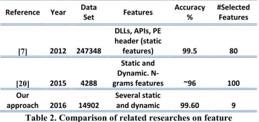
Reference Year Data_Set Features Accuracy_% #Selected_Features

[7] 2012 247348 DLLs, APIs, PE header (static features) 99.5 80 [20] 2015 4288 Static and Dynamic. N-grams features ~96 100 Our

approach 2016 14902 Several staticand dynamic 99.60 9

Table 2. Comparison of related researches on feature Selection and accuracy

2.4 Real-Time Malware Detection

Micha Moffie, Winnie Cheng and David Kaeli, 2006 [22] developed a security framework as complement to anti-virus programs called HTH. It is able to extract vast amount of runtime information in a “faster” manner (System calls, Library calls, Data flow), which is used for malware detection on real time. Regarding to this article, we believe that the overhead could be significant reduced if just the most important features are collected for detection on real time.

2.5 Problem Definition

As it is described, machine learning is not a new approach for malware detection and their accuracy is good compared to another type of data; however, given the huge traffic on internet and the exponential proliferation of malware, cyber security models require to be scalable, fast and flexible as stated by Ekta et al.[4]. With this in mind, one possible

(27)

improvement to current studies is to select the most representative features for malware detection in order to reduce the complexity of the models. Thus, having seen the Malware overview and related work, there are few studies related to selecting best features for Malware detection. As mentioned on previous sections, there are two current studies that performed feature selection but one of them just used static analysis (which is effective for obfuscation techniques – see reference [7]) and the other one, its accuracy is lower than the state of the art research – see reference[20]. In addition, it is a fact that models with thousand features requires long time for training and these are not suitable for real-time applications given that it requires intensive use of resources to extract the features during running time.

With this in mind, it is proposed the use of Machine Learning and Big Data tools for selecting the most representative features (from static and dynamic analysis) that keep the classification accuracy as high as of the state of the art models that use hundreds or thousands of features, allowing possible embedded programs to run fast looking for the characteristics that match malware behavior (it is important to mention that the creation of the embedded program is not the purpose of this thesis).

(28)

III. PROPOSED SOLUTION, IMPLEMENTATION AND RESULTS

In sum, the work presented on this research follows four main stages. First, the creation of a dataset by creating scripts-programs for downloading and parsing the metadata. Second, feature selection for reducing the datasets, removing noise and selecting the smallest number of features keeping accuracy high was accomplished.Next, training speed and accuracy improvement and finally, an additional work for adapting existing free tools for extracting the relevant behavioral and metadata features for malware detection is described on Appendix B.

3.1 The Dataset

In order to get the information from Malware and “good” files, it was considered two possibilities. First, use the Cuckoo Sand-box software [23], which is a platform for Malware analysis, for extracting information from programs executed on an isolated environment. In that way, a dataset of malware and “goodware” executable files was required, so malware dataset from Georgia Tech State University and a couple of others were downloaded. However, datasets of goodware files were harder to find and even more, the execution process of each file in an insulated environment and the extraction of information are so tedious, and time consuming, so a second option was evaluated.

The second option considered was to use VIRUSTOTAL[24], which is a free online service for analyzing files or URLs that runs a distributed setup of Cuckoo sandbox,

(29)

“enabling the identification of viruses, worms, Trojans and other kinds of malicious content detected by antivirus engines and website scanners”. In addition, VIRUSTOTAL provide information such as file version and properties, PE info, file metadata, and

behavioral information, so VIRUSTOTAL was chosen given that it is possible to save

the time regarding to the analysis because results are already available from the VIRUSTOTAL website. VIRUSTOTAL provide a public API for scanning, submit, and accessing to results. However, all the information is not public, so it was necessary to get the permission for having access to full scan results.

(30)

Figure 3. Sample of All-Info extracted from VirusTotal.

The first step to download the information from VIRUSTOTAL was to create a list of hashes for malware and “goodware” files. These two lists were created using the private API from VIRUSTOTAL and the query for malware hashes was any file with positive detection greater than 2 that belong to Windows OS. The query for “goodware” files was files with zero positives that belongs to NSRL and classified as “trusted” for Windows OS.

(31)

Next, using the same API and a couple of scripts, the lists of hashes were used to request the “behaviour” and the “allinfo” (see private API documentation for details). As a result, we got the information for 7630 malware files and 1818 “Goodware” scan reports (two json documents per each file containing the static, behavioral and metadata information).

Using R CRAN [25], the files were parsed and 57 different type of features were extracted; just for mentioned some ones, files opened, copied, deleted, etc, DLLs, codesize, Flags, datasize, language-code, file-info, entry-point, PE-info, imports, services, API-info, processes-info, network-info, among others. Finally, the information extracted was storage on matrices and the total number of features was 682.936 with a size of 22 GB. Finally, it is important to mention that for the current total population of malware, which is near to 600 millions of samples (according to statistics for August 2016 by AVTEST [3]), the sample size 9448 correspond approximately to a confidence level of 99% with a margin error of 1.33%.

The next two tables shows the number and type of features extracted from the JSON files “behavior” and “allinfo” per each submatrix created. For example, the matrix 29 on the table 3 contains 19128 features extracted from the “allinfo” json files that correspond to the “Imports”.

(32)

Features from "AllInfo" JSON file

# Number of Features Type of Features

1 43705 File System _ALL

2 2256 File System _COPIED

3 10767 File System _DELETED

4 1 File System _DOWNLOADED

5 8102 File System _MOVED

6 38525 File System _OPENED

7 8552 File System _READ

8 10 File System _REPLACED

9 17502 File System _WRITTEN

10 1394 Run Time DLLS

11 27 CHARACTERSET

12 1272 CODESIZE

13 14 FILE FLAGS MASK

14 10 FILE OS

15 4 FILE TYPE

16 3 FILE TYPE EXTENSION

17 1327 INITIAL DATA SIZE

18 52 Language Code

19 7 Object File Type

20 3 PE Type 21 7 SubSystem 22 178 Unpacker 23 4068 PE Entry Point 24 4 PE Machine Type 25 5108 PE Overlay Entropy

26 22 PE Overlay File Type

27 2433 PE Overlay Size

28 1446 PE Overlay Offset

29 19128 IMPORTS

30 323 SERVICES

31 97 TRID

(33)

Features from "behaviour" JSON file

# Number of Features Type of Feature

1 4024 SUMMARY FILES 2 164863 SUMMARY KEYS 3 2159 SUMMARY MUTEXES 4 50 CALLS API 5 12 CALLS CATEGORY 6 48353 CALLS RETURN 7 5 CALLS STATUS 8 67 CALLS ARGUMENTS_NAME 9 207222 CALLS ARGUMENTS_VALUE 10 13621 PROCESSES FIRST_SEEN 11 452 PROCESSES PARENT_ID 12 575 PROCESSES ID 13 9226 PROCESSES NAME

14 425 PPROCESS TREE PID

15 8466 PPROCESS TREE NAME

16 1620 NETWORK UDP_DPORT 17 818 NETWORK UDP_SPORT 18 2070 NETWORK UDP_DST 19 35019 NETWORK HOSTS 20 4168 NETWORK DNS_HOST 21 907 NETWORK HTTP_HOST 22 8161 NETWORK HTTP_URI 23 14 NETWORK HTTP_PORT 24 1506 NETWORK TCP_DPORT 25 1511 NETWORK TCP_SPORT 26 1275 NETWORK TCP_DST

Table 4. Type of "behavior" features per Matrix

3.2 Feature Selection

Feature selection is an important step for this research. As mentioned, one of the objectives is to select the smallest number of features that keep the detection rate as the state of the art models in order to minimize the resources for the malware detection task. Furthermore, feature selection and reduction is already know that can reduce the noise, improve the accuracy, and of course improve speed for training the classification algorithms as given that time increased in O(n2_{) with respect to the number of features as}

(34)

explained.

3.2.1 First Stage

Due to the large dimensionality, it was used SPARK given that this platform can deal with large datasets. The machine learning library for SPARK - MLlib – was used as first stage for feature selection. In particular, the Feature Selector “ChiSqSelector” was applied getting the 10 % of the most relevant features. This first reduced matrix contains 68.800 features with 9448 observations with a size of 2.2 GB. The use of “ChiSqSelector” is justified as a fast method for features selection for large datasets (it is not used in further steps as it might end up committing errors).

3.2.2 Second Stage

In this point, it was possible to select the best features running the Random Forest library (randomForest) on R–Cran (Rstudio) (ranking by decrease on accuracy and ranking on decrease on node impurity – see “importance” on randomForest package).

There are many algorithms for feature selection, which can be seen as techniques of combining features in subsets that are scored in order to determine relevant features. This search can be an intractable problem given the number of possible permutations. Furthermore, according to the metrics used these can be classified in three categories,

(35)

wrapper filter and embedded methods. In this research it is used the embedded methods for Random Forest by Mean Decrease in Accuracy and Mean Decrease in Impurity.

“Permutation Importance or Mean Decrease in Accuracy (MDA) is assessed for each feature by removing the association between that feature and the target. This is achieved by randomly permuting the values of the feature and measuring the resulting increase in error. The influence of the correlated features is also removed” and “Gini Importance or Mean Decrease in Impurity (MDI) calculates each feature importance as the sum over the number of splits (across all tress) that include the feature, proportionally to the number of samples it splits”[26].

In this process, six steps of reduction were developed running for each step the algorithms for classification. First, it was reduced from 68.800 features to 10.000 features, next to 5.000, 1.000, 300, 100, 31, 10 and finally 9 features.

3.3.3 Third Stage

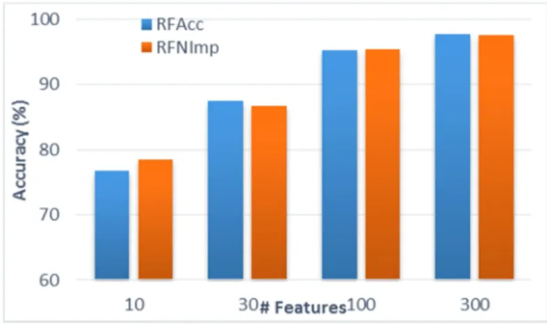
In order to validate how well the feature selection was being accomplished, classification algorithms as Support Vector Machine -SVM, Random Forest -RF and Artificial Neural Network -NN were used for tracking the classification accuracy. Figures Figure 4, Figure 5 and Figure 6 compare the accuracy as result of the described process.

(36)

Figure 4. Comparison on accuracy for the feature selection algorithms using Random Forest.

Figure 5. Comparison on accuracy for the feature selection algorithms using SVM.

(37)

From the charts above, it is possible to infer that ranking by decrease on accuracy (RFAcc) performs better than the other one. Furthermore, SVM classifier had a better behavior on accuracy than other methods specially using small amount of features. However, it is important to mention that Neural Networks were trained with just 100 iterations just for saving training time and because the objective in this stage was just compare the performance of the feature selection methods (no comparing the performance between classification algorithms).

Another important consideration to mention is that due to the unbalanced data (7630 malware files vs 1818 goodware files), oversampling was used (goodware files were duplicated 4 times, and thus the new amount of observations was 14902).

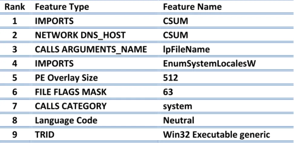
Next two tables show the main type of features to consider form malware detection and the selected best “9” features. (Note: CSUM correspond to the sum of the observation for each feature type, thus row 1 is the total number of “imports” that a specific program make).

Rank Feature Type Feature Name

1 IMPORTS CSUM

2 NETWORK DNS_HOST CSUM

3 CALLS ARGUMENTS_NAME lpFileName

4 IMPORTS EnumSystemLocalesW

5 PE Overlay Size 512

6 FILE FLAGS MASK 63

7 CALLS CATEGORY system

8 Language Code Neutral

9 TRID Win32 Executable generic

(38)

Feature Type 100 Features Dataset 30 Features Dataset # Features % # Features % CALLS ARGUMENTS_VALUE 20 20.0 2 6.5 IMPORTS 19 19.0 6 19.4 TRID 10 10.0 6 19.4 CALLS ARGUMENTS_NAME 9 9.0 1 3.2 CALLS RETURN 8 8.0 2 6.5 NETWORK UDP_DST 4 4.0 1 3.2 Language Code 4 4.0 1 3.2 NETWORK HOSTS 3 3.0 1 3.2 CALLS API 2 2.0 1 3.2 CALLS CATEGORY 2 2.0 1 3.2 NETWORK UDP_DPORT 2 2.0 0 0.0 NETWORK UDP_SPORT 2 2.0 0 0.0 NETWORK DNS_HOST 2 2.0 1 3.2 NETWORK TCP_DPORT 2 2.0 1 3.2 Run Time DLLS 2 2.0 2 6.5 PE OVERLAY SIZE 2 2.0 1 3.2 SUMMARY MUTEXES 1 1.0 0 0.0 NETWORK TCP_SPORT 1 1.0 1 3.2 NETWORK TCP_DST 1 1.0 1 3.2 FILE FLAGS MASK 1 1.0 1 3.2 FILE OS 1 1.0 1 3.2 UNPACKER 1 1.0 0 0.0

Table 6. Feature Type Importance

3.3 Results of Classification Algorithms

In this section, accuracy performance for Random Forest and Neural Networks are tested with different number of features. Next, Support Vector Machine is used to preprocess feature vectors as a previous step to apply Neural Networks. Finally an assembly model is build and tested for the current dataset and a newer dataset from previously unknown malware files.

(39)

3.3.1 Preliminary Accuracy Results

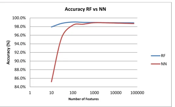
In this first stage, three main algorithms were used, Random Forest (RF), Support Vector Machine (SVM) and Neural Network (NN) in R-Cran (packages “randomForest” and “nnet”). To mention, the whole dataset was divided in training dataset and testing dataset. The testing set was 3724 observations that correspond to the 25% of the original “balanced” dataset.

Results showed that Random Forest (RF) presented similar accuracy to Neural Network (NN) for large number of features; however SVM was better in general, especially for smaller number of features. Regarding to the parameters for RF, the number of trees to “grow” was 1000. For NN, the number of iterations was 200 (other parameters as default). It’s important to mention that RF had a better True Positive Rate than NN, which implies RF had better performance to classify “goodware” samples.

In addition, NN had a lower False Positive Rate than RF, so NN classify better the “malware” samples, but compared to SVM, this last one had a better performance at all. Finally, regarding to accuracy, SVM presented a peak in accuracy around 9 and keep almost the same (in fact decrease) even when the features increase. Note: Positive refers to “Goodware” (P).

(40)

Figure 7. Accuracy for RF and NN through the number of features.

Figure 8. Accuracy for SVM through the number of features.

3.3.2 Improving Neural Network classification performance

On this stage, it was first decided to work in deep on the Neural Network, given that previously It was just used 200 iterations. The neural network model used was the NN package on TORCH with one hidden, one Tanh and one logsoftmax layer. Also, we divided the dataset on 70% for Training and 30% for Testing (Note that previously it was divided 75% - 25%, so in general accuracy results in testing dataset decreased). Using the

84.0% 86.0% 88.0% 90.0% 92.0% 94.0% 96.0% 98.0% 100.0% 1 10 100 1000 10000 100000 Ac cu rac y (% ) Number of Features Accuracy RF vs NN RF NN 75 80 85 90 95 100 0 5 10 15 20 25 30 Ac cu rac y (% ) # Features

(41)

dataset with the best 30 features selected by RF-decrease on accuracy, and running the NN, results showed that even with a large number of iterations, the accuracy does not increased considerably.

Figure 9. Test Accuracy for best 30 features dataset.

Here is interesting to ask why SVM has better performance in this case. Without going deep, simple Neural Networks (with one or some small hidden layers) are based on combinations of sums of their inputs multiplied by weights and some nonlinear functions as tanh or sigmoid or RELU applied on particular layers. On the other hand, SVM uses nonlinear kernels (polynomial, radial basis functions, tanh) to transform its inputs into a hyperplane that is easier to separate. Thus, we could think that using the power of transforming the feature vectors one by one to an easier separable hyperplane and then to allow NN to build separation spaces for whole transformed dataset could be a good idea.

Further, we introduce simples but effective steps to preprocess the dataset to improve not just the training speed but also the accuracy of the Neural Network algorithm. First,

0.86 0.8650.87 0.8750.88 0.8850.89 0.895 1 10 100 1000 # Iterations Test Accuracy

(42)

Being said that, we applied SVM oneach feature vector.

Thus, after having tried the polynomials and Radial base functions, this last one presented the best results for transform each feature vector into a hyperspace. After having applied these transformations with the SVM, we assembled all of these new feature vectors into another dataset and the Neural Network was trained again.

Next charts compare the behavior of the training error – Err (the track of the errors or loss during the training process) and the accuracy – Acc (gotten on the test dataset for each iteration) for the Neural Network applied to the original dataset – Base-, and the NN applied to the transformed dataset –withSVM.

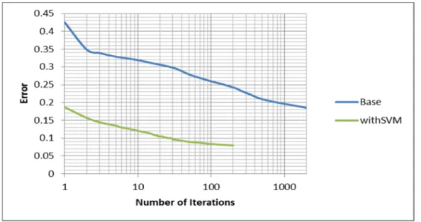
Figure 10. Comparison of Training Errors for best 30 features dataset (75% training – 25% test) (Base dataset and transformed with SVM).

(43)

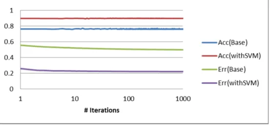
Figure 11. Comparison of Training Errors (Err) and Test Accuracy (Acc) for best 30 features dataset (Base dataset and transformed with SVM. 70% training – 30% test).

Figure 12. Comparison of Training Errors and Test Accuracy for best 9 features dataset (Base dataset and transformed with SVM70% training – 30% test).

From Figure 10 we can see that the training error after 2000 iterations on the base dataset is reached with just two iterations on the transformed dataset and it is also the double of the error after 200 iterations on the transformed dataset. Even more, from Figure 11 and Figure 12, the accuracy from the test dataset increased around 8% to 17% and errors decreased around 55% to 60% in average. In fact just with one iteration, results are better that the base dataset after 2000 iterations (see Figure 11) or 1000 (see Figure 12) iterations.

(44)

preprocessing discussed is transforming the feature vectors applying functions to transform to another space easier separable. Even more, we can apply other classification algorithms to each feature and get a dataset that is easier to classify. Next, we show a brief explanation sample.

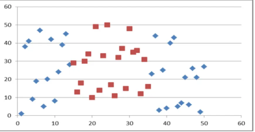
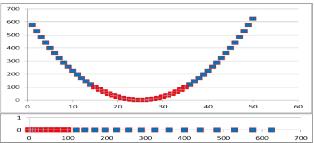
Suppose you have the dataset in the Figure 13. Next you can take each feature vector by separate as shown in Figure 14. If you apply a quadratic function to the data on Figure 155 and a sinusoidal function to Figure 166, you can transform the original dataset into an easier separable space as shows in Figure 177.

Figure 13. Original sample dataset.

(45)

Figure 15. Quadratic function applied to feature vector one.

Figure 16. Sinusoidal function applied to feature vector two.

(46)

Forest just for illustrating how it looks like.

Figure 18. Three feature vectors from the original dataset.

(47)

In sum, the preprocessing discussed is transforming the feature vectors applying functions to transform to another space easier separable. Concluding this section, preprocessing the feature vectors by separated before training the classification algorithms increase the accuracy and the speed given that with few iterations is possible to get lower errors and better accuracy (at least it was valid on our dataset using the Neural Network algorithm). It is also important to mention that the time to transform the features, let say of our 30 best feature dataset, it was around six minutes, which compared with the time that took to train the NN with this dataset (around a couple of hours or more) is small. Note: SVM was also applied after transform the feature vectors with the SVM, but the accuracy remains quite similar and sometimes it decreased.

3.3.3 Improving the Test Accuracy on the Best 9 Features Dataset:

In this section we present the process used for improving the current Test Classification Accuracy, which is 99.2% for the 9 best features using the SVM algorithm. (SVM was used to track the accuracy sequentially adding feature vectors in the ranked order. We saw that with the first 9 features the higher accuracy is reached).

At this point, it was decided to create a new dataset from combining The original best 9 features dataset plus its transformed one applying SVM and RF to each feature vector, plus the dataset after PCA transformation, the results by RF from the original dataset, the results by RF from the dataset transformed by PCA and the results by SVM to the original dataset.

(48)

show that SVM made overfitting and the accuracy decreased on the testing dataset. However, NN shows a significant improvement, achieving an accuracy results near to 99.4%. Consequently, we decided to use the schema shows on the Figure 20, where we tried different combinations to create a new dataset that give us the best result.

Finally after around 40 combinations, we found that the schema on Figure 21 gives the best result, which increase the Testing Accuracy up to 99.6% from the best 9 features. This schema includes the original dataset, the transformed dataset by SVM applied to each feature and the results by SVM applied to the original dataset.

Note: The total time required for create the dataset and training the schema on Figure 21 was around 16 minutes, and the NN required 255 iterations -13 minutes, to reach the maximum accuracy value.

 The configuration of the NN was as follow:

Package TORCH “nn”

sgd_params = {learningRate = 2e-2, learningRateDecay = 1e-4, weightDecay = 1e-3, momentum = 1e-4} net = nn.Sequential() net:add(nn.Linear(19, 10)) net:add(nn.Dropout(0.2)) net:add(nn.Linear(10, 4)) net:add(nn.ReLU()) net:add(nn.Linear(4, 2)) net:add(nn.LogSoftMax()) criterion = nn.ClassNLLCriterion()

(49)

Note 1: Simulations were performed on a server with the next specifications:

 Processor: Intel Core i7-3930k CPU @ 3.20 GHz x12

 Graphics Tesla C2075/PCIe/SSE2

 OS Type 64-bit

 RAM 48 GB

 OS UBUNTU 14.04 LTS

(50)

Figure 21. Best assembly classification schema

Finally, we decided to build the Receiver Operating Characteristic – ROC curve, which shows great performance for our classifier (the area under the curve - AUC was around 0.997). Next, the ROC curve is shown on the Figure 22.

(51)

3.3.4 Verifying the robustness of the model

In this section, the model is intended to be tested on malware files that belong to Zero Day Attacks, which would show the robustness of the model to detect malware that exploit unknown vulnerabilities on software products. In addition, a new dataset of malware files classified as seen by first time on dates posteriors to the creation of the original dataset was created and tested with the model, thus the robustness of our model to detect new samples of malware is checked.

3.3.4.1 Zero Day Vulnerabilities:

What is Zero Day Vulnerability and attack? According to [27] and [28], Zero Day Vulnerabilities refers to a hole that is unknown to the vendor and can be exploited by hackers to affect adversely computers, networks, data, etc. The term “zero day” refers to the unknown nature of the hole to the developers, but once the vulnerability becomes known, developers need to release patches to mitigate the damage.

Zero-day protection is the ability to provide protection against zero-day exploits, which is often difficult given the nature of the unknown treat. For example, “Zero-day attacks are often effective against "secure" networks and can remain undetected even after they are launched”[28].

In order to determine the robustness of our model to detect Zero Day Attacks, a list of 480 vulnerabilities from years 2015 and 2016 was created from [29]. Next, using

(52)

vulnerabilities. In this way, we got a list of 297 hashes of malware related to Zero Day Attacks. The Next step was download the behavioral information extracted by VirusTotal, and the result was 3 JSON files with not empty information (294 hashes belongs to malware which behavioral information is empty). Given that 3 zero-day malware files are not enough to test our model with statistical consistency, it was decided to avoid test the model with this data, so it is not possible conclude the effectiveness of the model to detect Zero Day Attacks. In addition, a point to consider is the amount of empty behavioral files from VIRUSTOTAL regarding to this zero-day attacks, clearly requires further research.

Figure 23. Zero Day Attach hash sample 1.

(53)

Figure 25. Zero Day Attach hash sample 3.

3.3.4.2 New Malware Dataset:

This new dataset of malware files was gotten searching by the hashes of malware files of malware seen by first time between November 2015 to June 2016. The dataset contains 253 malware files and the testing results for our model was 98,4% of “accuracy”, which in this case correspond to the True Negative Rate TNR given that the dataset contains just malware samples. In sum, we can see that the model, which was trained with samples previous to October 2015, is able to classify new unseen malware files with an acceptable good accuracy.

(54)

IV. CONCLUSIONS

Reaching the final step of this research many lessons were learned not only regarding to the security point of view but also from machine learning topics. Initially, it was seen that there are absence of “goodware” and malware datasets that researches can use to compare results. However, great tools as Virustotal can be used to download many behavioral and metadata information.

Regarding to the objectives of this thesis, feature selection showed that it is possible to use few features to reach high level of accuracy for malware detection, which could implies to reduce resources in programs that look for detecting malware, and warn software developers to study further how these important features could be related to security breaches. Thus, the best classification accuracy can be gotten using the 9 features ranked by Random forest by decrease on accuracy.

In addition, SVM algorithm showed a great performance compared to RF and NN; however combining algorithms can lead to better results at it happened in our case. Final accuracy results with the assembly structure proposed was 99.6%, which is even better than classifications without feature selection with hundreds or thousands of features. In terms of numbers, our results showed that assuming a simple sample size of 7630 malware files from a population of 600 Millions, we could say that we were 99% sure that our model could detect a malware between 99.2% +/- 1.5% using just 9 features.

(55)

An important finding to mention was that transforming the dataset by applying SVM to each feature vector could lead to increase accuracy and performance for further use of classification algorithms applied to the whole dataset (at least it was valid on our dataset using the SVM or RF for preprocessing each feature vector by separated and then using Neural Network or RF algorithms for classification). Furthermore, the vector feature transformation opens the possibility to explore building new architecture layers on the Neural Network; we believe that structures that allows emulate more complex functions as polynomials, exponentiation, etc. on the NN could help to increase the overall performance.

As a final suggestion for researches, further analysis is required to select best features that can be extracted in a faster manner; it would help to build a light weight embedded program for monitoring suspicious behavior.

(56)

V. REFERENCES

[1].Xin Hu, “Large-Scale Malware Analysis, Detection, and Signature Generation,” The University of Michigan, 2011.

[2].Igor Santos, Jaime Devesa, Felix Brezo, Javier Nieves, and Pablo G. Bringas, “OPEM: A Static-Dynamic Approach for Machine-learning-based Malware Detection,” Deusto Institute of Technology University of Deusto, Bilbao, Spain. Year: 2013.

[3].AVTEST. March 2017. “Malware”. Retrieved from https://www.av-test.org/en/statistics/malware/

[4].Ekta Gandotra, Divya Bansal, and Sanjeev Sofat, “Malware Analysis and Classification: A Survey,” IPEC University of Technology, Chandigarh, India. Journal of Information Security. April 2014.

[5].Cloud Security Alliance, “Expanded Top Ten Big Data Security and Privacy Challenges,” April, 2013.

[6].J. Zico Kolter, and Marcus A. Maloof, “Learning to Detect and Classify Malicious Executables in the Wild,” Stanford University. Journal of Machine Learning Research 7. 2006.

[7].Usukhbayar Baldangombo, Nyamjav Jambaljav, and Shi-Jinn Horng, “A Static Malware Detection System Using Data Mining Methods,” National University of Mongolia, and University of Science and Technology, Taipei, Taiwan. 2012.

[8].D. Swathigavaishnave, and R. Sarala, “Detection of Malicious Code-Injection Attack Using Two Phase Analysis Technique,” Pondicherry Engineering College Puducherry, India. May 2012.

[9].Schultz, M., Eskin, E., Zadok, F. and Stolfo, S. (2001) Data Mining Methods for Detection of New Malicious Executables. Proceedings of 2001 IEEE Symposium on Security and Privacy, Oakland, 14-16 May 2001, 38-49. [10]. Kolter, J. and Maloof, M. (2004) Learning to Detect Malicious

Executables in the Wild. Proceedings of the 10th ACM. SIGKDD

International Conference on Knowledge Discovery and Data Mining, 470-478.

[11]. Nataraj, L., Karthikeyan, S., Jacob, G. and Manjunath, B. (2011) Malware Images: Visualization and Automatic Classification. Proceedings of the 8th International Symposium on Visualization for Cyber Security, Article No. 4. [12]. Rieck, K., Trinius, P., Willems, C. and Holz, T. (2011) Automatic

Analysis of Malware Behavior Using Machine. Learning. Journal of Computer Security, 19, 639-668.

(57)

[13]. Anderson, B., Quist, D., Neil, J., Storlie, C. and Lane, T. (2011) Graph Based Malware Detection Using Dynamic. Analysis. Journal in Computer Virology, 7, 247-258. http://dx.doi.org/10.1007/s11416-011-0152-x

[14]. Firdausi, I., Lim, C. and Erwin, Analysis of Machine Learning Techniques Used in Behavior Based Malware Detection, Proceedings of 2nd

International Conference on Advances in Computing, Control and Telecommunication Technologies (ACT), Jakarta, 2010, 201-203. 2010 [15]. Rafiqui Islam (Charles Sturt University, NSW 2640, Australia), Ronghua

Tian (Deakin University, Victoria 3125, Australia), Lynn M. Battena and, Steve Versteeg (CA Labs, Melbourne, Australia), “Classification of malware based on integrated static and dynamic features,” Journal of Network and Computer Applications 36 (2013) 646–656. 2013.

[16]. Anderson, B., Storlie, C. and Lane, T. (2012) Improving Malware Classification: Bridging the Static/Dynamic Gap. Proceedings of 5th ACM Workshop on Security and Artificial Intelligence (AISec), 3-14.

[17]. Michal Kruczkowoski (Research and Academic Computer Network NASK, Warsaw, Poland) and Ewa Niewiadomska (Institute of Control and Computation Engineering, Warsaw University of Technology, Warsaw, Poland), “Comparative Study of Supervised Learning Methods for Malware Analysis”. 2014

[18]. Ohm Sornil (National Institute of Development Administration, Bangkok, Thailand), and Chatchai Liangboonprakong (Suan Sunandha Rajabhat University, Bangkok, Thailand), “Malware Classification Using N-grams Sequential Pattern Features,” International Journal of Information Processing and Management (IJIPM) Volume4, Number5. July 2013.

[19]. Mariano Grazing, Davide Canali and Davide Balzarotti (Eurecom), Leyla Bilge (Symantec Research Labs), Andrea Lanzi (Universita’ degli Studi di Milano), “Needles in a Haystack: Mining Information from Public Dynamic Analysis Sandboxes for Malware Intelligence,”. 2015.

[20]. Chih-Ta Lin, Nai-Jian Wang, Han Xiao and Claudia Eckert. “Feature Selection and Extraction for Malware Classification”. National Taiwan University of Science and Technology, Taipei. Taiwan. 2015.

[21]. George E. Dahl (University of Toronto, Toronto, ON, Canada), and Jack W. Stokes, Li Deng, Dong Yu (Microsoft Research, One Microsoft Way Redmond, WA 98052, USA), “Large-Scale Malware Classification Using Random Projections And Neural Networks,” ICASSP. 2013.

[22]. Micha Moffie, avid Kaeli (Northeastern University, Boston, MA) and Winnie Cheng (Massachusetts Institute of Technology Cambridge, MA), “Hunting Trojan Horses”. 2006.

[23]. Cuckoo-Sandbox. http://www.cuckoosandbox.org/

[24]. VirusTotal - Free Online Virus, Malware and URL Scanner. https://www.virustotal.com/en

(58)

Retrieved from http://alexperrier.github.io/jekyll/update/2015/08/27/feature-importance-random-forests-gini-accuracy.html

[27]. PCTOOLS by Symantec. Security news. Retrieved from http://www.pctools.com/security-news/zero-day-vulnerability/

[28]. Wikipedia, March 27, 2017. Zero-day (Computing). Retrieved from https://en.wikipedia.org/wiki/Zero-day_%28computing%29.

[29]. CVE Common Vulnerabilities and Exposures. March 2017. Retrieved from https://cve.mitre.org/

[30]. PE File. Retrieved from

http://repo.hackerzvoice.net/depot_madchat/vxdevl/papers/winsys/pefile/pefi le.htm

[31]. Matt Pietrek. March 1994. Microsoft Documentation. “Peering Inside the PE”. Retrieved from

https://msdn.microsoft.com/en-us/library/ms809762.aspx

[32]. Mario Vuksan and Tomislav Pericin. Reversing Labs. 2011. “Constant insecurity”. Retrieved from

https://media.blackhat.com/bh-us-11/Vuksan/BH_US_11_VuksanPericin_PECOFF_Slides.pdf

[33]. Wikipedia. January 2017. “Dynamic-link Library”. Retrieved from https://en.wikipedia.org/wiki/Dynamic-link_library

[34]. Microsoft. “Windows API sets”. Retrieved from

https://msdn.microsoft.com/en-us/library/windows/desktop/hh802935%28v=vs.85%29.aspx [35]. Wikipedia. March 17. “Windows API”. Retrieved from

https://en.wikipedia.org/wiki/Windows_API

[36]. Jacquelin Potier. “WinAPIOverride”. Retrieved from

http://jacquelin.potier.free.fr/winapioverride32/documentation.php [37]. Phil Harvey. March 2017 “ExifTool”. Retrieved from

http://www.sno.phy.queensu.ca/~phil/exiftool/

[38]. Cuckoo-Modified. GitHub. November 2015. Retrieved from https://github.com/brad-accuvant/cuckoo-modified/tree/master/docs [39]. Ascend4nt. August 3, 2013. “PE Overlay Extraction”. Retrieved from

https://www.autoitscript.com/forum/topic/153277-pe-file-overlay-extraction/ [40]. Marco Pontello. March 2017. “TrID – File Identifier”. Retrieved from

http://mark0.net/soft-trid-e.html

[41]. Windump. Retrieved from https://www.winpcap.org/windump/

[42]. Smita Ranveer, and Swapnaja Hiray, “Comparative Analysis of Feature Extraction Methods of Malware Detection,” Sinhgad College of Engineering, Savitribai Phule Pune University, India. International Journal of Computer Applications (0975 8887) Volume 120 - No. 5. June 2015. [43]. Wikibooks. February 2, 2017. “x86 Disassembly”. Retrieved from

https://en.wikibooks.org/wiki/X86_Disassembly/Windows_Executable_Files [44]. Ero Carrera. December 2016. “pefile”. Retrieved from

(59)

[45]. Microsoft. “Windows Sysinternals. Process Monitor v3.32”. Retrieved from https://technet.microsoft.com/en-us/sysinternals/processmonitor.aspx [46]. Rohitab Batra. 2012. “API Monitor”. Retrieved from

http://www.rohitab.com/apimonitor

[47]. Margaret Rouse. 2005. “Elk Cloner”. Retrieved from http://searchsecurity.techtarget.com/definition/Elk-Cloner

(60)

APPENDIX A: SOFTWARE IMPLEMENTATION FOR MALWARE

DETECTION

As referenced on table 5 and restated on next table, the selected best “9” features are as follow.

Rank Feature Type Feature Name

1 IMPORTS CSUM

2 NETWORK DNS_HOST CSUM

3 CALLS ARGUMENTS_NAME lpFileName

4 IMPORTS EnumSystemLocalesW

5 PE Overlay Size 512

6 FILE FLAGS MASK 63

7 CALLS CATEGORY system

8 Language Code Neutral

9 TRID Win32 Executable generic

In this additional section, it is presented information regarding the different type of data that need to be extracted from files for the malware detection purpose. This information will give the general idea about where come from the data and why it is important for malware detection. Finally, it is described how doing modifications to existing free tools, it is possible to create an embedded program to monitor relevant features for malware detection.

A.1 Portable Executable File Format (Pe):

The "portable executable file format" (PE) specify the structure of the binary executable programs (exe, dll, sys, scr) and object files (bpl, dpl, cpl, ocx, acm, ax) for MS windows NT, windows 95 and win32s[30].

(61)

The format was designed by Microsoft as a standard for Microsoft, Intel, Borland, Watcom, IBM and others, that share "common object file format" (COFF - the format used for object files and executables on several UNIX and VMS Oses)[30].

Loading an executable into memory is requires to map structures from the PE file into the address space, therefore the information on memory will have almost the same structure of PE files. The information mapped into memory represents all the code, data, and resources that a program requires to be executed. However some parts of a PE file may be read, but not mapped, for example, when debug information is placed at the end of the file. In the case of Windows, the “Win32 loader” decides what portions of the file to map in memory.

In general, the structure of a PE file follow the next pattern, a DOS MZ Header, DOS Stub, PE File Header, Optional Header, Section Table, and Sections. Here it is important to mention that this structure could be changed; in fact some malware is created altering this structure.

Each section header has some flags about what kind of data it contains ("initialized data"," readable data","writable data", etc), and pointers. A PE header component is called the "IMAGE_DIRECTORY HEADER". This header holds information about some PE Sections (Resources, Import, and so on). Each Record being [PointerToSection] [Size].