Risk Transfer with CDOs and Systemic Risk in Banking

No. 2006/04

Risk Transfer with CDOs and Systemic Risk in

Banking

Center for Financial Studies

The

Center for Financial Studies

is a nonprofit research organization, supported by an

association of more than 120 banks, insurance companies, industrial corporations and

public institutions. Established in 1968 and closely affiliated with the University of

Frankfurt, it provides a strong link between the financial community and academia.

The CFS Working Paper Series presents the result of scientific research on selected

topics in the field of money, banking and finance. The authors were either participants

in the Center´s Research Fellow Program or members of one of the Center´s Research

Projects.

If you would like to know more about the

Center for Financial Studies

, please let us

know of your interest.

* _{We are grateful for financial support by Deutsche Forschungsgemeinschaft (DFG) and by Frankfurt University’s Center for Financial}

Studies (CFS). This paper is part of CFS’ project on the Economics of Credit Risk Transfer. In developing the basic question of this paper, we owe a lot to mini workshops with Günter Franke as well as Dennis Hänsel and Thomas Weber. We also thank seminar participants at the 2005 Meeting of the German Finance Association in Augsburg and the 2005 Annual meeting of the Verein für Socialpolitik in Bonn.

1 _{Finance Department, Goethe-University, Center for Financial Studies (CFS), Frankfurt, and CEPR.}

Correspondence: CFS, Mertonstraße 17-21, 60325 Frankfurt(Main), Germany, Email: [email protected]

CFS Working Paper No. 2006/04

Risk Transfer with CDOs and

Systemic Risk in Banking*

Jan Pieter Krahnen

and Christian Wilde

March 1, 2006

Abstract:

Large banks often sell part of their loan portfolio in the form of collateralized debt obligations

(CDO) to investors. In this paper we raise the question whether credit asset securitization

affects the cyclicality (or commonality) of bank equity values. The commonality of bank

equity values reflects a major component of systemic risks in the banking market, caused by

correlated defaults of loans in the banks’ loan books.

Our simulations take into account the major stylized fact of CDO transactions, the

non-proportional nature of risk sharing that goes along with tranching. We provide a theoretical

framework for the risk transfer through securitization that builds on a macro risk factor and an

idiosyncratic risk factor, allowing an identification of the types of risk that the individual

tranche holders bear. This allows conclusions about the risk positions of issuing banks after

risk transfer.

Building on the strict subordination of tranches, we first evaluate the correlation properties

both within and across risk classes. We then determine the effect of securitization on the

systematic risk of all tranches, and derive its effect on the issuing bank’s equity beta. The

simulation results show that under plausible assumptions concerning bank reinvestment

behaviour and capital structure choice, the issuing intermediary’s systematic risk tends to rise.

We discuss the implications of our findings for financial stability supervision.

JEL Classification:

G28

1

Introduction

Securitization of loan assets has become a common instrument of bank risk man-agement. According to [10], a survey published by the European Central Bank in 2004, about 8-15% of overall assets of large, international banks, have been subject to a securitization transaction. Many observers, such as J.P. Morgan (2004), believe the market for asset backed securities (ABS) to grow rapidly in the next couple of years. What is the impact of securitizations on the risk exposure of the issuing institutions? In particular, how are commercial banks

affected that hold large volumes of loans on their balance sheets and that engage

in securitizing them?

The answers to these questions are not obvious at all. According to Green-baum and Thakor (1987), credit securitization allows a bank to reduce its risk

exposure, and to increase diversification in the economy. In the model of Duffie

and Gârleanu (2001), securitizations improve liquidity and induce a positive

overall market value effect. However, the effective risk transfer from a bank’s

balance sheet is limited by moral hazard problems. Allen and Gale (2004) ar-gue that, for incomplete markets, credit risk transfer may in fact increase risk

concentration rather than risk diversification, thereby raising overall systemic

risk. While risk transfer has often been cited as a major driver of ABS market development, we will show below that in a typical CLO and CDO transaction (i.e. collateralized loan obligations, collateralized debt obligations), risk transfer is rather limited, irrespective of the impressive size of the issues. The key to understanding risk transfer in structured transactions, such as ABS and CDOs, lies in the non-proportional sharing of risk. The tranching of claims, and the

application of the subordination principle, lead to a reshuffling of risk in the

portfolio. Typically, tail risk is being transfered, while non-tail risk is retained by the issuing bank. This is particularly true for asset pools that are subject

to moral hazard, such that retention of the most junior tranche, thefirst loss

piece, serves as a bonding and signaling device (DeMarzo, 2005). Tranching and securitization therefore alters, or may alter, three aspects of the issuer’s

risk position. First, it truncates the loss rate distribution. Second, it affects

the correlation between on-balance sheet assets and, third, it may change the systematic risk of the company, its exposure against market-wide risk factors.

In this paper we address all three consequences of asset securitization. We model a bank that repeatedly securitizes its loan portfolio, while retaining the

first loss piece, and that reinvests the proceeds by lending to customers. Given

the risk characteristics of the loan portfolio, how does securitization change the basic properties of the bank’s remaining loan book, i.e. its loss rate distribution? what are the correlations between the retained asset portions and the remaining asset on the balance sheet? Furthermore, how can the risks be characterized

that are transfered offthe balance sheet, and on to the buyers’ books? Are they

mostly systematic or rather company-specific, i.e. of an unsystematic nature?

Finally, how is the dependence of bank equity values on a macroeconomic factor

affected, does it increase or decrease?

with Das et al. (2004), investors will price structured finance products, like senior or mezzanine tranches of a CDO transaction, by looking at the amount of systematic default risk that they carry. For this purpose, systematic default risk has to be estimated. For regulators, risk shifting between banks and capital

markets is relevant since it may affect the required capital base of individual

banks and, even more importantly, it may affect the exposure of the banking

system at large vis-à-vis macroeconomic risks, see Andersen et al. (2004). The analysis relies on a two-stage procedure: First, the loss distribution of the underlying portfolio has to be determined. Subsequently, the loss

distribu-tion is allocated to tranches, representing claims of different seniority on the

underlying portfolio. We apply a Monte Carlo simulation to model the loss

distributions for portfolios of bank loans. For tranching, we apply cut-offvalues

represented by maximum default probabilities allowed for each tranche. In prac-tice, these values are indicated by rating agencies. The data are then used to

describe the correlation property between tranches of different seniority and/or

different underlying asset pools. Our asset value model allows to disentangle the

effects of an economy-wide risk factor from risks associated with an industry, or

a particular company.

The results show that, among tranches of different transactions with the

same credit quality (intra-rating correlations), the most senior tranches have

the highest correlation coefficient.

Second, the correlation between tranche performance and the realization of the macro factor is monotonically related to the degree of subordination. In particular, senior tranches have a low systematic risk, while junior tranches show high systematic risk.

These findings allow to asses the effect of securitizations on the systematic

risk of bank equity and, ultimately, on the systemic risk of the banking industry as a whole. We argue that, as the banks apply themselves to the securitization of individual loan books, they will most likely increase their systemic expo-sure, rather than reduce it. This, in turn, will contribute to an increase in the probability of banking crises.

The paper is structured as follows: First, we describe how CDOs can be

modeled. We present the model setup, based on afirm-value model, and

dis-cuss the implementation based on Monte Carlo simulation. Second, we look at a single transaction and investigate which risks are transfered from the underlying loan portfolio to tranches as part of securitization. Third, we turn to the level of individual institutions. We infer the consequences of securitization for the

risk positions of typical banks and examine the benefits of loan portfolio

diver-sification in the context of securitization. We also derive how bank equity betas

change after banks securitize their loan portfolios. Fourth, at the level of the overall economy, we examine the interaction of banks and the consequences of securitization for systemic risk. In the concluding section we discuss the

2

Modeling CDOs

In this section we will analyze the risk charactristics of asset backed securities

and relatedfinancial instruments1_{. We construct a simple tool that allows us}

to portray the loss distribution of asset portfolios, and of any tranche that is derived from the same underlying portfolio.

2.1

Model setup

We apply afirm-value model to capture the occurrence of obligor default. More

precisely, we apply a structural one-factor correlated default model. The driving factor is a market factor, and company value is modeled as the interplay of the

market factor and a company specific, idiosyncratic risk factor. This market

model approach is the model of choice in most corporate finance applications.

We model company value Vn,t of each obligor n ∈ {1,2, ..., N} at any time

t before maturity as being driven by a generalized macroeconomic factor YM

t

that is common to all securities, and an idiosyncratic component n,t:

Vn,t= q ρM n YtM + q 1₋ρM n n,t (1) with YM

t ∼ Φ(0,1), and n,t ∼ Φ(0,1). Thereby, we obtain correlated

asset values of obligors. In case the sensitivities pρM

n of firm values to the

macroeconomic risk factor are the same for all obligorsn, thenρM

n corresponds

to the mutual correlation coefficient for all assets.2

Obligor nis assumed to default if at any timet the valueVn,t of its assets

lies below the exogenously given default boundaryDn, i.e. Vn,t< Dn. Vn,t is

assumed to be normally distributed and is standardized such thatVn,t ∼Φ(0,1).

There is a simple relation linking every default boundaryDnto a particular

default probabilitypn:

Dn=Φ−1(pn). (2)

1_{Asset backed securities are structuredfinancial instruments that share two basic features:}

the pooling of underlyingfinancial claims, and their tranching into a set of bonds, differentiated by the degree of subordination. See Jorion or Fabozzi for institutional details.

2_{A more general model setup allowing for both inter- and intra-industry correlation}

could include, besides the market factor, orthogonal industry factors Y_tj for industries

j ∈ {1,2, ..., J}. The company value of each obligor in industry j can be modeled as:

Vn,tj = p ρM nYtM + q ρjnYtj+ q 1−ρM n −ρ j n n,t, withYtM ∼Φ(0,1), Y j t ∼Φ(0,1), and t

n∼Φ(0,1). We assume that securities within industries are driven by a factorY j t that is

orthogonal toYM

t and specific for that particular industry, i.e. Cov

³ Yi t, Y j t ´ = 0fori6=j. Thereby, we obtain correlated asset values of obligors within the same industry, with corre-lation coefficientρjnfor industryj. The chosen representation also allows for inter-industry

correlations, captured by ρM

n. This approach is quite general and accounts both for both

inter- and intra-industry correlations. Its structure encompasses the approaches commonly applied by major rating agencies, which rely on a one factor model for each industry and zero inter-industry correlation. Thus, it reduces to the classical market model if industry-specific risk is zero, while it reduces to the agency model if only the industry-specific component has explanatory power.

Usually, a fraction of the notional amount can be recovered in case of default.

Letψ_ndenote the recovery rate andθnthe exposure size of securityn. Portfolio

loss is given as the sum of individual loan losses. We define the portfolio default

rateP DRas the present value of portfolio loss divided by the net present value

of all promised payments until maturity:

P DR= PN n=11{Tn>τn}·θn· ¡ Fn·(1−ψn)·e−rτn+Cn,τn,Tn·e− rTn¢ PN n=1θn·(Fn+Cn,0,Tn)·e−rTn , (3)

where 1_{Tn>τn} is an indicator function taking the value one if security

n defaults during its lifetime and zero otherwise. Tn represents maturity of

security n, and τn is the time of default. Fn denotes the redemption value

andCn,sn,tn represents the present value at timetn of all coupon payments for

security n paid in the time interval [sn, tn]. All payoffs are discounted with

interest rater.

The appliedfirm value model (Eq. 1) is suitable for a simulation exercise.

2.2

Model implementation

In the implementation, we do not need to apply simplifying assumptions to de-termine the loss distribution of the underlying portfolio. Instead, we are able to

fully profit from the Monte Carlo Simulation procedure. Analytical approaches

often rely on limiting assumptions, e.g. that the portfolio is composed of an infi

-nite number of securities with identical characteristics. Thus, analytical models to some extent may be suitable for sensitivity analyses, but Monte Carlo Simu-lation is more appropriate for real-world applications. All individual securities

in the portfolio can be accounted for by their specific exposure size, recovery

rate, default probability, and maturity. Furthermore, Monte Carlo Simulation

allows to differentiate between obligors and individual securities. The

occur-rence of joint obligor defaults is modeled by accounting for the sensitivity of each individual obligor to the common factor.

The loss distribution is simulated in 5 steps: First, a realization of the macro factor is simulated until maturity. Subsequently, default scenarios are generated

for all individual obligors in the portfolio. Default occurs, if the simulatedfirm

value of an obligor, based on realizations of the macro factor and an idiosyncratic term, falls below the default boundary. The default boundaries correspond to

cut-offvalues denoting the maximum default probability allowed for a tranche

of a particular seniority. In the third step, individual loan losses are obtained by applying a recovery rate to loan default. Fourth, portfolio loss is given as the sum of realized individual loan losses. This corresponds to one realization in the simulation. Fifth, many simulation runs yield the loss distribution of the entire portfolio.

The loss distribution depends on various input factors that may be grouped into three categories: Individual loan components, portfolio components, and additional CDO features. Individual loan components comprise maturity, credit

quality, and credit migration probability, and expected recovery rate at default. Portfolio components comprise the sensitivities of the individual loans to the

common factor, portfolio diversification, and individual obligor concentration.

Furthermore, in practice, CDO loan portfolios present additional complications as they are dynamic portfolios with various restrictions concerning asset replen-ishment over the lifetime of the issue. The implementation applied in this paper accounts for single issuer default as well as portfolio characteristics, which are the focus of the investigation.

3

Risk allocation to tranches

3.1

Individual tranche characteristics

We now investigate the nature of risk transfer from the underlying portfolio

to tranches. This is at the heart of structured finance products, pooling of

individual risks in order to reallocate these risks to investors. The transfer of risks is non-proportional, or non-linear, due to the principle of subodination of tranches. To estimate the resulting risk allocation we rely on a Monte Carlo simulation. Let us consider a reference portfolio with 10’000 loans. All securi-ties have the same characteristics: identical exposure size, 6% coupon, 1 year to maturity, 20% default probability, 47.5% recovery rate, and identical exposure

to the macro factor, corresponding to a correlation of ρM

n = 0.3 between all

securities. All cash flows are discounted with a constant interest rate of 4%.

The evolution of individual-loan credit quality over time is simulated at annual frequency. Figure 1 shows the loss distribution obtained by Monte Carlo Sim-ulation with 50’000 simSim-ulation runs. The loss distribution has a typical shape for portfolios subject to credit risk, as it has a substantial positive skewness. The sensitivity of the individual loans to the macro factor is an important input parameter determining the shape of the distribution. The higher it is, the more probability mass is shifted from the middle to the tails of the distribution and vice versa.

Subsequently, the portfolio is split into seven tranches of strict subordination. Note that all results reported below remain essentially unchanged if the number of tranches is changed to, say 5 or to 9 tranches. In practice, the tranches

are associated with different ratings by rating agencies. For given maturities

of the tranches, the ratings in turn correspond to specific default probabilities.

We define the tranches by a maximum default probability, which is fixed at

the 1%, 2%, 5%, 10%, 20%, and 30% quantile of the loss rate distribution. Threshold probabilities are round numbers for convenience only. We number

the tranches from 1 to 7, with the seventh tranche being thefirst loss piece, or

equity piece, which covers the residual loss. Tranche no.1, at the other end of the spectrum, refers to the most senior tranche. All remaining tranches, nos. 2-6, are mezzanine tranches.

Tranching is done with the intention of minimizing the size of the first loss

Figure 1: Loss distribution of a loan portfolio

This diagram presents the loss distribution of a loan p ortfolio at m aturity. The underlying p ortfolio consists of 10’000 securities from different obligors. All securities have the sam e characteristics: identical exp osure size, 6% coup on 1 year to m aturity, 20% default probability, 47.5 % recovery rate, and identical exp osure to the m acro factor (ρn,M= 0.3). All cashflows are discounted with a

constant interest rate of 4% . The evolution of individual-loan credit quality over tim e is simulated at annual frequency. The calculations are p erform ed with 50’000 simulation runs. The horizontal axis shows the loss rate; the vertical axis shows the observed frequency.

0% 1% 2% 3% 4% 5% 6% 7% 0% 5% 10% 15% 20% 25% 30% 35% 40% 45% 50% 55% 60%

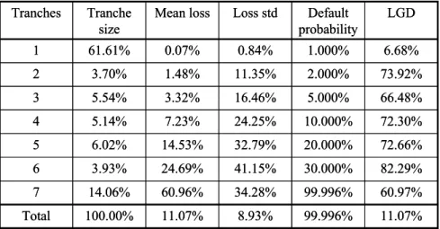
Table 1: Summary statistics for tranches

This table presents sum m ary statistics for the seven tranches, representing claim s of strict sub ordi-nation on the underlying p ortfolio. The statistics indicate the allo cation of losses of the underlying p ortfolio to the individual tranches. The cut-off values for a particular tranche is determ ined by the default probability allowed for that tranche as indicated in thefifth colum n. The m ost junior tranche (tranche numb er 7) corresp onds to thefirst loss piece. It b ears all losses not covered by the other, m ore senior, tranches. The colum ns present, from left to right, the tranche numb er, the tranche size, m ean loss, loss standard deviation, default probability, and loss given default. The last row displays the statistics for the underlying p ortfolio.

82.29% 30.000% 41.15% 24.69% 3.93% 6 99.996% 99.996% 20.000% 10.000% 5.000% 2.000% 1.000% Default probability 11.07% 8.93% 11.07% 100.00% Total 60.97% 34.28% 60.96% 14.06% 7 72.66% 32.79% 14.53% 6.02% 5 72.30% 24.25% 7.23% 5.14% 4 66.48% 16.46% 3.32% 5.54% 3 73.92% 11.35% 1.48% 3.70% 2 6.68% 0.84% 0.07% 61.61% 1 LGD Loss std Mean loss Tranche size Tranches 82.29% 30.000% 41.15% 24.69% 3.93% 6 99.996% 99.996% 20.000% 10.000% 5.000% 2.000% 1.000% Default probability 11.07% 8.93% 11.07% 100.00% Total 60.97% 34.28% 60.96% 14.06% 7 72.66% 32.79% 14.53% 6.02% 5 72.30% 24.25% 7.23% 5.14% 4 66.48% 16.46% 3.32% 5.54% 3 73.92% 11.35% 1.48% 3.70% 2 6.68% 0.84% 0.07% 61.61% 1 LGD Loss std Mean loss Tranche size Tranches

Applying the loss distribution of the total portfolio leads to the following tranche sizes starting from the most senior tranche: 0.6161, 0.0370, 0.0554, 0.0514, 0.0602, 0.0393, and 0.1406 for the equity piece. Further summary statistics for the tranches are provided in Table 1. Graphical representations of the loss

distributions for different tranches (senior tranche, mezzanine tranche, andfirst

loss piece) are given in Figure 2.

In Table 1, the senior tranche is by far the largest part of the entire trans-action, making up 61.61% of the transaction. The expected loss rate is only 7 basis points, while expected loss given a default event is 668 basis points. The mean loss rate is monotonously increasing in the degree of subordination. Its maximum value is 60.96% for the equity piece. The default probability of the equity piece is almost 100%, as there were only 2 out of 50’000 runs in the simulation that came out with a zero loss rate for the entire portfolio.

The numbers for the senior tranche are particularly striking, as they show a very low loss given default rate, despite its large size. Figure 2 explains why this is the case. Realized portfolio losses that surpass the capacities of the

Figure 2: Loss distribution of tranches

This diagram presents the loss distribution of three tranches (from left to right): thefirst loss piece (tranche 7), a m ezzanine tranche (tranche 6), and the senior tranche (tranche 1). The calculations are p erform ed with 50’000 simulation runs. The horizontal axis shows the loss rate; the vertical axis shows the observed frequency, truncated at 30% , 1% , and 0.2% , resp ectively. There are several values surpassing these thresholds: For thefirst loss piece, 100% loss occurs at a frequency of 30% . For the m ezzanine tranche, zero loss o ccurs at a frequency of 70% , and 100% loss o ccurs at a frequency of 20% . For the senior tranche, zero loss o ccurs at a frequency of 99% .

0% 5% 10% 15% 20% 25% 30% 0% 20% 40% 60% 80% 100% 0.0% 0.5% 1.0% 0% 20% 40% 60% 80% 100% 0.0% 0.1% 0.2% 0% 20% 40% 60% 80% 100%

more subordinate tranches cluster at the low end of possible loss rates, without any observation exceeding a 25% loss rate in the simulation runs. Clearly, the distribution of losses in this tranche is sensitive to the extreme-value properties

of the underlying risk factors3_.

As can be seen from Figure 2, the most subordinate mezzanine tranche, no. 6, displays a broad tendency of a downward sloping distribution func-tion throughout its domain. While the loss rate distribufunc-tions for all mezzanine tranches are downward sloping, their slope decreases with the degree of seniority of the tranche in question for standard portfolio loss distributions and standard

cut-offvalues for tranches.

The distribution of thefirst loss piece, depicted in Figure 2, is single peaked

in the interior of its domain, abstracting from the spike at its upper boundary. This follows from the fact that the lowest tranche comprises two thirds of the cumulative loss rate distribution, comprising the peak of the aggregate loss rate distribution.

From the simulation exercise we obtain a couple of insights. By tranching, the risks of the underlying portfolio are allocated in a non-proportional way to the tranches. The loan portfolio is transformed into several securities with

entirely different risk characteristics. The tranches or only a selection of them,

as is often intended, can subsequently be sold independently to investors. The senior tranche has the highest quality in all categories. The probability of default is lowest, with no loss in 99% of all cases in this example. In addition, mean loss, loss standard deviation, and loss given default are lowest among all tranches.

3_{This points at a natural extension of our analysis, which uses fat-tailed distributions to}

Furthermore, the senior tranche is by far the largest of all tranches, with a claim on 61.61% of the volume of the underlying portfolio. In contrast to the senior

tranche, thefirst loss piece suffers a loss rate of 100% with a large probability of

30%. Furthermore, while low losses occur at low frequency, higher losses occur with an increasing likelihood, peaking at a loss of 22%. Overall, the FLP has the highest expected loss of all tranches. Finally, the presented statistics illustrate that even reference portfolios of relatively bad quality (20% default probability over 1 year for all loans in this case) can be divided into one large tranche of

the highest quality, a couple of mezzanine tranches, and a relatively smallfirst

loss piece in which the major proportion of credit risk is concentrated.

3.2

Tranche interdependencies

In this section, we use the data generated in the simulation exercise in order to investigate the correlation between tranches. Since the underlying structural

model differentiates between macoeconomic and idiosyncratic risk, we will now

use the risk model presented in the pevious section in order to identify the exposure of single tranches to the macroeconomic risk factor. The analysis shows that non-proportional risk sharing allocates macro risk primarily to junior

tranches. In a first step, the correlation between tranches of a single issue is

analyzed, e.g, the correlation between thefirst loss piece that is retained on the

bank’s balance sheet and a mezzanine or a senior tranche of the issue. In a second

step, we look at tranches of different issues, e.g. the correlation between two

first loss pieces, or two senior tranches with distinct underlying asset portfolios.

Since we control the data generating process, we can trace the effect of changes

in the underlying asset correlations to the resulting tranche correlations. Table 2 displays the bilateral correlations of all CDO tranches (ranging from

senior tranche to thefirst loss piece). The results indicate that tranches of

simi-lar credit quality, or seniority, have higher correlation values than tranches with

different credit quality. The correlation between tranches of a given transaction

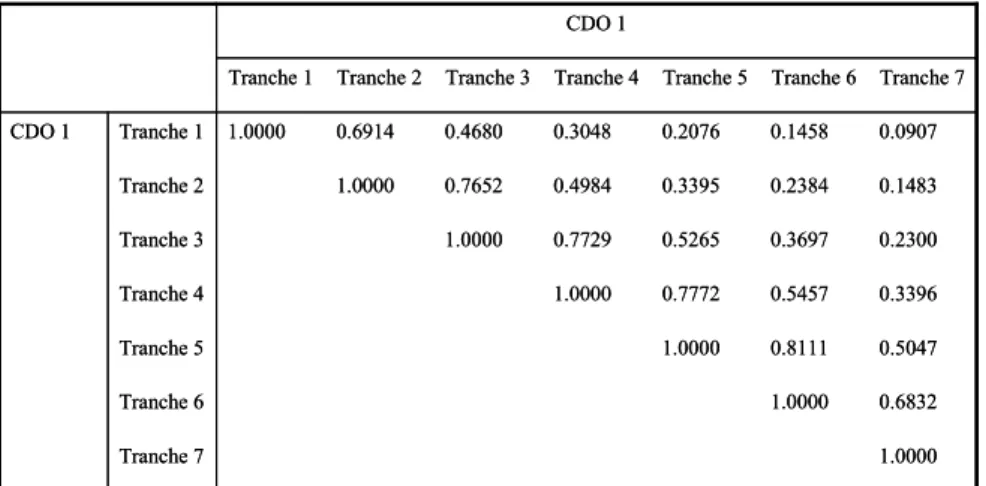
(CDO 1 in Table 2) decreases monotonically with the distance of quality of two tranches (or tranche numbers, for that purpose). The correlation of tranche #1, the senior tranche, with the most junior tranche #7, the equity piece, is 0.0907. This shows that senior tranches are almost orthogonal to junior tranches, in par-ticular to the equity piece. Note that even lower correlations can be attained by increasing the distance of tranches, e.g. by decreasing the maximum default probability allowed for the senior tranche.

In Table 3, the tranche-correlations of two CDOs with identical characteris-tics are displayed. The correlation values are the higher the more similar are the tranches with respect to seniority. The highest correlation values are obtained for tranches with the same credit quality. These values are close to one. Cor-respondingly, the lowest bilateral correlation values are obtained for the most senior and the most junior tranches (0.0906). Note that for large portfolios, the correlation pattern converges in the limit to that of same-issue tranches (see Table 2). Correspondingly, if the reference portfolios have less obligors, the

Table 2: Bilateral correlations of all tranches from one CDO issue

This table displays the bilateral correlations of all CDO tranches ranging from tranche numb er 1 (m ost senior tranche) to tranche numb er 7 (first loss piece). The reference p ortfolio consists of 10’000 loans, and all of them have a default probability of 20% , 1 year m aturity, 47.5% recovery rate, and 6% coup on. All loans are assum ed to have a default correlation of 0.3. All cash flows are discounted with a constant interest rate of 4% . The loss distribution is calculated with 50’000 simulations. 1.0000 Tranche 7 0.6832 1.0000 Tranche 6 0.5047 0.8111 1.0000 Tranche 5 0.3396 0.5457 0.7772 1.0000 Tranche 4 0.2300 0.3697 0.5265 0.7729 1.0000 Tranche 3 0.1483 0.2384 0.3395 0.4984 0.7652 1.0000 Tranche 2 0.0907 0.1458 0.2076 0.3048 0.4680 0.6914 1.0000 Tranche 1 CDO 1 Tranche 7 Tranche 6 Tranche 5 Tranche 4 Tranche 3 Tranche 2 Tranche 1 CDO 1 1.0000 Tranche 7 0.6832 1.0000 Tranche 6 0.5047 0.8111 1.0000 Tranche 5 0.3396 0.5457 0.7772 1.0000 Tranche 4 0.2300 0.3697 0.5265 0.7729 1.0000 Tranche 3 0.1483 0.2384 0.3395 0.4984 0.7652 1.0000 Tranche 2 0.0907 0.1458 0.2076 0.3048 0.4680 0.6914 1.0000 Tranche 1 CDO 1 Tranche 7 Tranche 6 Tranche 5 Tranche 4 Tranche 3 Tranche 2 Tranche 1 CDO 1

Table 3: Bilateral correlations of tranches from two different CDO issues

This table displays the bilateral correlations of all tranches from two different CDO issues ranging from tranche numb er 1 (m ost senior tranche) to tranche numb er 7 (first loss piece). Both CDO s have sim ilar characteristics: The reference p ortfolios consist of 100 loans, and all of them have an initial rating of BB, 1 year m aturity, 47.5% recovery rate, and 6% coup on. All loans are assum ed to have a default correlation of 0.3. All cashflows are discounted with a constant interest rate of 4% . The loss distribution is calculated with 50’000 simulations.

0.9991 Tranche 7 0.6824 0.9978 Tranche 6 0.5041 0.8113 0.9982 Tranche 5 0.3392 0.5459 0.7764 0.9976 Tranche 4 0.2298 0.3698 0.5260 0.7718 0.9972 Tranche 3 0.1482 0.2385 0.3392 0.4977 0.7638 0.9964 Tranche 2 0.0906 0.1458 0.2074 0.3044 0.4672 0.6896 0.9977 Tranche 1 CDO 1 Tranche 7 Tranche 6 Tranche 5 Tranche 4 Tranche 3 Tranche 2 Tranche 1 CDO 2 0.9991 Tranche 7 0.6824 0.9978 Tranche 6 0.5041 0.8113 0.9982 Tranche 5 0.3392 0.5459 0.7764 0.9976 Tranche 4 0.2298 0.3698 0.5260 0.7718 0.9972 Tranche 3 0.1482 0.2385 0.3392 0.4977 0.7638 0.9964 Tranche 2 0.0906 0.1458 0.2074 0.3044 0.4672 0.6896 0.9977 Tranche 1 CDO 1 Tranche 7 Tranche 6 Tranche 5 Tranche 4 Tranche 3 Tranche 2 Tranche 1 CDO 2

According to these simulations, the results confirm that portfolio risk is transferred to tranches in a non-linear way. In particular, the risk associated with senior tranches is only to a minor extent correlated with the risk that

remains on the bank’s balance sheet, given the retention of thefirst loss piece.

This raises the question to what extent this result depends on the diversification

among the assets in the underlying loan portfolio. We turn to this question next.

3.3

Estimating the systematic risk of tranches

The objective of the analysis is to trace the effect of macroeconomic risk to

the risk exposure of individual tranches, structured according to the principle of subordination. This section has an important result: under quite general as-sumptions about tranching, the most subordinate tranche has the largest macro-factor dependency. Tranching therefore tends to increase an issuers systematic equity risk, provided the most junior tranche is retained, a wide-spread industry practice. To capture the impact of systematic risk on tranches, we consider a bond that only depends on the macroeconomic factor and does not exhibit any idiosyncratic risk. This bond, which we call a macro bond, is assumed to have otherwise identical characteristics to the bonds in the portfolio, i.e. 1 year to maturity, 6% coupon, 20% default rate, and 47.5% recovery rate. The macro bond allows us to estimate directly the relationship between the macro risk fac-tor and the realizations of particular tranches of an underlying loan portfolio. In our setting of normally distributed realizations, the default rate of 20% cor-responds to a default boundary of -0.8416 according to the distribution function

of (macro bond) value realizationsVn,tin Eq. (1), whereρMn is set equal to one.

Table4summarizes the results, comparing joint default events of the tranches

and the macro bond. The second column reports the unconditional default rates

of the tranches, as specified for the simulation in this paper. The third column

reports the default rate of the tranche conditional on the default of the macro bond. This conditional tranche default rate is monotonic in the tranche quality, leading to the highest value of 100% for the most junior tranche, and to 4.95% for the most senior tranche. Note that these conditional default probailities are almost four times higher than the unconditional probabilities for tranches 1 to 5.

The fourth column specifies the conditional macro bond default rate, i.e. the

probability of a macro bond default, given the default of a particular tranche. This conditional default rate is 100% for all senior tranches, and gradually

decreases for junior tranches. For the first loss piece, the conditional default

rate is lowest, with a value of 20.15% in our simulation.

The results in Table 4 show that the impact of macro risk on the default

rates of tranches varies systematically with the rating quality of the tranche. According to the last column, the more senior a tranche is, the more likely is its default accompanied by a negative realization of the macro risk factor.

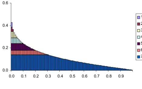
Figure3relates tranche losses to realizations of the macro factor. Thefirst

loss piece suffers losses even for very good realizations of the macro factor. The

Table 4: The effect of systematic risk on tranches

This table presents the effect of system atic risk on tranches. All loans are assum ed to have a default correlation of 0.3, a default probability of 20% , 1 year m aturity, 47.5% recovery rate, and 6% coup on. All cashflows are discounted with a constant interest rate of 4% . The calculations are p erform ed with 50’000 simulation runs. Thefirst colum n shows the tranches considered, ranging from 1 (m ost senior tranche) to 7 (first loss piece). The second colum n rep orts the unconditional default rates of the tranches. The third colum n rep orts the default rate of each tranche conditional on the default of a b ond only sub ject to m acro econom ic risk. The fourth colum n sp ecifies the probability of a m acro b ond default, given the default of a particular tranche.

100.00% 100.00% 30.00% 20.00% 10.00% 5.00% 2.00% 1.00% Pd_(tranche) 100.00% 100.00% 100.00% 98.42% 49.61% 24.80% 9.92% 4.95% Pd_{(tranche | macro)} 20.15% Total portfolio 20.15% 7 67.21% 6 99.22% 5 100.00% 4 100.00% 3 100.00% 2 100.00% 1 Pd_{(macro | tranche)} Tranche 100.00% 100.00% 30.00% 20.00% 10.00% 5.00% 2.00% 1.00% Pd_(tranche) 100.00% 100.00% 100.00% 98.42% 49.61% 24.80% 9.92% 4.95% Pd_{(tranche | macro)} 20.15% Total portfolio 20.15% 7 67.21% 6 99.22% 5 100.00% 4 100.00% 3 100.00% 2 100.00% 1 Pd_{(macro | tranche)} Tranche

around the 30 percent quantile. For lower realizations, the losses of the first

loss piece are truncated at its share of the reference portfolio, corresponding to

a loss of 100 percent. In constrast to thefirst loss piece, the senior tranche only

suffers losses in the case of extremely bad realizations of the macro factor. Note

that the senior tranche even in the worst case only suffers minor losses although

it has by far the largest size of all tranches. This is due to the recovery that truncates losses of the senior tranche.

We now turn to the estimation of a central measure of tranche interdepen-dency on a market, which is beta, the systematic risk of individual tranches. This measure of risk is used in portfolio theory to capture the degree of pro-cyclicality of two random variables. A beta value larger (smaller) than one characterizes a return series that exhibits more (less) cyclical variation then the

benchmark index. In calculating tranche betas we take the macro factorYt

M as

the benchmark index. Table5shows the sensitivity of the individual tranches

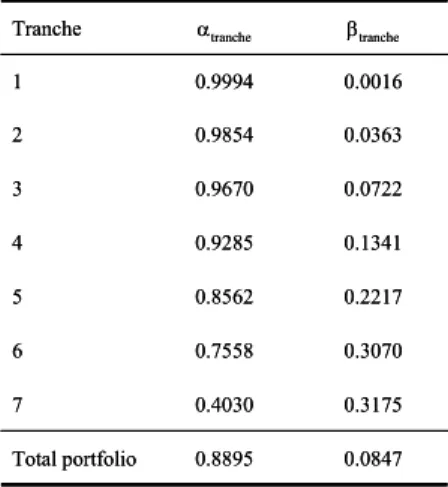
to the macro risk factor. In particular, the realized tranche returns obtained in the simulation runs are regressed on the macro risk factor. The estimated betas

increase monotonically with the level of subordination, indicating that thefirst

loss piece has a high sensitivity to the macro risk factor while the most senior

tranche almost has none. Thus, with tranches being exposed to different degrees

of systematic risk, also the exposure of the issuing institution to systematic risk changes in the practically relevant case that not all tranches are sold.

Figure 3: Tranche sensitivity to macro factor

Thisfigure shows the sensitivity of individual tranches to realizations of the m acro factor. The tranche numb ers range from 1 (senior tranche) to 7 (equity piece). The vertical axis shows the loss rate with resp ect to the reference p ortfolio. The vertical axis shows the quantiles of m acro factor realizations. High quantiles indicate go od states of the economy.

0.0 0.2 0.4 0.6 0.0 0.1 0.2 0.3 0.4 0.5 0.6 0.7 0.8 0.9 1 2 3 4 5 6 7

Table 5: Tranche beta

This table presents the results from a regression relating tranche returns to the corresp onding realizations of the m acro econom ic factor. All loans are assum ed to have a default correlation of 0.3, a default probability of 20% , 1 year m aturity, 47.5% recovery rate, and 6% coup on. All cashflows are discounted with a constant interest rate of 4% . The calculations are p erform ed with 50’000 simulation runs. The first colum n shows the tranches considered, ranging from 1 (m ost senior tranche) to 7 (first loss piece). The second colum n rep orts the alpha values and the third colum n rep orts b eta values of the regressionr=α+β∗YM+ .

0.8895 0.4030 0.7558 0.8562 0.9285 0.9670 0.9854 0.9994 αtranche 0.0847 0.3175 0.3070 0.2217 0.1341 0.0722 0.0363 0.0016 βtranche Total portfolio 7 6 5 4 3 2 1 Tranche 0.8895 0.4030 0.7558 0.8562 0.9285 0.9670 0.9854 0.9994 αtranche 0.0847 0.3175 0.3070 0.2217 0.1341 0.0722 0.0363 0.0016 βtranche Total portfolio 7 6 5 4 3 2 1 Tranche

4

Implications for Bank Risk

In this section, we investigate the risk position of a bank that issues a CDO,

assuming that it retains thefirst loss piece, the most junior tranche. We make

this assumption since it is believed to be common practice among international banks. We have no direct evidence supporting this assumption and therefore refer to survey results (See ECB 2004 and Bundesbank 2004). This section shows that under fairly general assumptions concerning bank reinvestment behavior, risk transfer will simultaneously decrease its exposure vis-à-vis extreme risks and increase its overall macro-factor dependence. We therefore predict issuing banks to increase their equity beta.

4.1

Securitization and reinvestment

We now investigate the risk position of a bank that issues CDOs. Typically, a bank is exposed to various types of risk, in particular market risk, credit

risk, and operational risk. Market risk is often defined as outcomes from

po-sition taking (stock, interest-sensitive securities, foreign exchange) as well as customer-related activities (fees and provision). Credit risk incurs from lending

which generates fees and interest income. Finally, operational risk as defined

by the Basle Committee are losses due to external events and failure of internal processes, people, or systems. The distributions of all mentioned sources of risk have distinct characteristics. Market risk is typically assumed to have a sym-metric distribution with a high variance, operational risk is typically assumed to have a very thin distribution with large tails, and credit risk is assumed to have a skewed distribution with limited gains, but unlimited loss potential. On average, the banks’ exposure to credit risk is about 6.5 times higher than to market risk, as obtained by [19], and thus the distribution of credit risk has a dominating impact on the overall risk distribution of a bank. What is the resulting risk position of a bank that actively securitizes its loan portfolio?

The impact of securitization on overall bank risk crucially depends on how

the proceeds are reinvested. The resulting effect is not obvious as there is a whole

range of possiblilties. In the extreme case on the one side, the balance sheet of the bank risk is levered, either by distributing the proceeds to shareholders or by entering new investments with similar risk characteristics as the retained junior tranche. In the other extreme, overall bank risk also can decrease with a securitization transaction. This is the case when the proceeds are invested in new projects with lower risk. Thus, depending on the new risk position following securitization and re-investment, a bank will have to hold more or less equity according the capital accords of the Basle committee. Seen from a dynamic

perspective, the bank will either be exposed more or less to thefluctuations of

the overall economy. Thus, while the Basle 2 accords have pro-cyclical effects,

securitization (and re-investment) allows to influence a bank’s risk sensitivity to

the overall economy and thereby the capital requirements. Thus, securitization allows banks to pursue its lending business independently of the state of the

Figure 4: Loss distribution of a loan portfolio after repeated securitizations and reinvestments

Thisfigure shows the loss distribution of a loan p ortfolio after rep eated securitizations and rein-vestm ents. The original p ortfolio is securitized by retaining afirst loss piece of 14.06 p ercent. The proceeds obtained from the securitized p ortion (85.94 p ercent of the initial p ortfolio) am ount to 94.26 p ercent of the total p ortfolio value as obtained with a one-factor asset pricing m o del. This am ount is reinvested in a new p ortfolio consisting of identical loans. Loss distributions are shown for several iterations ranging from zero (the original p ortfolio is kept) to infinity (the lim it case). The horizontal axis shows the loss incurred with resp ect to the initial p ortfolio value, determ ined with a one-factor asset pricing m o del. Negative values indicate excess returns. The vertical axis shows the frequency of relative losses.

0% 5% 10% 15% 20% 25% 30% 35% -200% -100% 0% 100% 0 1 2 10 lim

To determine the resulting risk position of a bank that actively securitizes its loan portfolio, we investigate the special case of a bank that repeatedly securitizes its loan portfolio and reinvests the proceeds. It turns out that a bank that repeatedly securitizes its loan portfolio and reinvests the proceeds

will have an entirely different risk position after these transactions. With each

iteration, the bank increases its leverage. Figure 4 shows the credit risk exposure

of a bank that repeatedly securitizes its loan portfolio, retains thefirst loss piece

and reinvests the proceeds in loans of the same quality characteristics in terms of loss distribution. We start out from a simulated loss distribution obtained for a benchmark portfolio with 10’000 individual loans and 1 year to maturity. The default probability of the loans in the portfolio is 20%, and the recovery rate in case of default is 47.5%. Applying the Monte Carlo Simulation technique to this portfolio leads to the distribution of the original portfolio. The obtained average loss rate is 11.07% with a standard deviation of 8.93%.

After every round of securitizing and reinvesting, the resulting relative loss distribution of the bank changes with the number of iterations and takes a

dis-tinct shape, differing from that traditionally assumed for credit risk exposures.

This has important implications for firm-wide risk management of the bank.

Repeated securitization and reinvestment uniformly increases the return vari-ance of the securitizing bank and the value-at-risk. The special case of identical loss rate distribution for the initial loan portfolio and all new (reinvested) loan portfolios has a simple limit result: the loss distribution of the portfolio with

repeated reinvestment converges to that of the originalfirst loss piece. However,

even a small number of iterations transforms the bank’s loss rate distribution substantially, reducing its skewness and increasing its mean value. Already after one round, mean loss rate and standard deviation increase substantially and take the values 18.09% and 12.07%, respectively. The limit distribution has a mean loss rate of 60.96% and a standard deviation of 34.28%, while the probability of a complete asset loss is 30% (compared to 0.00% in the original portfolio). This latter number is also the probability that the bank goes bankrupt provided

that it is completely equityfinanced and has no additional income from sources

other than lending. The results are important for bank risk management and regulation likewise.

4.2

Estimating the e

ff

ect of granularity

In this section, we investigate the effect of increasing granularity on the standard

deviation of the asset portfolio. We will trace the effect of diversification on the

average correlation by varying the number of assets (loans) in the underlying

pool. We carry out this basic test, because we are interested in the effect of

securitization on diversification. One hypothesis advanced in the literature is

that a bank that engages in the transfer of risk through tranching increases

the diversification in its asset base. The reason is that the proceeds from a

securitization can be reinvested in new loans, thereby increasing the granularity of the loan book.

Table 6: The effect of portfolio diversification

This table presents, for three correlation scenarios, the standard deviation of losses for different numb ers of loans. The numb ers in parentheses indicate the reduction factor of the standard de-viation obtained when increasing the numb er of loans in the p ortfolio by the factor 10. In the three correlation scenarios, all loans are assum ed to have a default correlation of 0.0, 0.15, and 0.3, resp ectively. All loans have a default probability of 20% , 1 year to m aturity, 47.5% recovery rate, and 6% coup on. All cashflows are discounted with a constant interest rate of 4% . The calculations for the different p ortfolios are p erform ed with 50’000 simulation runs each.

6.16% (1.007) 6.21% (1.051) 6.52% (1.399) 9.12% (2.432) 22.19% Corr=0.15 10000 1000 100 10 1 Number of loans 0.22% (3.163) 0.70% (3.167) 2.21% (3.178) 7.04% (3.146) 22.13% Corr=0.0 Standard deviation 8.95% (1.004) 8.98% (1.023) 9.19% (1.198) 11.01% (2.017) 22.20% Corr=0.30 6.16% (1.007) 6.21% (1.051) 6.52% (1.399) 9.12% (2.432) 22.19% Corr=0.15 10000 1000 100 10 1 Number of loans 0.22% (3.163) 0.70% (3.167) 2.21% (3.178) 7.04% (3.146) 22.13% Corr=0.0 Standard deviation 8.95% (1.004) 8.98% (1.023) 9.19% (1.198) 11.01% (2.017) 22.20% Corr=0.30

have a default probability of 20%, 1 year to maturity, 47.5% recovery rate, and 6% coupon. Table 6 presents the standard deviation of losses after accounting for the number of loans. All loans are assumed to have a default correlation

of 0.0 and 0.3, respectively. The calculations for the different portfolios are

performed with 50’000 simulation runs each.

The results suggest that even a small number of loans in a portfolio is enough to diversify away the major part of idiosyncratic default risk. Consider the

first column. The asset base is assumed to consist of uncorrelated risks, and

the idiosyncratic risk (standard deviation) is 22.13%. If the number of loans

increases, the standard deviation of the portfolio loss rates is rapidly decreasing,

approaching zero. For example, with an asset base of 1000 loans, the resulting

portfolio standard deviation is reduced by 1₋ 0.7

22.13 = 96.84 percent, relative

to the original level, the standard deviation of the loss rate distribution of a single loan. As can be seen from columns 2 and 3, the decrease in standard deviation is a function of the bi-variate correlation between assets. For instance, if the correlation is 0.3, an asset base of 1000 loans reduces portfolio standard deviation to 8.98% of its original level. This number, however, is numerically close to portfolio standard deviation that can be reached when the asset base is decreased by a factor of 10. In this case, the resulting standard deviation is 9.19%, i.e. increases the standard deviation by a factor of 1.023 (+2.3%).

on portfolio standard deviation, provided the number of loans in the initial

portfolio exceeds 100. This exponential phasing out of the granularity effect

happens earlier (i.e. with a small number of loans in the initial portfolio) if the bi-variate loan correlation is high. For lower correlations, the phasing out

happens at higher degrees of granularity, but the overall effect is already close

to complete with merely 100 assets. The exception is a bi-variate correlation of 0.0, where the reduction of standard deviation for each increase of the number of loans by the factor 10, can be approximated by a constant factor, 3.1 in our simulations.

Overall, the results demonstrate that the diversification benefits are rapidly

decreasing with the number of securities in the portfolio. Typically, banks hold very large loan portfolios and the securitization of a bank’s loan book will only marginally increase asset granularity. Thus, contrary to what is often believed, securitizing a bank loan portfolio with subsequent reinvestment in new loans

will only have minor additional diversification benefits for banks.

4.3

Implications for bank beta

We now examine the effect of securitization on the exposure of banks to

system-atic risk. In particular, how does bank equity beta change in connection with a securitization transaction? For simplicity, we assume that a bank is only pursu-ing a lendpursu-ing business and that it has no other assets than its loan portfolio. On the other hand, the liabilities comprise equity and debt. We now examine how a bank’s beta changes with securitization, assuming that the bank securitizes its entire loan portfolio.

In line with the results obtained in Table 5, we assume that there is a

monotonous relation between the beta of a tranche and its seniority, and that the following inequality holds:

β_{F LP} > βorig_{P F} =βorig_assets,

whereβ_{F LP} is the beta of thefirst loss piece andβorig_{P F} is the beta of the original

reference portfolio.4

Generally, a bank’s asset- and equity-beta can be related by the following equation:

β_assets=β_debt·d+β_equity·e, (4)

whereβ_assets,β_debt, andβ_equityare the betas of the assets, debt, and equity,

respectively. The debt ratio is denoted byd, and the equity ratio is denoted by

e.

The relation between original and new bank equity beta can be expressed in a general way by using Eq. 4:

4_{Our simulation results show that the monotonous relation between the beta of a tranche}

and its seniority applies in all practically relevant cases. However, at this point, a formal proof of this assumption is left to the reader.

∆β_equity = βnew_equity−βorig_equity = β new assets enew − βorigassets eorig −

βnew_debt·dnew enew +

βorig_debt·dorig

eorig , (5)

where eorig _(dorig_{) is the original and e}new _(dnew_{) is the new equity (debt)}

ratio after securitization.

The new asset betaβnew_assetsdepends on how the securitization proceeds are

reinvested, i.e. which sensitivities the new securities have to the macroeconomic

risk factor. Lets denote the securitization proceeds in percent of the original

portfolio. Correspondingly, the percentage of the retained first loss piece is

equal to1₋s. Reinvestment also implies the possibility to pay out part of the

securitization proceeds to equity- or debtholders. Let the ratio of total payout

to total assets be represented byh. Thus, the new proportion of funds to be

reinvested is s∗ _≡ s−h

1−h, while the proportion of thefirst loss piece in the new

portfolio is1₋s∗ _≡ 1−s

1−h. Accounting for possible payout to equity- or

debt-holders, the new ratios∗ _{of reinvested funds. The new asset beta is then given}

by:

βnew_assets= (1₋s∗)_·β_{F LP} +s∗_·βreinvest. (6) By combining Eq. 5 and 6, we obtain a general formula for the relation

between original and new bank equity beta after securitization5_:

∆β_equity = (1−s ∗_)·β F LP +s∗·βreinvest enew − βorigassets eorig −

βnewdebt·dnew

enew +

βorig_debt·dorig

eorig ,

(7) Thus, magnitude and direction of equity beta change depend on bank lever-age before and after securitization as well as the beta of the reinvestment al-ternative chosen. Figure 5 shows in two panels the change in bank equity beta after a securitization transaction. The left diagram shows how equity beta

changes in response to different leverage, given a constant beta of reinvested

assetsβreinvest =βorig_assets. The plot shows that, for constant leverage, for

in-creasing leverage, and even for to some extent dein-creasing leverage, βnew_equity is

larger than βorig_equity. The right diagram shows how equity beta changes in

re-sponse to different beta of reinvested assets, given a constant equity ratio of 0.1

which is typical in the banking sector. The plot shows that equity beta rises in most cases and only decreases if the beta of reinvested assets is substantially below the beta of the original portfolio. Thus, we conclude that equity beta may rise or fall in response to a securitization transaction, but in most practically relevant cases, it will rise.

5_{Note that payouts may have any effect on firm leverage, ranging from an increase to a}

decrease, depending on how the payouts are distributed between equity- and debt-holders. Equally,firm leverage may also change without any payouts due to balance sheet restructur-ings.

Figure 5: Bank equity beta change after securitization

Thisfigure shows change of bank equity b eta after securitization for various values offirm leverage (panel a) and b eta of reinvested assets (panel b). The b eta of debt is set to zero. Thefirst loss piece has a share of 14.06 p ercent of the total p ortfolio. The b eta of the original p ortfolio as well as the reinvested securities is 0.0846, the b eta of thefirst loss piece is 0.3200, the original and the new equity ratios are 0.1, corresp onding to typical values for banks. In panel a, the new equity ratio is varied (vertical axis), in panel b, the b eta of the reinvested securities is varied (x-axis). In panel a, there is a p ositive (negative) change in equity b eta for equity ratios sm aller (larger) than 0.139. In panel b, there is a p ositive (negative) change in equity b eta for a weighted average b eta of reinvested securities larger (sm aller) than 0.046. Leaving b othfirm leverage and p ortfolio b eta of reinvested securities constant, the resultung equity b eta change of the bank is 0.3310.

-1 -0.5 0 0.5 1 0.0 0.1 0.2 0.3 0.4 0.5 0.6 0.7 0.8 0.9 1.0 -0.6 -0.4 -0.2 0 0.2 0.4 0.6 0.8 1 0.00 0.05 0.10 0.15 0.20

It is worth noting that there is a substantial difference between synthetic and

true sale transactions with respect to the change in equity beta. The argument as outlined above, i.e. that beta may rise or fall in response to a securitization transaction, holds for true sale transactions. In the case of synthetic transac-tions, however, the argument changes: Since all claims are settled at maturity,

there are no immediate cashflows from the transaction that can be reinvested

in new securities or distributed to equity- or debt-holders. Consequently, in the case of synthetic transactions, there will always be an increase in equity beta.

The analysis presented in this paper builds on a one-factor macroeconomic risk model. In extended versions with several independent risk factors, the results remain essentially unchanged. There are only more sensitivities and beta changes that have to be considered, each likewise represented by Eq. 7.

5

Systemic Risk

In the last section we have established that under certain conditions relating to

the retention offirst loss pieces, the securitization of a loan portfolios by a bank

will lead to an increase in its exposure to market risk. We found the increase of the issuing institution’s systematic risk to be positively related to the size of the retained equity piece, and to the reinvestment beta of the issue proceeds. Beta always increases for synthetic issues, since there are no issue proceeds.

All these claims pertain to the individual bank. What do they imply for the banking sector as a whole? On the basis of the simple risk transfer model introduced in this paper, we now estimate the correlation of defaults. This

corresponds to a widely used definition of systemic risk, the likelihood of a

concurrent failure of several banks, see Kaufman (2000) or Lehar (2005).6 _For

any given joint loss rate distribution, one can determine the cumulative density

of a certain number n or more banks defaulting simultaneously. This will be

our approach to capture system-wide default risks, and we will investigate the relationship between systematic risk exposure on the level of the individual bank and its contribution to the risk of multiple bank failures.

5.1

How securitization a

ff

ects joint default probabilities

The previous section has concluded that the securitization of a bank’s loan portfolio combined with the retention of a junior claim on the asset pool, tends to raise the bank’s equity beta. Therefore one may ask: What is the marginal

effect of such a beta rise on the likelihood of multiple bank failure? To answer

this question we run a Monte Carlo simulation with many banks, all modeled as in section 4. We let one bank securitize its loan portfolio, tranching the portfolio according to the rules outlined in section 3, selling all tranches except the most subordinate one, and reinvesting the proceeds in assets of a similar quality as

the securitized loan portfolio7_.

Table 7 shows, for a market consisting of 5 banks, the probability that a certain number of banks default. In the base case of no securitization, i.e. all banks holding on to their original loan portfolios, the probability of at least one bank defaulting amounts to 42.13% while the probability that all banks default amounts to 39.88%. Thus, in the majority of all cases, either all banks or no

bank will default.8

Table 7 compares the performance of banks and shows the probabilities of at least 1, 2, ..., 5 banks defaulting simultaneously. The numbers reported

are cumulative probabilities. Thefirst column shows the base case, when no

bank securitizes its loan portfolio. In this case, the probability of just one bank

6_{Kaufman (2000) surveys the many different definitions of systemic risk used in the}

liter-ature. These definitions have received considerable attention, probably because the contain-ment of systemic risk is one of the core justifications for banking supervision, and for central bank interventions infinancial markets.

7_{The assumption that new loans have similar characteristics as the old loans is for ease of}

exposition only. In section 4, it was shown that the change in macro factor exposure has the predicted same sign as long as the reinvestment beta is not too much smaller than the beta of the original loan portfolio. So, for instance, the re-investment of ABS proceeds in riskless government bonds could actually lower the issuing banks equity beta. If this is the case, the effect on systemic risk is the other way around.

8_{Note that the number of bank defaults is dominated by the realization of the macro factor}

in this example. The dominance of macro factor realizations is due to (1) the large size of the loan portfolios with 10000 loans each and (2) the rather high correlation assumption of 0.3 between all loans. However, our calculations for more realistic average correlations show that the numbers do not change much. Still, realizations of the macro factor dominate the results, i.e. in the majority of all cases, either all banks or no bank default.

defaulting is 42,13%, in line with the high individual default probability assumed in these simulations (see section 4 for details). Changing the individual default probabilities will downshift the numbers in column 1 as well. The second column

reports the effect of one securitizing bank on the joint default probabilities of

1,...,5 banks. There is a uniform increase in system-wide joint default probability

for the different levels of joint default in Table 7. The third column assumes

that all five banks engage in one round of asset securitization. The numbers

in the table indicate that securitization increases the risk of joint bank defaults at each level, represented by the minimum number of banks jointly defaulting. While the probability that at least one bank defaults is 42.13% if all banks hold on to the original loan portfolio, the default probability increases to 56.05% if all

banks sell offtheir loan portfolios, retaining thefirst-loss piece, and reinvest the

proceeds in new loans. Similar increases can be observed for all other levels of systemic risk, i.e. that at least 2, 3, 4, or 5 banks default. Correspondingly, the

probability of a joint default of allfive banks rises by 14.15 percentage points

in comparison to the base case of no securitization and reaches 54.03%. The results reported in Table 7 support the claim that asset securitization may increase the systematic risk exposure of these banks. Furthermore, the risk

transfer by even a singlefinancial institution will contribute to an increase of

the systemic risk of the banking sector. Note that the source of systemic risk in our model is not contagion, or any other inter-bank liability, but the impact of

a common macroeconomic factor in the return generating process9_{. The reason}

why securitization levers macroeconomic risk has been shown in this and the

previous section: it is the influence that securitization (or structured funding in

general) exerts on the systematic risk of the bank’s asset composition. In our

simulations, this influence is due to a) the retention of the most subordinate

tranche, and b) to the characteristics of the reinvestment decision concerning the generated new funds.

Overall, these results show how the mechanics of tranching and securitization relate to systemic risk, providing a framework for more precise regulation.

5.2

Inferring systemic risk from market betas

In the previous section, we have shown that by the use of collateralized debt obligations, based on the mechanics of tranching and securitization, banks may increase their systematic risk, and thereby may raise the stability risk of the

financial system at large. We have captured the bank’s macro factor exposure

by beta, the bank return’s standardized covariance with the volatility of the market index. We now turn our approach on its head and analyze whether or not a change of a bank’s equity beta is an indicator of an increased systemic

banking risk. This question is important, since an affirmative answer would give

us an easy-to-use instrument at hand that allows the monitoring of joint bank default rates, or synonymously, systemic risk. On the other hand, the question

9_{In the recent literature on systemic bank risk, there is an emphasis on inter-bankfinancial}

relationships as the main source of systemic risk, see De Bandt and Hartmann (2002) for a survey.

Table 7: Multiple bank defaults

This table shows the probability of multiple bank defaults. The exam ined m arket consists of 5 banks holding loan p ortfolios from different obligors, but with otherwise identical characteristics. The given numb ers are probabilities that at least a certain numb er of banks in the m arket default. The default probabilities are given for three scenarios: (1) no bank securitizes, i.e. all banks hold on to their original loan p ortfolios, (2) one bank securitizes its loan p ortfolio, retaining thefirst-loss piece and reinvesting the proceeds, and (3) all banks securitize their loan p ortfolios.

40.00% 40.69% 41.27% 42.01% 55.04% One bank securitizes 54.03% 39.88% 5 54.60% 40.49% 4 55.05% 40.98% 3 55.46% 41.47% 2 56.05% 42.13% 1 All banks securitize No bank securitizes Minimum number of bank defaults 40.00% 40.69% 41.27% 42.01% 55.04% One bank securitizes 54.03% 39.88% 5 54.60% 40.49% 4 55.05% 40.98% 3 55.46% 41.47% 2 56.05% 42.13% 1 All banks securitize No bank securitizes Minimum number of bank defaults

is not trivial, because it is conceivable that a) securitizations lead to increased

systematic and systemic risk, as shown in sections 4 and 5, and b) both effects

are actually a consequence of the bank retaining the highly riskyfirst loss piece

of the securitization. Thus, the increase in systemic risk reported earlier, may

be due to the specific risk allocation achieved in structuredfinance, but it may

not be caused by an increase in beta itself. To put it differently, in this section

we will analyze whether an increase in beta will always increase the joint default probability of banks, independent of the reason for the shift in beta.

Table 7 reports the results of a Monte Carlo simulation withfive banks, all

of which have the same characteristics (equity ratio of 10%, default probability of 10%, and equal betas). However, in contrast to earlier simulations, we do not assume anything about securitization and reinvestment. Instead, we model the bank as a return generating entity with a given macro risk exposure, summarized

by its beta value. We look at three distinct scenarios. In thefirst scenario, all

banks have a zero macro factor exposure, i.e. each individual beta is equal to zero. Results are in col.1 of Table 7.

We find a rapid decay in the probability of joint bank defaults for higher

numbers of banks involved. Thus, the probability of one bank or more failing is 40.55%, while it is 7.96% for two or more and 0.05% for 4 or 5 banks failing jointly. If we increase beta uniformly to the level of 1, the probabilities for more than one bank failure is rising for all levels of systemic crisis, relative to the base case in col.1. Only the probability of just one bank failure is reduced, indicating that probability mass is shifted from independent default occurrence

Table 8: Systemic risk and beta

This table shows the probability of multiple bank defaults. The exam ined m arket consists of 5 banks holding loan p ortfolios from different obligors, but with otherwise identical characteristics. The given numb ers are probabilities that at least a certain numb er of banks in the m arket default. The default probabilities are given for three scenarios with different bank equity b etas. The tuples in thefirst row indicate the equity-b eta values of each of the 5 banks in the m arket.

0.00% 0.05% 0.84% 7.96% 40.55% (0,0,0,0,0) 0.01% 0.10% 1.20% 8.78% 39.76% (1,1,1,1,1) 0.01% 5 0.17% 4 1.58% 3 9.49% 2 38.55% 1 (2,2,2,2,2) Minimum number of bank defaults 0.00% 0.05% 0.84% 7.96% 40.55% (0,0,0,0,0) 0.01% 0.10% 1.20% 8.78% 39.76% (1,1,1,1,1) 0.01% 5 0.17% 4 1.58% 3 9.49% 2 38.55% 1 (2,2,2,2,2) Minimum number of bank defaults

even higher systemic risk, i.e., the likelihood of multiple bank failures rises at all levels. Here again, the probability of a single bank failure is reduced, due to increased macro factor dependence. Thus, a unanimous increase in equity beta for all banks leads to a higher probability of multiple bank defaults.

Summing up, we we showed how bank equity betas relate to the probability

of multiple bank defaults. In particular, wefind support for the hypothesis that

individual bank equity betas are an important statistic for multiple bank failure risk.

6

Conclusion

This paper traces the effect of a financial innovation on the risk profile of an

individual bank, and more generally on the stability of the banking sector.

Thefinancial innovation we are looking at is the securitization of the loan book.

Throughout the paper, we employ numerical methods, which allows us to closely examine the nature of risk transfer.

The key finding in this paper is a positive relationship between

subordi-nation and macro factor dependence. We find senior tranches to have a low

correlation with the macrofactor, while junior tranches have substantial posi-tive correlation, far higher than the underlying asset portfolio itself. This result implies that under plausible conditions concerning the properties of the

under-lying credit assets and the retention of thefirst loss piece, the systematic risk of

the issuing bank, as measured by its equity beta, will rise. To derive this result we have projected the portfolio default rate of individual tranches on a macro risk factor, which in turn served to generate the returns of the individual loans,