Valuation and Optimization of Credit Risk using a Portfolio Model

(1)

Valuation and optimization of credit risk using a

portfolio model

Per Sidén

2012-09-30

(2)

Abstract

In this paper I study a model for credit risk in a portfolio of sovereign bonds, based on (van der Hoorn, 2009). The model is based on historical credit rating changes and the joint distribution of the losses for dier-ent bonds is modeled with an assumption of an underlying multivariate Gaussian variable. Dierent risk measures for the portfolio are calculated using Monte Carlo simulations and the performance is improved by the use of importance sampling. I investigate dierent methods on how to improve the model and the estimation of the parameters of the model. I also develop methods to valuate the certainty of the risk measures based on a statistical view on the input data, which give clear indications that the small size of input data gives low accuracy for the risk measures. An attempt to write an algorithm to nd the optimal portfolio with respect to the risk measures is also performed and the results are discussed.

(3)

Acknowledgements

I would like to thank my supervisor at Sveriges Riksbank, Tomas Edlund, for all his help and guidance throughout this thesis. I would also like to thank Jimmy Olsson at Lunds University and Kristofer Björnström at Sveriges Riksbank.

(4)

1 Introduction

1.1 Background

This master thesis is written as a project for the central bank of Sweden, Sveriges Riksbank. One of the Riksbank's main tasks is to maintain nancial stability in the Swedish economical system. Therefore, the Riksbank has a large reserve of foreign currency, which could be used for example for emergency loans in case a large Swedish bank cannot repay a loan in foreign currency, to save that bank from bankruptcy. Nowadays, the foreign exchange reserve consists mainly of sovereign bonds from dierent countries, which has the benet compared to pure exchange of giving some return while still having their value closely linked to the value of the currency. However, owning bonds always come with some amount of credit risk and that is the topic of this thesis.

Credit risk is the risk that the issuer of a bond do not repay his debt or that the market value of the bond drops because investors believe that the probability of this has increased. When such events happen it usually means large losses for the owner of the bond and therefore, managing credit risk has become really important. For a commercial bank, large credit losses could be devastating, leading the bank into bankruptcy if its capital reserve is not large enough. The Riksbank does not face this kind of threat, but managing credit risk properly is still in the Riksbank's interest, since large credit losses might hurt its reputation and since it is important that the foreign currency reserve remains big enough to handle, for example, a nancial crisis.

The use of risk measures has become very popular in credit risk management. Risk measures aim to quantify the risk in a credit portfolio in dierent ways and some widely-used risk measures will be introduced in section 2.2. These risk measures are the main output of the model I am studying in this thesis. The reason why risk measures have become so popular is because they make it easy to evaluate and compare dierent credit portfolios with respect to credit risk. For example, the measure Value-at-Risk (VaR) tries to indicate how large the credit loss could be in a worst-case-scenario (VaR is essentially a large percentile of the credit loss distribution). For a commercial bank, VaR could be matched with its capital reserve to make sure that losses can be covered. Risk measures are used by investors, but also by policy-makers and regulators to make sure that the banks do not take on too much risk. For example, they play a central role in the Basel Accords which are recommendations on banking laws and regulations by the Bank of International Settlement.

To calculate the risk measures, one needs a model for the credit risk. The challenge in modeling credit risk is the limited amount of data combined with the wish of estimating the tail of the credit loss distribution. The risk of bond issuers defaulting is usually very small, especially for sovereign issuers. If a default happens, however, the credit loss is usually very large. This gives a

(6)

loss distribution with a very long and fat tail. At the same time, the small number of observed defaults makes it hard to estimate the tail with high con-dence. This is a typical extreme value problem. At portfolio level, another big challenge is how to model the joint loss distribution of dierent bonds. The correlation is known to be positive in most cases, but how to model and estimate the distribution is problematic and also suers from the limited amount of data. The model I will use in this thesis is essentially the same as the one presented in (van der Hoorn, 2009), which is a model that has been used by the European Central Bank (ECB). The dierences between my model and the ECB model are minor, but include how future cashows are discounted and the number of rating classes used. However, when it comes to estimating the model parame-ters and evaluating the certainty of the model I have investigated some dierent methods than those in the ECB paper, for example by estimating asset corre-lations from CDS spreads. The ECB model belongs to a group of models that started becoming popular in late 90s, when the RiskMetrics Group lauched the benchmark model CreditMetrics, which is presented in (Gupton et al., 1997). What is special and in common for this kind of models is that

they use credit rating classes to describe the dierent states that a bond can end up in and default is the lowest rating class. The probability of migration to another class is based on historical data of migrations. These are collected into a so called migration matrix.

they use a mark-to-market approach to evaluate credit losses, which means that a decrease in bond value one year from now due to a rating change is seen as a credit loss, even if the bond issuer never defaults later on. they model the joint distribution of losses for bonds with asset correlation,

by assuming an underlying multivariate Gaussian variable, i.e. they use a Gaussian copula, with a xed correlation matrix.

The benet of the rst two points, compared to a basic default/no-default model, is that it smoothens the credit loss distribution, better reecting the actual credit risk that a bond owner faces. Furthermore, one can now make use of credit rating data in the model. As drawbacks on the rst two points one could mention that one now has to trust the correctness of the credit rating agencies and that it is still the default state that will give the largest losses, which could mean that the use of rating classes contributes more to making the model more complicated, than to making the estimate of the loss distribution tail better. The reason for the third point, is that in the old default/no-default models it was hard to estimate the default correlation between dierent bonds with any certainty, since defaults are so rare. By instead assuming some underlying asset in the fashion of (Merton, 1974), there is a whole new range of data that could be used for the correlation estimation. In CreditMetrics, they mainly looked at corporate bonds, which meant that they could use stock movements and in-dustry variables for the correlation estimation. For sovereign bonds, this is not

(7)

possible and therefore the esimation becomes harder. In the ECB paper they

use a constant asset correlation of24%, which of course removes the benet of

the asset correlation model entirely. Voices has also been risen, for example in (Wilmott, 2007, pp. 274-275), that models like this with xed correlation pa-rameters are generally bad, since the correlation does not seem to be constant when looking at asset time series.

In addition to CreditMetrics-type models, there exist a wide range of well known models for credit risk that are used in the industry. These include the KMV-model and the Credit Portfolio View-KMV-model. The KMV-KMV-model is similar to the CreditMetrics-model in that it uses the Merton-model with an underlying asset. While the CreditMetrics-model uses the underlying asset mainly to model cor-relation, the KMV-model consider corporations' total asset and equity values to extract the probability of default and KMV's own risk measure, Distance to Default. The KMV-model is however best suited for corporate bonds. The Credit Portfolio View-model includes macroeconomical factors to explain the credit risk. It seems natural that the probability of default for a bond issuer would increase during unstable periods in the world economy and therefore the macroeconomic variables should have some explanatory value. This can be seen as an alternative to model the correlation between bonds explicitly. For a more detailed introduction to these and other common credit risk models, see (Bluhm et al., 2003, chapter 2).

1.2 Purpose

The main purpose of the thesis is to implement, develop and evaluate the ECB model for the Riksbank's portfolio. This includes investigating dierent meth-ods for estimating the parameters of the model. I look at methmeth-ods from both the ECB- and CreditMetrics-paper as well as some methods I develop my-self. Given the model and the parameters, I calculate the risk measures using Monte Carlo-methods. Most of the theory for this is presented in the ECB- and CreditMetrics-paper, but I also add methods for calculating condence bounds for all risk measures and extend the methods to include importance sampling. Being able to calculate the risk measures, I analyse some dierent portfolios, to see how dierent compositions of bonds aect the risk measures. I make a study on the convergence rates of the Monte Carlo-methods. I perform a sensitivity study to see how much the risk measures are aected by changes in the model parameters. Especially, I develop a method to see how the measures are aected when using a migration matrix that is not too unprobable to have generated data, which results in some kind of condence bound for the risk measures. I also look at the problem of nding the optimal portfolio with respect to the risk measures, i.e. the portfolio with the lowest risk. There is a theoretical background for this problem in (Rockafellar and Uryasev, 2000) and another good background can be found in (Iscoe et al., 2012). These papers say that the problem is convex under some conditions and that it can be solved numerically.

(8)

I try to solve the problem myself, using a genetic algorithm.

1.3 Results

The main results of this master thesis show that the model I examine gives risk measures of low certainty. This should however come as no surprice, knowing how limited the historical sovereign bond data is. Any model that tries to say something about the tail of the loss distribution should face the same problems. The methods I tried to use to smooth to the migration matrix was unsatisfactory and can be discarded. The same goes for the method used to estimate the asset correlations from CDS spreads, which rather shows weakness in the assumption of constant correlation. The comparison of dierent portfolios shows that the credit risk is decreased by owning higher rated bonds and by diversication, which was also expected. Comparing dierent Monte Carlo methods show that the calculation speed is increased by the use of importance sampling. The error induced by the Monte Carlo methods is small, even for small sample sizes, as compared to the model error. The genetic algorithm returns low-risk portfolios, but is unable to converge to the optimal portfolio at an acceptable rate. None of these results can be said to really contribute to improve the model. The problems with the model were known before and the improvements I have tried to come up with have not worked out. The thesis mainly establishes the fact that credit risk is really hard to quantify with certainty, especially for sovereign bonds.

1.4 Outline

The thesis starts in section 2 with a brief introduction to credit risk and risk measures, which can basically be skipped for readers familiar with these sub-jects. This is followed by a presentation of the Monte Carlo methods with importance sampling that will be used, in section 3. Section 4 introduces the model, rst as one-dimensional in 4.1 and generalized to many dimensions in 4.2. Section 4.3 explains methods for calculating risk measures and in section 4.4 dierent methods for estimating the parameters is discussed. This is fol-lowed by results and validation in section 5 and the optimization problem in section 6. The thesis ends with a discussion in section 7. The reader is expected to be familiar with basic mathematical statistics and some basic economics.

(9)

2 Credit risk

Credit risk is the risk of a counterparty not fullling its nancial obligations. The easiest way to think about it is as the risk a bank takes when it accepts to give a customer a loan. If the customer is unable to repay his loan in time, the bank will generally loose money. There are other risks associated with lending money as well. For example, if ination rises and the interest rate of the loan is xed, the money repayed to the bank may be worth less in terms of actual goods than the money lent, even if the customer repays the loan in time. This might be referred to as inationary risk. Similarly, if a Swedish bank buys bonds from an American company, which is a way of lending the company money, the bank faces a currency risk. If the USD/SEK-ratio decreases the money received from the company, once changed back to SEK, might be worth less than the initial investment. Inationary risk, currency risk and other risks that do not depend on the counterparty's ability to fulll its obligations are not considered to be credit risks. Therefore, when modeling credit risk, it is important to keep all other types of risk outside of the model.

In this paper, credit risk will be dened as the possibility of losses due to defaults or credit rating changes among counterparties. That a counterparty defaults in this context simply means that it fails to repay the entire loan in time, e.g. that it misses a coupon payment. A credit rating change means that the market price of a bond changes because a major rating agency has changed its credit rating. More about this in the next section. For an introduction to credit risk, see for example (Bluhm et al., 2003) or (Due and Singleton, 2003).

2.1 Credit ratings

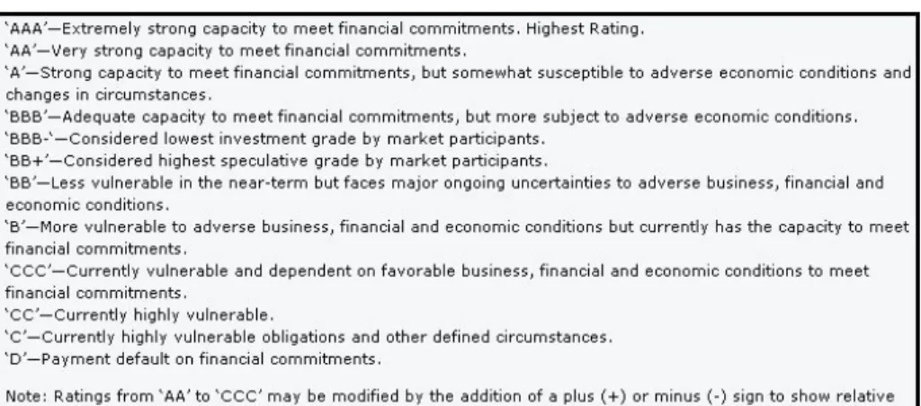
A credit rating agency is a company that issues ratings for dierent kind of loans. The ratings are meant to show what credit quality an investor can expect from dierent obligors. Most rating agencies uses some kind of letter combination for dierent ratings, e.g. AAA for an obligor with a very small estimated probability of default. See g 2.1 for an example.

(10)

Figure 2.1: Rating classes from Standard & Poor's. Source: www.standardandpoors.com.

To decide what rating to give an obligor, the rating agencies consider both qualitative and quantitative information about the obligor's economical situa-tion and tries to predict its future ability to repay debt. This informasitua-tion could be both hard gures, for example the obligor's current total debt, and facts that are more dicult to interpret, like the current political situation in the obligor's country. It is a dicult and exhaustive job to analyze all this information, therefore many investors use credit ratings issued by rating agencies instead of doing this analysis on their own.

The three by far most well-known and used credit agencies Fitch, Standard & Poor's and Moody's are all American, but there exists other smaller rating agencies from other parts of the world as well. Since so many investors use credit ratings from these three agencies, their ratings aect the market prices of bonds and other tradable debt. For example, an investor owning bonds issued by a large AA-rated country can at any time sell them at the bond market, assuming some liquidity on the bond market. However, if the country is downgraded to A-rating the market price is likely to instantly drop, reducing the present value of the investor's portfolio. The risk the investor faces by owning the bonds can be considered as credit risk.

Example 1. A simple model for credit risk could look as follows. A Swedish investor owns a bond issued by a British company. The company is B-rated by a rating agency that only uses four dierent rating classes: A, B, C and D for

default. The bond matures in three years and then pays the owner 100 GBP.

The current market price of the bond is86.38, which corresponds to a5%yield

since

100

1.053 = 86.38.

(11)

has a one-year-risk horizon. In one year the bond will have the market value

86.38·1.05 = 90.70. However, it is also assumed that an upgrade to rating A

gives an10%increase in market value, a downgrade to C a10%decrease and a

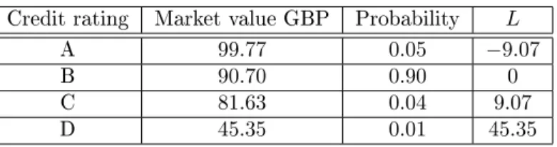
default gives a50%decrease resulting in the values in table 1. The probabilities

of these dierent states are assumed to be known as well.

Credit rating Market value GBP Probability L

A 99.77 0.05 −9.07

B 90.70 0.90 0

C 81.63 0.04 9.07

D 45.35 0.01 45.35

Table 1: Dierent scenarios for the bond one year from now.

Since it is in some sense expected that the bond will stay in rating class B,

the random variableLdescribing the credit loss in one year from now, is dened

as the dierence between the forward value given that the bond stays B-rated

and the actual forward value. This results in the dierent values ofLthat can

be seen in table 1. Also, the probability function ofLis shown in gure 2.2.

−200 −10 0 10 20 30 40 50 0.1 0.2 0.3 0.4 0.5 0.6 0.7 0.8 0.9 1

Loss distribution for the simple model

Losses in GBP

probability

Figure 2.2: The probability distribution ofL in example 1.

(12)

large probability of small or no loss and a small probability of a very large loss. Notice how the model tries to capture the credit risk in isolation. By holding the bond, the company in reality faces an interest risk as well, since the yield of the bond might change even without a credit rating change. Fixing the yield and subtracting from the forward value of a B-rated bond is an attempt to exclude the interest rate from the model. In the same way, if the company wanted to evaluate the risk in SEK instead, they could eliminate the currency risk from the model by xing the exchange rate.

2.2 Risk measures

In order to quantify the credit risk in a portfolio it is common practice to use risk measures. To get the full picture of what the risk structure looks like, it is of course best to study the full probability density function of the loss

L. However, this may be inconvenient if one for example wants to compare

two dierent portfolios. If it is possible to nd a single number that in an appropriate way describes how big the risk is, it would be possible for a bank to analyze time series of how the risk in the portfolio changes, make policies about how big risks that are acceptable and to minimize the risk given some constraints. In the following sections some commonly used risk measures will be presented. A reference for risk measures is (Dowd, 2002, pp. 27-44), which

especially introduces and discussesV aRandES. ELandU Lare pretty straight

forward, but are also dened in (van der Hoorn, 2009, pp. 125-128). 2.2.1 Expected Loss

Expected loss (EL) is simply dened as the expected value of the lossL, i.e.

EL=E[L].

ELis a very basic measure of risk and has some obvious drawbacks since it does

not say anything about the diusion ofL. However, for risk-neutral investors,

portfolios with the sameEL are considered equal. Theoretically, any rational

investor without any other information about the loss distribution would always

prefer the one with the lowestEL. In reality, however, investors are known to

be risk-averse, i.e. they do not want to risk loosing money unless they are

compensated for it. For example, a bank would in general not lend 100 USD

with a25%interest rate if the probability of getting the money back is0.8, even

though

EL= 0.8·(−25) + 0.2·100 = 0.

To accept giving the loan at all the bank would demand a higher interest rate. However, in a situation where the bank has a choice between two dierent borrowers with equal probability of paying back the loan, the bank will always choose the one which gives the best interest rate, or equivalently, the lowest

EL. This illustrates in what wayELcan be used as a risk measure. If two loss

distributions are known to be otherwise more or less similar, the one preferred

(13)

2.2.2 Unexpected Loss

Unexpected Loss (U L) is dened as the standard deviation of L. U L is

com-monly used in risk management to show the diusion of the distribution. For

risk-averse investors,U Lis of course preferred low. U Lis a good measure when

the loss distribution is light-tailed or approximately Gaussian (of course, when

the distribution is perfectly Gaussian,ELandU Ldescribes the distribution

en-tirely). Unfortunately, for credit risk the loss distribution is often heavy-tailed

since defaults often imply large losses. Therefore,U Lworks less well for credit

risk than it does for many other kinds of risk. 2.2.3 Value-at-Risk

Value-at-Risk (V aRα) is a widely used risk measure that focuses on the highest

percentiles of the loss distribution. It can be dened as

V aRα=min{l:P(L > l)≤1−α}, (2.1)

where α usually represents a large part of the probability mass and typical

values are α = 0.95 or α = 0.99. The idea behind Value-at-Risk is that it

should show a worst-case scenario, e.g. V aR0.99 could be interpreted as the

amount of money that the loss will only exceed in one year out of a hundred, in

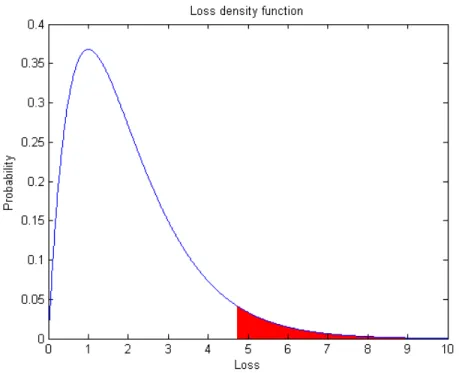
the long run. See g 2.3 for a graphical example. If the probability densityfL(l)

ofLis continuous and6= 0 on one interval only, then a more easily-interpreted

denition ofV aRα can be used

V aRα={l:P(L > l) = 1−α}.

I will sometimes in this paper, somewhat sloppy, use this denition even when the distribution is discrete to simplify my reasoning.

(14)

Figure 2.3: This graph shows an example of a loss density. The red section

represents5%of the total area. Thus,V aR0.95= 4.74.

A big reason to why V aR has become so popular is that it is in general

easy for everybody in an organization to understand the concept, as compared

to U L. It can also be argued that V aR tells more about the tail than U L

does. However, there are some well-known problems with usingV aR as a

risk-measure. For example, it is dicult to chooseαin a way that both shows how

large the losses could be in a very extreme case and how large they would be on

just a bad day. For this reason it is common to look atV aRfor manyα:s at the

same time. Another problem withV aRis that it does not satisfy sub-additivity,

i.e. for two random variablesL1 andL2

V aRα(L1+L2)≤V aRα(L1) +V aRα(L2)

does not hold in general (Dowd, 2002, p. 34). This is a problem since it contradicts the intuition that diversication, i.e. to hold many dierent assets,

lowers the risk. When optimizing a portfolio in terms ofV aR, the properties of

V aRcould lead to absurdities, which can be illustrated with an example.

Example 2. Consider two assets with loss distributionsL1andL2. L1takes the

value0with probability0.95and the value1000with probability0.05. L2takes

the value900 with probability0.991 and the value 109 _{with probability}₀_.₀₀₉_.

(15)

andV aR0.99(L2) = 900, so V ar0.99(L1)> V ar0.99(L2). This extreme example

shows thatV aRcan lead to absurdity as a risk measure.

2.2.4 Expected Shortfall

Expected Shortfall (ES) is a risk measure that tries to x the drawbacks with

V aR. ES is known by many names in the risk literature, with Expected

Tail-Loss, Conditional VaR and Tail VaR being the most common ones. The deni-tion looks as follows

ESα=E[L|L > V aRα].

So, while the denition ofV aR0.99could be interpreted as the amount that the

loss will exceed on average in only one year out of a hundred, ES0.99 can be

interpreted as the expected value of the loss in those worst1%years. For the

loss density in gure 2.3, ES0.95 is calculated as the center of mass of the red

section, i.e. ES0.95= 1 0.05· ∞ ˆ V aR0.95 l·fL(l)dl= 5.92,

where fL(l)is the probability density. Unlike for V aR, sub-additivity always

holds forES (Dowd, 2002, p. 37). Moreover,ES can handle cases like the one

in example 2 in a better way, since the whole tail aects its value. The problem

with choosing a goodα still remains, but is perhaps made somewhat smaller,

sinceES is always aected by the outermost part of the tail.

3 Monte Carlo methods

Monte Carlo methods is used in statistics in order to make calculations. The basic idea is to use a mathematical model for a phenomenon that appears ran-dom in order to make simulations. If the simulations are easy to generate, then one can produce a large sample and use the law of large numbers to approxi-mate for example the expected value of some process. Monte Carlo simulations works best, compared to other methods, when working with complex models of high dimension, since it may then be dicult to calculate things analytically or even numerically with deterministic methods. An introduction to Monte Carlo methods can be found in (Sköld, 2006).

In credit risk, when working with a portfolio of risky assets, the dimension is usually high and Monte Carlo simulations are therefore very useful. For now, set aside the underlying model and just consider the case when it is possible to

generate samples from the random loss variableL. LetNbe the number of

sam-ples generated and letL1, L2, . . . , LN be the generated samples. An estimate of

ELcan then be calculated as the mean, i.e.

d EL= ¯L= 1 N N X i=1 Li.

(16)

The estimate is unbiased and by the law of large numbers dEL → E[L] as

N → ∞.The central limit theorem makes it possible to construct a condence

interval for a givenN. Since

√

NELd−E[L]

∼N 0, σ2(L)

for largeN a two-sidedq-condence interval forELcan be constructed as

d EL−λq/2 σ(L) √ N ,ELd+λq/2 σ(L) √ N , (3.1)

whereλq/2denotes the theq/2-quantile of the standard normal distribution and

whereσ2₍_L₎_{can be approximated by}

σ2(L)≈ 1 N−1 N X i=1 Li−L¯ 2 . (3.2)

Now, instead assume thatELis known. In this caseU Lcan be estimated with

basically the same method. LetXi= (Li−EL)2,i= 1, . . . , N. Then

[ V[L] = ¯X= 1 N N X i=1 Xi

is an unbiased estimator of the variance ofLsince

EhV[[L]i=E " 1 N N X i=1 Xi # = 1 N N X i=1 E[(Li−EL)2] =V[L].

Thus, an estimate of the variance of L is available and a condence interval

can be constructed in the same way as for EL. Since U L is dened as the

standard deviation ofL, taking the square root of this estimate and the

con-dence bounds will give an estimate and a concon-dence interval forU L. Of course,

another estimate ofU Lis given by the square root of (3.2), but the method I

present here makes it easier to construct a condence interval.

To get an estimate ofV aRα, rst order the simulated samples. LetL(1), L(2), . . . , L(N)

denote the ordered samples, such thatL(1) ≤L(2) ≤ · · · ≤L(N). The denition

of V aRα (2.1) suggests that a good estimate should be the smallest value l

such that at most1−αof the samples are larger thanl. Using the empirical

distribution function b FL(l) = 1 N N X i=1 1{Li<l} (3.3)

as an approximation of the true loss distribution function would imply that the

estimate should beV aR\α=L(dαNe)(usingd.eas a notation for rounding to the

(17)

way to construct a condence interval forV aRα is presented in (Gupton et al.,

1997, pp. 150-151). The method is based on the binomial distribution. Given

the true value of V aRα, the random variable Y representing the number of

samples larger than V aRα is binomially distributed, i.e. Y ∈ Bin(N,1−a).

Notice, that for some integersA, B, such that,0< A≤B < N the event

A≤Y ≤B

is exactly the same event as

L(N−B)< V aRα< L(N+1−A).

For example, if it is known that the number of simulated samples that exceed

V aRα is greater than or equal to 3, but smaller than or equal to6, then one

knows that third largest sample must greater thanV aRα and that the seventh

largest sample must be smaller than V aRα and vice versa. Because of this, a

condence interval forY gives condence interval forV aRαas well. IfNis fairly

large andαis not too close to one (rule of thumb: ifN α(1−α)>10(Blom et al.,

2005)) a normal approximation can be used forY, i.e. Y ∼N(N α, N α(1−α)).

Aq-condence interval forY is thus

N α−λq/2 p N α(1−α), N α+λq/2 p N α(1−α)

and an interval forV aRαcan be constructed as

L bN−N α+λq/2 √ N α(1−α)c, LdN+1−N α−λq/2 √ N α(1−α)e ,

where the rounding has been chosen to make the interval as large as possible.

This bias will decrease asN increases.

For estimating ESα we can use the fact that we already have an estimate of

V aRα. If we insertV aR\αinto the denition ofESαwe see thatESαis the

ex-pected value of losses greater thatV aR\α. Thus, we can use the ordered samples

to get the estimate as d ESα= 1 N− dαNe N X i=dαNe+1 L(i)

, i.e. as the mean of the losses greater thanV aR\α. In the same way a condence

interval forESα can be constructed by taking the mean of losses greater than

the condence bounds forV aRα. Another, equivalent way of estimating ESα

is as d ESα=V aR\α+ 1 (1−α)N N X i=1 max(Li−V aR\α,0), (3.4)

(18)

which does not need the samples to be ordered. To show why this estimator works we consider the distribution function

FL|L>x(l) =P(L≤l|L > x) =

P(x < L≤l) P(L > x) =

FL(l)−FL(x) P(L > x) .

Taking the derivative of both sides gives

fL|L>x(l) = fL(l) P(L > x). Now E[L|L > x] = ˆ ∞ x l·fL|L>x(l)dl= 1 P(L > x) ˆ ∞ x l·fL(l)dl= 1 P(L > x) ˆ ∞ x (l+x−x)·fL(l)dl= 1 P(L > x) xP(L > x) + ˆ ∞ x (l−x)·fL(l)dl = x+ 1 P(L > x) ˆ ∞ 0 max(l−x,0)·fL(l)dl=x+ 1 P(L > x)E[max(L−x,0)].

Insertingx=V aRα on both sides nally gives

E[L|L > V aRα] =V aRα+ 1 P(L > V aRα) E[max(L−V aRα,0)] ⇔ESα=V aRα+ 1 1−αE[max(L−V aRα,0)], (3.5)

which explains the estimator in (3.4). We will return to this estimator in section 6 on optimization.

3.1 Importance sampling

Importance sampling (IS) is used in Monte Carlo methods as a so called variance reduction technique. The idea behind IS is that some possible outcomes of the random variable might be more important for the estimation than others and to make sure that these outcomes are included in the samples one can tweak their probabilities. For example, in credit risk there is typically a small chance

of very large losses. As the estimates of V aRand ES depend strongly on the

largest outcomes of the simulation these estimates can vary a lot depending on if the simulated sample contains many or few of these largest outcomes. Since the probability of the largest losses is typically very small, the estimators will have a large variance.

With IS the probability densityfL(l)ofLis replaced by an instrumental

distri-butiongL(l)that will typically increase the probability of the more important

outcomes. To be able to get correct estimates using the instrumental distri-bution, the estimators presented in the last section will have to be changed

(19)

to compensate for this. When calculating the expected value of an arbitrary

functionφ(L)we used in the last section that

E[φ(L)] = ˆ φ(l)fL(l)dl≈ 1 N N X i=1 φ(Li),

where Li are the simulated samples from fL(l). Now, when instead using the

instrumental distribution for simulating we can use that

E[φ(L)] = ˆ φ(l)fL(l)dl= ˆ φ(l)fL(l) gL(l) gL(l)dl= ˆ φ(l)ω(l)gL(l)dl≈ 1 N N X i=1 φ(Li)ω(Li),

where Li is now simulated using gL(l) and ω(l) = f_gL(l)

L(l) is called the

weight-ing function. This gives us a way to make estimations usweight-ing the instrumental

distributiongL(l), using the weighting function of each sample as a way to

com-pensate for its new probability.

ELcan now be estimated as

d ELIS = 1 N N X i=1 Liω(Li).

A condence interval can also be constructed similarly to that in the standard

case. The only dierence is that the estimate ofσin (3.1) is replaced by

σ2≈ 1 N−1 N X i=1  Liω(Li)− 1 N N X j=1 Ljω(Lj)   2 .

For the importance sampling to be meaningful this new estimate ofσshould be

lower than the old one. This will maybe not be the case when estimatingEL

becauseELdoes not depend that much on the tail events, but it will be for the

other risk measures. Assuming as before thatEL is now known, we can also

make an estimate ofU Las d U LIS = v u u t 1 N N X i=1 (Li−EL)2ω(Li)

and construct a condence interval similarly to before.

To get an estimate ofV aRαI will take a slightly dierent approach sinceV aRα

is not dened as an expectation of a function ofL, but a rather as a percentile

to the probability densityfL(l). Assume now thatV aRα is known but that α

is unknown. We could then get an estimate ofαusing that

α=P(L < V aRα) =E

1{L<V aRα}

(20)

so ˆ α= 1 N N X i=1 1{Li<V aRα}ω(Li)

is an unbiased estimate of α. Now, again assume that α is known and that

V aRαis not. If we could nd a numberV aR0αs.t.

ˆ α0₌ 1 N N X i=1 1{Li<V aR0α}ω(Li)≈α,

V aR0α should be a pretty good estimate ofV aRα. A way to nd such a

num-ber V aR0α is the following. Order the samples L1, . . . , LN like in the last

sec-tion to obtain the ordered sampleL(1), . . . , L(N). By summing up the weights

ω(L(1)), . . . , ω(L(N))in reverse order we can nd a numberk s.t.

1 N N X i=k+1 ω(L(i))≤1−α, but 1 N N X i=k ω(L(i))>1−α.

By comparing with the denition ofV aRit can be argued thatV aR\α

IS =L(k)

will be a good estimator. This method of course requires that 1

N

PN

i=1ω(L(i))>

1−α. To construct a condence interval forV aRα when using IS I will use the

same reasoning as in the standard case. However, in this case we do not know

the probability of a simulated sample being larger thanV aR\α

IS

, but the best

estimate is naturally N−k

N . Therefore I letY ∈Bin(N,

N−k

N )and proceed as in

the standard case.

For ESα we once again use that we have already estimated V aRα and use

(3.5), which gives the estimator d ESα IS =V aR\α IS + 1 1−α 1 N N X i=1 max(Li−V aR\α IS ,0)ω(Li) = \ V aRα IS + 1 1−α 1 N N X i=k+1 (L(i)−V aR\α IS )ω(L(i)).

The condence interval forESαcan be constructed in a similar way, using the

(21)

4 Modeling

I will in this section introduce a portfolio model for credit risk. The model is very similar to one that ECB has used, presented in (van der Hoorn, 2009). This itself is clearly based on the framework model CreditMetrics, presented in (Gupton et al., 1997). I start by explaining how the model works for a single bond. This is then extended to a model for a portfolio of bonds. I show how the dierent risk measures can be calculated and nally, I discuss how the dierent parameters of the model could be handled and estimated.

The main purpose of the model is to provide a way to make estimates of the dierent risk measures presented in section 2.2. This is mainly done by using Monte Carlo simulations, since the model provides a simple way to generate

random portfolio credit losses from the loss distribution FL(l). These

simula-tions can of course also be used to get a picture of what the wholeFL(l)looks

like using the approximation FbL(l), dened in (3.3). In section 6 we will also

see how the model can be used for minimizing the risk.

4.1 One-dimensional model

If the portfolio consists of only one bond or bonds from a single obligor, the model will be one-dimensional. In this case the model will be much simpler since the joint probability functions of dierent bonds do not have to be con-sidered. The one-dimensional model will in fact be very similar to the model described in example 1. For the model to work there must exist a rating system

that links every obligor with a certain rating. In the ECB-model9dierent

rat-ing classes is used, but in the model I have implemented I have used18dierent

rating classes from AAA to D and the ratings has been taken from Fitch1_{. The}

number of rating classes does not matter for the explanation of the model and

it is unclear how it eects the performance as well. The reason why I use18

is mainly a practical matter of data availability. Sometimes the ratings will be

referred to as numbers rather than letters in their natural order, i.e. AAA= 1,

AA+= 2,. . ., D= 18.

As mentioned before the risk horizon considered will be one year. The model could be generalized to work for dierent time horizons as well, but this will lie outside the scope of this paper. One of the most important parameters for the model will therefore be the probabilities of rating changes for dierent obligors in one year's time. A fundamental assumption will be that obligors that have the same rating today will have the same probability of a rating change to a given rating in one year's time. These probabilities can therefore be presented in a so called migration matrix. Migration is just another word for rating change.

If the number of dierent ratings isrthe size of the migration matrixM will be

r×rand on position(i, j)the matrix will contain the probability that an obligor

1_{The complete list of ratings is} AAA,AA+,AA,AA-,A+,A,A-,BBB+,BBB,BBB-,BB+,BB,BB-,B+,B,B-,C,D.

(22)

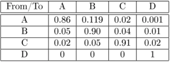
of ratingi migrates to ratingj in one year's time. An example of a migration

matrix can be seen in table 2. In practice migration matrices is usually based o n historical data, which will be described in section 4.4.1.

From/To A B C D

A 0.86 0.119 0.02 0.001

B 0.05 0.90 0.04 0.01

C 0.02 0.05 0.91 0.02

D 0 0 0 1

Table 2: A ctional migration matrix with4rating classes. Every row contains

the probabilities of migration to the rating classes represented by the columns.

For example, the probability of an obligor upgrading from C to A is2%and the

probability of a B-rated obligor moving into default is1%.

In addition to assuming that obligors with the same rating have the same probabilities of migration it will also be assumed that they are associated with the same yield. This means that all future cash ows coming from bonds issued by the same obligor will be discounted using the same discount factor. The

discount factor used for an obligor with rating i will be denoted dfi. Now,

suppose that we have a portfolio containing bonds issued by a single obligor

with ratingioldand that we will receive cash ows at timest1, t2, . . . , tkof sizes

CF1, CF2, . . . , CFk. Then the value of the portfolio one year from now will be

F V = k X j=1 dfiold tj−1_CF j,

assuming that the obligor's rating does not change and thattj ≥1 for all i. In

the same way, if the obligors rating changes toi, the new value will be

k

X

j=1

dfitj−1CFj.

If the obligor defaults no future cash ows will be received, but we instead

assume a constant recovery rateRR, so that the new value will beF V·RR. We

are now ready to dene the conditional credit lossCLi given a rating change as

CLi=

(

F V −Pk

j=1dfitj−1CFj if i6=D

F V(1−RR) if i=D. (4.1)

Lcan thus be seen as a random variable that takes the valuesCL1, CL2, . . . , CLr

with probabilities from the migrations matrix, i.e. M(iold,1), M(iold,2), . . . , M(iold, r).

(23)

to calculate the risk measuresEL,U L,V aR andELanalytically. For example, EL = r X τ=1 M(iold, τ)·CLτ U L = v u u t r X τ=1 M(iold, τ)·(CLτ−EL) 2 . (4.2)

4.2 Multi-dimensional model

The issue when moving from the one obligor portfolio to a portfolio consist-ing of many obligors is how to model the joint distribution of ratconsist-ing changes, while keeping the marginal distributions for single obligors equal to the one-dimensional model. One cannot assume that the migrations of dierent obligors are independent since it is presumable that countries that are strongly linked economically will have a similar economical situation and will hence move simi-larly in credit ratings. That this is the case for corporations is shown empirically by Gupton et al. (1997, pp. 81-83), where they estimate condence intervals for default correlations among rms, which do not cover zero.

Instead, a model in the fashion of the classical model by Merton (1974) will be used. The idea is that for every obligor there exist an underlying

Gaus-sian random variableZ. If the obligor is a company, Z could be thought of as

the total value of all the company's assets one year in the future. In my case, where the portfolio consists of obligors that are sovereign states, the

interpre-tation ofZ is not that simple. It may however be thought of in a similar way

as the amount of money the state could make available in the near future. It

is also assumed that there exists some x numbers qD, qC, . . . , qAA+ such that

qD≤qC≤ · · · ≤qAA+. These numbers are meant to represent certain levels of

debt that corresponds to the dierent rating classes. Especially,qD represents

the total value of the payments that the obligor has to make one year from now.

If the obligor is unable to make the payments, i.e. if Z < qD, the obligor will

default. In the same way, qD ≤ Z < qC means that the obligor gets rating

C, qC ≤ Z < qB− means that the obligor gets rating B- etc. However, we

already know the probabilities of these events from the migration matrix. So,

if the obligor has rating i these probabilities, for theZ linked to that obligor,

would be P(qAA+ ≤Z) = M(i,1), P(qAA≤Z < qAA+) = M(i,2), . . . , P(Z <

qD) =M(i,18). Now, given the migration matrix the relationship between Z

andqD, . . . , qAA+ is xed soZ can be normalized to a standard Gaussian

vari-able, i.e. Z ∈N(0,1)and then (the normalized version of)qD, . . . , qAA+can be

(24)

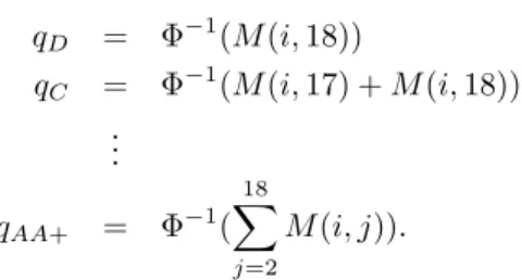
function then qD = Φ−1(M(i,18)) qC = Φ−1(M(i,17) +M(i,18)) ... qAA+ = Φ−1( 18 X j=2 M(i, j)).

This implies thatqD, . . . , qAA+will be the same for obligors of identical ratings.

The relationship ofM,Z and theq:s is visualized in g 4.1. Now, a new matrix

Qcan be constructed. Qwill have sizer×r−1and each row will contain the

valuesqD, . . . , qAA+corresponding to the dierent initial ratings.

−4 −2 0 2 4 0 0.05 0.1 0.15 0.2 0.25 0.3 0.35 0.4 B q D D q B q C A C

Figure 4.1: This graph shows the probability density of Z together with the

valuesqD, qC, qB derived using the second row in the ctional migration matrix

M in table 2. The areas under the graph named A, B, C and D have sizes equal

to the probabilitiesM(2,1), M(2,2), M(2,3)andM(2,4). For a B-rated obligor

the rating one year in the future can thus be decided by comparing the outcome

ofZ to the dierentq:s. For example, the eventqD ≤Z < qC is equivalent to

the obligor being downgraded to C.

Using the model with underlying Gaussians we can now construct the

(25)

multivariate Gaussian vector ¯ Z=      Z1 Z2 ... Zn      ,

whereZ1, . . . , Zn are the underlying Gaussians linked to obligor1, . . . , n. Since

allZ1, . . . , Zn are standard Gaussians they all have mean0and variance1, but

we introduce the covariance matrix

Σ =      1 ρ1,2 · · · ρ1,n ρ2,1 1 · · · ρ2,n ... ... ... ... ρn,1 ρn,2 · · · 1      ,

where ρi,j is the correlation between Zi and Zj implying that ρi,j =ρj,i and

−1 < ρi,j <1 for all i 6=j. The dierentρ:s will be input parameters to the

model and how to estimate them will be discussed in section 4.4.3.

The underlying multivariate variable_Z¯_{describes the joint distribution of rating}

changes completely and the credit lossLfor the n-obligor portfolio can now be

dened as L= n X i=1 Li,

whereLinow denotes the credit loss from obligori, dened as in one-dimensional

model. While it was fairly simple to compute the probability functionpL(l)of

L for the one-dimensional model, for the multi-dimensional model it quickly

becomes computationally impossible asngrows. The Riksbank's portfolio

typ-ically consists ofn= 30 obligors. Using the system withr= 18 rating classes

implies that there is a total of rn = 1830 ≈ 5·1047 combinations of rating

changes for the dierent obligors. To calculate the probability of each of these outcomes one has to integrate the multivariate Gaussian density function over

ann-dimensional rectangle. For example, to calculate the probability that all

obligors default one must integrate over the rectangle with corners in      −∞ −∞ ... −∞      ,      qD,1 qD,2 ... qD,n      ,

where qD,1, etc. are theqD:s associated with the ranking of obligor 1 etc. A

quick test in Matlab using the built-in function mvncdf and n= 25 (which is

the highest dimension that the Matlab function allows) shows that each such

integration takes approximately0.3 seconds. Needless to say, calculatingpL(l)

(26)

4.3 Calculating risk measures

We saw in the last section that it was very hard to obtain the probability

func-tion of the credit loss Lexactly as the dimension of the model became larger.

One can however say much about the credit risk just by examining the risk

measures EL,U L,V aR and ES. In this section I will show how these can be

calculated. EL andU L can be calculated exactly analytically and all of them

can be approximated using Monte Carlo methods. The Monte Carlo method

will give an approximation ofpL(l)as well.

To calculate EL is very simple since the joint distribution of rating changes

does not matter. We have

EL=E[L] =E[ n X i=1 Li] = n X i=1 E[Li],

where E[Li] is the expected loss from obligor i, calculated as in (4.2). To

calculateU Lis a little trickier and more time consuming, but can be performed

in acceptable time. U Lis computed aspV ar[L]. We have that

V ar[L] =V ar[ n X i=1 Li] = n X i=1 V ar[Li] + 2 X i<j Cov[Li, Lj].

Here eachV ar[Li]can be obtained as the square ofU Lin (4.2). In the second

termCov[Li, Lj]can be calculated by rst computing the joint loss probability

function for the corresponding two-obligor portfolio, let us call itpL0_,L00(u.v).

ThenE[Li·Lj]can be calculated as

E[Li·Lj] = r X u=1 r X v=1 uvpL0_,L00(u.v)

andCov[Li, Lj] =E[Li·Lj]−E[Li]E[Lj]. To get everypL0_,L00(u.v)one must

dor2 _{integrations over a bivariate normal density and there will be} n(n-1)

2

co-variances to calculate resulting in n(n_-1)

2 r

2 _{integrations in total. For the typical}

caser= 18, n= 30this gives≈105_{integrations in total. A Matlab test shows}

that each integration takes approximately0.006 seconds in the bivariate case,

so calculatingU Lfor the whole portfolio would take something like600 s= 10

minutes. This shows that U L is denitely computable analytically, but using

Monte Carlo methods will be much faster and accurate enough so that is the method that I will use from now on.

To use the Monte Carlo methods explained in section 3, one needs to be able to generate pseudo-random samples from of the portfolio credit loss variable

L. This can be done by rst simulating the multivariate Gaussian vector Z¯

of underlying variables. This can be done for arbitrary mean and covariance matrix with the Matlab function mvnrnd. I will not go into detail how this

(27)

is done mathematically, but it involves a Cholesky factorization of the

covari-ance matrix Σand is explained in (van der Hoorn, 2009, pp. 130-131). Once

¯

Z is simulated each Zi can be compared to the adequate row in the matrixQ

that corresponds to that obligors current rating. This way one gets the rating changes of all obligors in the portfolio and the credit loss for each obligor can

be obtained. Summing them up gives L. To make the simulation fast I have

noticed that it is advantageous to rst guess that each obligor will stay in

the same rating class, when comparing the values in_Z¯ _{to those in} _Q_{. This is}

because there is usually a high probability for the obligors staying, so making this guess reduces the number of comparisons.

A test on my computer shows that each sample from L takes approximately

2.5·10−6_{seconds to generate when}_n_{= 29}_{, so a million samples or so can easily}

be generated. Now, when it is possible to generate such a large sample fromL,

the methods in section 3 can successfully be used to give good approximations of the risk measures. An approximation of the probability function can also be constructed as ˆ pL(l) = 1 N N X i=1 1{l=Li},

whereN is the number of samples (this is more or less equivalent to the EDF

dened in (3.3)). The probability function can be visualized by plotting a his-togram of the samples, for results see section 5.

Usually the probabilities of downgrade or default for obligors are very low. Therefore the probability function will naturally look skew with a fat tail, like

in example 1. The risk measures V aR and EL that depend mostly on the

tail of the distribution are therefore sensitive to the largest samples from the simulation. Since the worst outcomes will occur very seldom even in a million

samples, this will result in a high variance for the estimates ofV aR and EL

and large condence intervals. The variance can be decreased by the use of importance sampling as explained in section 3.1. For IS to work we need to

nd an instrumental distributiongL(l)that will simulate the larger losses with

a higher probability. This can be done in a number of ways, but the method

I will use is to change the mean for the underlying variable_Z¯_{. Originally the}

meanµ_Z¯ = ¯0, but since low outcomes for the elements inZ¯ implies downgrades

we can increase the probability of downgrades in the simulation by lowering the

mean of _Z¯_{. How much the mean should be lowered for the dierent obligors}

to get a high variance reduction depends on the probabilities in the migration

matrix. If we denote the original density function of_Z¯_,_f_¯

Z and the new onegZ¯,

then we can construct the weighting functionωneeded for the IS estimators as

ω(L) =fZ¯( ¯Z) gZ¯( ¯Z) .

Now we have everything we need to calculate the risk measures using importance

(28)

Since pL(l) =P(L=l) =E 1{l=Li} , then ˆ pIS_L (l) = 1 N N X i=1 1{l=Li}ω(Li).

4.4 Estimating parameters

So far in this section I have presented the model and showed how the dierent risk measures can be computed, given this model. However, for the model to be useful, we need a good way to estimate the parameters that the model is based upon. These parameters include the migration matrix, the conditional credit losses and the correlation matrix.

4.4.1 Migration matrix

The migration matrix M is supposed to contain the probabilities of obligors

being in the dierent rating classes in one year's time given their current rating classes. The most basic way of estimating this is of course to look at historical data and register how many migrations there has been between each combination of ratings every year. The rating agencies all provide these historical matrices, see g 4.2 for an example.

Figure 4.2: A migration matrix from Fitch simply reecting the average number of rating changes every year in the period 1995-2011 among the sovereign issuers that Fitch rates.

The matrix in g 4.2 is typical for the migration matrices that the rating agencies provide. It has a lot of zeroes, reecting that it is unusual for obligors to migrate more than one or two rating classes in one year. There are however

some exceptions, for example the1.72% that has moved from AA- to B-. The

reason to why the matrix looks like this is of course that the data is very limited. It has only been collected for 17 years and there are presumably not that many issuers in every rating class. To use this matrix directly in the model is probably

(29)

a bad idea and doing so gives very unrealistic results. I did a quick test with this matrix and some dierent ctional portfolios of the same value. The test

showed a much higher level of risk, in the sense ofV aRandES, for portfolios

that contained obligors with rating AA-, than for example portfolios containing obligors rated A-. This is very contradictory, since the whole idea behind the rating system is to show which obligors that are more risky.

To make the model more realistic I would like to change or re-estimate the matrix in some way. I have looked at a few options for this. In the ECB model presented in (van der Hoorn, 2009) they do this by only focusing on the probability of default (PD) for every rating class. Since the default state gives the biggest losses this is the most important to change and they argue that even if it there are no observed defaults for the highest ratings, it could happen and therefore the probabilities in the last column should be positive and in as-cending order. Hence, they assign positive PD:s for all initial rankings. What probabilities to use seems mainly subjective, but they try to use something that seems reasonable. For example they let the PD for AAA-rated obligors be

0.01%, for AA-rated0.04%and so on. To make sure every row sums to one they

lower the probabilities on the diagonal. This method is very ad hoc, but may generate results that seem more reasonable than when using the original matrix. In (Gupton et al., 1997) they mention some properties that are desirable for a migration matrix, for example that better ratings never should have a higher chance of default or downgrade to a certain rating and that the chance of mi-grating to a given rating should be greater for more closely adjacent rating categories. They then try to nd a best t in some least squares sense to the original migration matrix, while keeping these constraints fullled. In addition to tting to the original matrix they also try to make it t some other data, for example historical migration averages for longer time periods than one year by

assuming Markov properties, i.e. that the migration matrix fornyears should

be equal to Mn. They do not say exactly what method they use for nding

the least squares t, but I try to do something similar to their method using the build in Matlab function lsqnonlin. I use three dierent migration matrices as input, corresponding to one, three and ten years migration times. Unfortu-nately, I nd it very hard to make the method robust and at the same time keep every probability greater than zero, guarantee that every row has sum one, etc. Instead, I try something dierent, inspired by the method that we used to construct the multi-dimensional model, with the underlying Gaussian variables.

Recall that underlying variableZ could be thought of as the total value of the

obligors assets and qD, . . . , qAA+ as some xed levels of debt. When we

con-structed the multi-dimensional model we let allZ:s be standard normal and the

q:s be dierent for every initial rating. Now, instead assume that there only

exist one set ofqD, . . . , qAA+and that there exists dierentZ:s for every initial

(30)

dierent meanµAAA, . . . , µC and that all have the same variance σ2= 1, s.t. qD≤µC< qC≤µB− <· · · ≤µAA+< qAA+≤µAAA. (4.3)

This assumption would be consistent with their current rating. I x qD = 0,

otherwise translating all theq:s andµ:s an equal distance would just result in

the same thing. My idea is now to try to ndq:s andµ:s s.t. the probabilities

of the Z:s migrating to the dierent rating classes match the probabilities in

the historical migration matrix. Given all the q:s and µ:s the probability of

migration from one rating class to any other can be calculated. For example, the the probability of migration from BBB to B+ is

P(qB≤ZBBB < qB+) =FZBBB(qB+)−FZBBB(qB).

These probabilities can then be used to construct a new, re-estimated migration matrix. This method will have the benet of keeping every row sum in the matrix equal to one and as well every element strictly greater than zero. In addition some order relations will automatically be fullled, for example that the probability of default is lower for better ratings. Unfortunately, Fitch does not include what number of obligors that has been used to calculate each percentage in the historical migration matrix. If this had been the case it would have been possible to treat the historical migration matrix as pure data and I could probably had come up with some Maximum Likelihood estimator, given this

model. I would then nd theq:s and µ:s that were most likely to generate the

data.

Now, I will instead use a least squares method that minimizes the sum of the squared dierences between each element in the historical migration matrix

and each element in the migration matrix implied by theq:s andµ:s (except the

last row). I use the built in Matlab function lsqnonlin, and as starting values

I useµC = 0.5, qC = 1, µB− = 1.5, qB− = 2. . . and so on. To make sure that

the order condition (4.3) is fullled I add an extra penalty to the function if it is not. The function runs in a few seconds. A numerical test of this method is presented in the following example.

Example 3. In this example I will use a historical migration matrix from Fitch with only eight dierent rating classes to make it easier to look at the result. The least squares method is used to estimate a new migration matrix. The results are presented in table 3.

(31)

From/To AAA AA A BBB BB B C D AAA 0.9862 0.0138 0 0 0 0 0 0 AA 0.0379 0.9242 0.0273 0.0095 0 0.0047 0 0 A 0 0.0273 0.9235 0.0437 0.0055 0 0 0 BBB 0 0 0.0631 0.8931 0.0340 0.0049 0.0049 0 BB 0 0 0 0.0939 0.8449 0.0490 0 0.0122 B 0 0 0 0 0.1000 0.8684 0.0263 0.0053 C 0 0 0 0 0 0.2500 0.5000 0.2500 D 0 0 0 0 0 0 0 1 From/To AAA AA A BBB BB B C D AAA 0.9862 0.0138 0.0000 0.0000 0.0000 0.0000 0.0000 0.0000 AA 0.0384 0.9375 0.0240 0.0000 0.0000 0.0000 0.0000 0.0000 A 0.0000 0.0275 0.9286 0.0439 0.0000 0.0000 0.0000 0.0000 BBB 0.0000 0.0000 0.0637 0.9019 0.0343 0.0000 0.0000 0.0000 BB 0.0000 0.0000 0.0000 0.0951 0.8553 0.0496 0.0000 0.0000 B 0.0000 0.0000 0.0000 0.0000 0.1004 0.8719 0.0272 0.0006 C 0.0000 0.0000 0.0000 0.0000 0.0001 0.2507 0.4985 0.2507 D 0 0 0 0 0 0 0 1 µC qC µB qB µBB qBB µBBB qBBB µA qA µAA qAA µAAA Starting value 0.5 1 1.5 2 2.5 3 3.5 4 4.5 5 5.5 6 6.5 Estimates 0.7 1.3 3.3 4.5 6.2 7.5 9.3 10.8 12.6 14.5 16.4 18.2 20.4

Table 3: Tables for example 3. The top table shows the historical migration matrix. The middle table shows the re-estimated migration matrix and the

bottom table shows the starting values and estimates of theq:s andµ:s.

As can be seen in the results from example 3, the new migration matrix is not very dierent from the old one. The biggest dierence is that the prob-ability to move from rating AA to rating B has been signicantly lowered as well as for some of the default probabilities and the probability mass has been moved towards the diagonal. I have tried this method for some other migration matrices as well and have got more or less the same result. Small probabilities outside of the main diagonal has been more or less erased. It is hard to say if the new matrix is more or less realistic than the old one. The new matrix does fulll order relations between ratings, but this has been done by basically eras-ing probabilities that violates it. The new matrix also has positive probabilities for every migration, but the ones that are far from the diagonal are so small

that they do not make any numerical dierence anyway2_{. One can also question}

how likely the observed historical migration matrix is given the new estimated one. One issue with this least squares method is that it treats all probability

2_{The PD for AAA-rated obligors in example 3 is even smaller than the smallest number} Matlab can handle≈10−325_{so it is treated as identically zero.}

(32)

dierences equally. If the historical matrix would for example show a0.1%PD

for AAA this would be a signicant risk factor, but the method would just erase this probability rather than raising the probabilities for downgrades. As a x to this I tried to come up with a way to weigh the elements of the matrix dierently in the least squares function, but I was not able to make much improvement. For the calculations below I will use the historical matrix in g 4.2. For

com-parison, I will also use the same matrix but with theP D:s tweaked in the same

way as in the ECB paper.

4.4.2 Conditional credit losses

The conditional credit loss (CLi) indicates how big the credit loss is for an

investment in a single obligorigiven the obligors rating one year from now. As

dened in (4.1), theCLi depends on four things:

The time points of the future cash ows (tj)

The sizes of those cash ows (CFj)

The discount factors (dfcr(i)) associated with the dierent credit ratings

The recovery rate (RR).

I have let cr(i) denote the credit rating of obligor i. The rst two points are

usually known exactly, since that is how bonds work. Every bond pays specied amounts on specied payment dates. For the Riksbank's portfolio, however, I have not been able to get hold of this information, probably because the portfolio is very big and contains a lot dierent bonds that are registered in

dierent systems, so it is a technical problem to get alltj and CFj in a single

list. Instead, I have been given the current total market value of each position

converted to SEK (T Vi) and the modied duration (M Di) of each position. The

M Diis the center of mass of the future cash ows along the time axis and could

be dened as M Di = P jCFjtj P jCFj .

Given the limitation of the data, I will instead view it as if there was only one

future cash ow from each obligor, having a size that equalsT Vi if discounted

bydfcr(i). Formally,

T Vi= (dfcr(i))M DiCFM Di,

whereCFM Di is the cash ow replacing the old ones.

The models assume that there exists a xed discount factor for every rating class that can be used to discount all future cash ows. Looking at market bond yield data one sees that this assumption is not perfectly true. The yield can vary quite much for countries in the same rating class and for dierent ma-turities. The yield can also be lower for lower rated countries, for example on

(33)

the 1st of July 2012 the yield for Japanese 10-year bonds was0.83% while the

corresponding value for French bonds was2.69%, even though France is rated

AAAand Japan is ratedA+by Fitch3. This is non-intuitive, but is a sign of

that the market cares about other things than Fitch's ratings and credit risk. However, this might not be such bad news for our model anyway, since we are mainly interested in the change of market value, when the ratings change. If France was downgraded to Japan's rating, we can be pretty sure that the yield would not decrease to the same yield as Japan, but instead increase due to the higher risk associated with the lower rating. Therefore, a good way to estimate the conditional credit losses might had been to look at how much the market value of dierent bonds has changed after rating changes, but I do not have that kind of data. Instead, I just choose dierent values for the dierent yields in an ad hoc way such that they reasonably match the current market yields of bonds from countries with the same rating and with maturities that are close

to the M D:s. Each discount factor is then calculated as one divided by the

corresponding yield.

For the recovery rates, there is very little data, since very few countries has defaulted during the last 15 years. The complete list can be seen in table 4. It is hard to come up with a single number for the recovery rate, based on this data. As can be seen the recovery rates varies a lot and the countries in this data set is generally of much lower rating than the ones in the Riksbank's portfolio.

For the model I use something in the middle, so I letRR= 0.55.

(34)

Year Defaulting Country Recovery rate (%) 1998 Russia 50 1999 Pakistan 65 1999 Ecuador 60 2000 Ukraine 60 2000 Ivory Coast NA 2001 Argentina 30 2002 Moldova 95 2003 Uruguay 85 2003 Nicaragua 50 2004 Grenada NA 2005 Dominican Republic 95 2006 Belize NA 2008 Seychelles NA 2008 Ecuador NA 2010 Jamaica 80 Issuer-Weighted RR 67 Value-Weighted RR 36

Table 4: Recovery rates on sovereign defaults during the last 15 years. The last two rows shows the average RR weighted per issuer and weighted by the total value of bonds respectively. Source: Moody's.

I now have everything needed to calculate the conditional credit losses. Since

there was some uncertainty in all the parameters used to calculate theCL:s it

will probably result in some model error and to make this part of the model

satisfactory, better data is needed. It will be important to update the CL:s

frequently as for example theM D:s change.

4.4.3 Correlations

The correlation between obligors' underlying assets is an important parame-ter for the risk measures, since a high correlation makes it more probable that countries get downgraded at the same time. These events will result in the largest portfolio losses. The correlations are typically positive, since countries usually react similar to changes in the world economy. There exist some known

methods to estimate the correlations in the correlation matrix Σ. In (Gupton

et al., 1997), which mainly focuses on corporate bond, they look at the com-panies' stocks time series to make an approximation of the comcom-panies' assets and estimate the correlation from this. They also group the companies into dierent groups, depending on sector and geographical location and estimate the correlations in the dierent group. They then come up with a clever way to base the correlation between two companies on the groupings.

(35)

technique. Countries do not issue stocks, so we cannot use that method to estimate the correlations. Maybe the method with groupings could be used, ex-ample by raising the correlation between countries in the euro zone, but we still need something to base the estimations on. The ECB approach is to just use

24%for all correlations, since this is suggested by Basel II4to be an upper limit

for the correlation. This method would result in estimates of the risk measures that will be more like upper limits of the risk measures.

I will try a dierent method for estimating the correlations, based on CDS spread data and inspired by Friewald (2009). A Credit Default Swap (CDS) is a credit derivative that works like an insurance against default. An illustration of the CDS contract can be seen in gure 4.3.

Figure 4.3: An illustration of how a CDS works.

For every CDS contract, there will exist a reference bond. The buyer of the

CDS contract, will pay an insurance ratesper year of the valueV of the bond

to the protection seller. If the issuer of the bond defaults, the protection seller pays the buyer an amount equal to the value of the bond and receives the bond in return, retrieving whatever the defaulted bond pays. In this way, in case of

a default the protection buyer reduces his losses byV(1−RR), where RR is

the recovery rate. CDS:s are quoted daily which means that there exists market

prices, quoted in the insurance rates. One can thus assume that the prices will

be fair. At least one can assume that the market is liquid enough to make prices for CDS:s on dierent bonds equally close to their fair price and since our main intention is to estimate correlations, this approximation should be adequate. If we assume a constant hazard rate, i.e. the probability of defaulting is the same at any time point in the next year, then a fair price of the CDS would be such

that the insurance rate s equals the hazard rate λ of the bond multiplied by

(1−RR), i.e.

λ= s

1−RR.

4_{Basel II are recommendations on banking laws and regulations issued by the Bank of} International Settlement.

(36)

Hence, the probability of default in one years time should be

P D= 1−exp(−λ·1) = 1−exp(− s

1−RR).

Given the recovery rateRR(we will assume as before thatRR= 0.55) we now

have a way of estimating the probability of default in one year's time based on the market CDS prices. The market CDS prices will of course only reect

investors' opinions on what theP Dis and not the trueP D itself, but this can

be seen as an approximation.

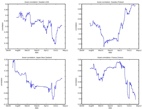
As input to this method I will use daily CDS prices from the time period 2008-2012 for 5-year bonds from some dierent countries. I denote the price of a CDS

si(t)for obligoriat timet. Similarly I denote theP Dfor the next year implied

by the CDS priceP Di(t). The prices are quoted about260times per year, so I

let the length of one day bed=₂₆₀1 andnd= 260. Now, recall the model with

the underlying process that we used to construct the multi-dimensional model. To be able to use the CDS data for estimating correlation I will for each obligor

idene an underlying processZi(t)by

Zi(t+d) =Zi(t) +εi(t+d),

whereεi(t)∈N(0, d)and independent fort=d,2d,3d, . . .. This impliesZi(t+

1)−Zi(t) =P nd

k=1εi(t+kd)∈N(0,1). I will as before assume that the exists

xed constantsqi

D for each obligor such that if the process is belowqiD a year

from now the obligor defaults. Thus ( P Zi(t+ 1)< qiD|si(t) =P Di(t) P Zi(t+d+ 1)< qDi |si(t+d) =P Di(t+d) ⇔ ( P Pnd k=1εi(t+kd)< qDi −Zi(t)|si(t) =P Di(t) PPnd+1 k=2 εi(t+kd)< qDi −Zi(t+d)|si(t+d) =P Di(t+d) ⇔ ( qi D−Zi(t) = Φ−1(P Di(t)) qi D−Zi(t+d) = Φ−1(P Di(t+d)) ⇒ Zi(t+d)−Zi(t) = Φ−1(P Di(t))−Φ−1(P Di(t+d)). (4.4)

By using (4.4), we have a method to estimate the increments of the underlying process. Using this method for dierent obligors will generate dierent processes which can be used to estimate the correlation between them. What we are

interested in is the correlationρbetween two assets over a one year time period.

ρ=corr(Zi(t+ 1)−Zi(t), Zj(t+ 1)−Zj(t)) =Cov(Zi(t+ 1)−Zi(t), Zj(t+ 1)−Zj(t)) = Cov nd X k=1 εi(t+kd), nd X k=1 εj(t+kd) ! = nd X k=1 Cov(εi(t+kd), εj(t+kd)) =ndCov(εi(t), εj(t))