to U.S. Economic Growth
2
Hye Mi Youa; y
a The State University of New York at Bu¤alo
Received Date; Received in Revised Form Date; Accepted Date
3
Abstract
4
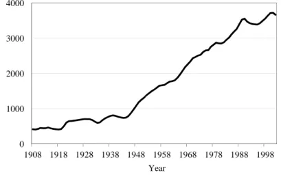
U.S. public school expenditures per pupil increased by a factor of 9 during the 20th century. This
5
paper quanti…es how much U.S. labor quality has grown due to the rise in educational spending. A
6
schooling model and cross-sectional earnings variations across cohorts are exploited to identify the
7
e¤ect of the increased school expenditures on labor quality growth. The …ndings are that (i) U.S.
8
labor quality increased by 0.4% per year between 1967 and 2000, one-…fth of which is attributable
9
to the rise in educational spending; and that (ii) labor quality growth explains one-quarter of the
10
rise in labor productivity.
11
Keywords: Labor Quality Growth, Rising School Quality, Growth Accounting
12
JEL classi…cation:E0, J24, O47
13
Corresponding author: Department of Economics, The State University of New York at Bu¤alo, Bu¤alo, NY 14260. Tel.: +1 716 645 8689. Email address: hyemiyou@bu¤alo.edu.
yI am deeply indebted to Mark Bils for his generous support and encouragement. For their valuable comments and helpful discussions, I thank Mark Aguiar, Yongsung Chang, Jay H. Hong, Byoung Hoon Seok, and seminar participants at the University of Rochester, the State University of New York at Bu¤alo, the Federal Reserve Bank of Richmond, Korea Development Institute, University of Western Ontario, Korea University, Far Eastern Meetings of the Econometric Society 2008, and Midwest Macro Meetings 2007. I would also like to thank the editor and an anonymous referee for their insightful comments and suggestions. All errors are mine.
1. Introduction
1
During the 20th century, the real spending per pupil in U.S. public elementary and 2
secondary schools increased by a factor of 9. This paper explores how much U.S. labor 3
quality has grown due to the rise in school expenditures. The Bureau of Labor Statistics 4
(BLS) currently measures labor quality growth mainly based on increases in the mean years 5
of schooling but fails to capture the impact of changes in the quality of education. If the 6
increased educational expenditures improved school quality, then the BLS underestimates 7
the growth in U.S. labor quality. 8
This paper proposes a new way of quantifying the rise in the quality of education with 9
a schooling model in which human capital production depends not only on time in school 10
but also on educational spending. This model as well as cross-sectional earnings variations 11
across cohorts is exploited to identify the growth in school quality. Consider cross-sectional 12
earnings di¤erences between younger and older cohorts with the same years of schooling. 13
The earnings variations re‡ect three components: i) the impact of changing selection into 14
di¤erent years of schooling; ii) return to experience; and iii) the growth in the quality of 15
education. Without a model, these three components cannot be identi…ed simultaneously. 16
To assess the e¤ect of the changing selection in schooling choice, assume that ability 17
distribution stays constant across cohorts. If years of schooling vary only by ability within 18
cohorts, the cohort-invariant ability distribution can be estimated by the schooling distri-19
bution of any single cohort. The impact of the changing selection on the cohort-variations 20
in earnings is then measured by accounting for changes in empirical schooling distribution 21
across cohorts. 22
Once the selection e¤ect is controlled for, a structural restriction derived from the model 23
is used to disentangle the remaining two components, assuming the same return to experience 24
across cohorts. In the model, optimizing agents choose both time in school and educational 25
expenditures so that their relative marginal product in increasing human capital equals 26
their relative costs. Given the data on individual earnings and educational expenditures, 1
foregone earnings due to delayed experience are the key element in the relative cost of time 2
spent in school. If earnings rise with work experience very rapidly, increasing time in school 3
is relatively more costly than raising educational expenditures. Thus, agents substitute 4
expenditure for time in school until the relative marginal product of expenditure equals its 5
low relative cost. According to the model, the relative marginal product of expenditure 6
for the last year in school equals the expenditure elasticity of human capital. Thus, the 7
low relative marginal product of expenditure represents a low value for the elasticity. This 8
implies little increase in the quality of education, given the rise in school expenditures. 9
By the same mechanism, very ‡at experience-earnings pro…les suggest a substantial rise in 10
education quality, given the same increase in educational spending. This model implication 11
on how the return to experience relates to the rise in school quality provides an additional 12
condition, which identi…es the growth in quality of education from the observed earnings 13
variations across cohorts. 14
The main …nding is that U.S. labor quality increased by0:4% per year between1967 and 15
2000, with one-…fth of this explained by the growth in school quality. Given the increased 16
school expenditures per pupil, their contribution to U.S. labor quality growth has been 17
fairly modest. The total labor quality growth explains one-quarter of the growth in U.S. 18
labor productivity for the same period. The estimated rise in labor quality reduces the 19
growth rate of total factor productivity (TFP) measured as a residual. The contribution 20
of growth in TFP to U.S. labor productivity growth is about a quarter, whereas the BLS 21
estimates it to be 40% by ignoring the growth in the quality of education. The estimated 22
impact of the rise in school expenditures on labor quality growth is larger among men, while 23
the baseline estimate changes little with a sample of full-time, full-year (FTFY) workers. I 24
also …nd that the growth in school quality explains only 10% of the increases in empirical 25
returns to schooling and that a rising skill premium explains the rest. 26
This paper is related to two strands of literature. One branch includes papers that es-1
timate the e¤ects of various measures of school quality, including school expenditures on 2
student achievement and labor market outcomes at the micro-level. Although the estimates 3
vary depending on the data and method used, most papers did not …nd strong e¤ects of 4
measured school quality.1 My study di¤ers from these studies in two ways: (i) it suggests 5
an aggregate measure of labor quality growth due to increased school expenditures; and (ii) 6
it focuses on cohort variations in the quality of education instead of cross-sectional or geo-7
graphical variations. To this aim, the biggest challenge is to identify the growth in education 8
quality from other earnings variations across cohorts such as return to experience and chang-9
ing selection in schooling choice. This paper proposes a way of overcoming this di¢ culty 10
using a schooling model and measures the average impact of increased school expenditures 11
on growth in human capital for cohorts born from the early 20th century to the early 1980s. 12
The estimated impact of school expenditures is modest in line with this micro-literature. 13
Another related strand of literature is on the role of human capital in economic growth 14
and development. The most widely used method to measure country-level human capital 15
stocks is to multiply the mean years of schooling of the population by the estimated Min-16
cerian return to schooling.2 However, this method does not allow for di¤erences in the
17
quality of education across countries. To correct this, Bils and Klenow (2000) add teach-18
ers’human capital to the standard Mincer-type human capital speci…cation, yet they ignore 19
the role of expenditure in human capital production. Manuelli and Seshadri (2007) and 20
Erosa et al. (2010) explicitly incorporate expenditure as well as time as inputs for human 21
capital production to account for cross-country income di¤erences. The contribution of hu-22
man capital growth to U.S. real income growth implied by Manuelli and Seshadri (2007) is 23
more than twice my estimate, whereas that suggested by Erosa et al. (2010) is only slightly 24
1See, for example, Hanushek (1986), Hanushek et al. (1996), Heckman et al. (1996), and Betts (1995).
Dearden et al. (2002) present a survey of previous results.
greater than mine. One explanation is that Manuelli and Seshadri (2007) view that earn-1
ings growth with work experience is solely due to human capital investments, excluding the 2
e¤ects of learning-by-doing or technological progress. This framework tends to amplify the 3
di¤erences in human capital accumulated after leaving school across cohorts, overstating the 4
role of human capital in explaining real income growth. In addition, both Manuelli and 5
Seshadri (2007) and Erosa et al. (2010) assume a common wage per unit of labor regardless 6
of education, whereas my study considers di¤erent skill prices by education; failing to do 7
so overestimates the impact of rising school spending on labor quality growth. This paper 8
also relates to Rangazas (2002), who examines the impact of the quantity and quality of 9
schooling on U.S. labor productivity growth. A key di¤erence is that my paper proposes 10
a new way of estimating the expenditure elasticity of human capital, instead of taking it 11
from micro-study estimates that vary by the data and method used. Moreover, I control for 12
the rise in skill premium and unobserved heterogeneity correlated with schooling choice to 13
remove upward bias in the estimated growth in U.S. labor quality. 14
The remainder of this paper is organized as follows. Section 2 describes the growth 15
accounting framework this paper suggests and discusses the BLS’s measure of labor quality 16
growth. In section 3, a schooling model with a Ben-Porath-type human capital production 17
function is introduced. The identi…cation scheme and the estimation procedure are described 18
in section 4, and the main …ndings are reported in section 5. Section 6 concludes the paper. 19
2. Measuring Labor Quality Growth
20
This study suggests that the traditional growth accounting framework should be extended by incorporating labor quality growth. Consider a production function in which economic output Y depends on m types of physical capital inputs k1; k2; : : : ; km; n types of labor
inputs h1l1; h2l2; : : : ; hnln; and a time-speci…c factor t.
Y =f(k1; : : : ; km; h1l1; : : : ; hnln; t)
In this formula,lj is raw hours provided by type j workers and hj is its quality per hour. 1
Assuming a constant returns to scale technology, perfectly competitive factor markets, and the cost-minimizing behavior of …rms, growth in labor productivity measured in output per hour of labor, denoted as Y =L
Y =L, is attributed to growth in the physical capital per hour K=L, labor quality H of the economy, and the residual TFP as follows:
Y =L Y =L =
T F P T F P +
Physical Capital Growth (K=LK=L)
z }| { sK 0 @ m X i=1 ski ki ki L L 1 A
Labor Quality Growth (H H) + z }| { sL 0 @ n X j=1 slj lj lj L L 1 A | {z } Labor Composition (HcHc) (BLS Correction) + sL n X j=1 slj hj hj | {z }
Human Capital Quality (Hq
Hq) ; where L=Xn j=1lj; ski = Pkiki Pm i=1Pkiki and slj = Pljlj Pn j=1Pljlj ; sK = Pm i=1Pkiki Pm i=1Pkiki+ Pn j=1Pljlj and sL = Pn j=1Pljlj Pm i=1Pkiki+ Pn j=1Pljlj .
Every variable with a dot above it stands for the derivative of the variable with respect to 2
time, andPki and Plj are the unit prices of theith type of physical capital input and thejth 3
type of labor input, respectively. Note that the price Plj represents the price for the hours 4
worked by a type j worker and is decomposed into j type hour qualityhj and price Phj per 5
quality, where Plj = Phjhj. The growth rate
ki
ki of type i capital input is weighted by its 6
total physical capital input cost shareskj, and the weighted average of di¤erent capital input 1
growth rates is itself weighted by the share sK of total capital input costs relative to total 2
factor input costs. The growth rate of type j labor input is similarly weighted by its total 3
cost of labor input shareslj. As in the case of capital input, the weighted average of di¤erent 4
labor input growth is multiplied by the cost share sL of total labor input costs relative to 5
total factor input costs, before accounting for its contribution to labor productivity growth. 6
Labor quality growth H
H is represented by the last two terms on the right-hand side in
7
the above formula. It includes both labor composition growth Hc Hc
and human capital quality 8
growth Hq Hq
. A simple example clari…es what each component captures. Suppose that there 9
are two types of workers, high school and college graduates, and they work the same hours 10
in the market. If the fraction of college graduates rose from one period to the next, Hc Hc 11
would respond by multiplying the change in the labor composition by the wage di¤erences 12
between worker types. Suppose instead that school quality improved from one period to 13
another while labor composition stayed the same. One would then expect some growth in 14
labor quality because workers in the second period on average acquired a better quality of 15
education. Labor composition growth would remain unchanged (Hc Hc
= 0), and the response 16
will be re‡ected through an adjustment in Hq Hq . 17
Since 1983, the BLS has extended the traditional growth accounting framework following 18
Denison (1962) and published its measure of labor quality growth. To construct a labor 19
input measure, the BLS cross-classi…es workers according to their education, experience, 20
and gender and considers each cell a di¤erent labor input. The BLS then runs Mincer-21
type regressions and exploits the predicted wages from the regressions to compute the cost 22
shares of di¤erent labor inputs. The BLS measure of labor quality growth, obtained in 23
this manner, is determined by labor composition growth but fails to capture any changes in 24
human capital quality. The BLS reports that U.S. labor quality grew 0:22% per year, and 25
this explains about13% of the growth in U.S. labor productivity between 1967 and 2000. 1
Data on public educational expenditures, however, suggest that the BLS approach may 2
miss out on a signi…cant part of labor quality growth. As shown in Figure 1, U.S. real 3
public educational expenditures per pupil in elementary and secondary schools increased 4
drastically during the 20th century;3 the real spending per pupil in U.S. public elementary 5
and secondary schools increased by a factor of 9 between 1908 and 2000. Note that a part 6
of the increased nominal school spending per pupil may be attributable to factors that are 7
not closely related to school quality (e.g.,raises in teachers’pay due to an increase in union 8
power). In order to avoid overstating the real expenditure growth by ignoring these factors, 9
the time series is de‡ated by an education sector price index, which increases more rapidly 10
than an overall price index.4
11
Considering that increased expenditures tend to improve school quality by reducing 12
the pupil-teacher ratio, raising teacher quality, or upgrading to state-of-the-art educational 13
equipment, it is conceivable that newer cohorts have accumulated more human capital stocks 14
through rising school expenditures than older cohorts. If school quality indeed improved due 15
to the increased educational spending, growth in the quality of human capital should capture 16
its impact. This paper quanti…es this component, which the BLS has not addressed. 17
3Hanushek and Rivkin (1997) decompose the rise in school spending over the 20th century and …nd
that it resulted from declining pupil-teacher ratios, increasing real wages for instructional sta¤, and rising expenditures outside of the classroom. In contrast to the …rst two types of expenditures, it is not clear whether expenditures outside of the classroom are related to human capital accumulation of students. Unfortunately, detailed data on the basic components of expenditures outside of the classroom are not available. Since expenditures outside of the classroom actually include a variety of items that can be considered part of instructional spending, such as learning materials, I use a times series of total school expenditures as inputs for the estimation.
4The price index for personal consumption expenditures (PCE) on education is used to de‡ate educational
expenditures. Between 1929 and 2005, the consumer price index (CPI) city average and the PCE price index rose by 3.3% and 3.1% per annum, respectively, whereas the price index for PCE on education increased by 4.3% per year.
3. The Model
1
This paper develops a schooling model with a Ben-Porath-type human capital production function.5 Individuals born in period T choose the optimal level of schooling and goods investment associated with each year in school to maximize the present value of their net lifetime income. max d(a); s R R s e rawT+a(s)H(s; a)da s R 0 e rapT+ad(a)da+ Th(s) s:t: H(s; a) = h(s) (a s) for a s h(a) = 0h(a) 1d(a) 2 fora < s 0< 1; 2 <1 and h(0) = 1
Here,r is the market interest rate; wt(s) is the wage associated withs years of schooling at 2
timet;H(s; a)is human capital withsyears of schooling at agea;ptis the price of educational 3
goods relative to consumption goods at timet; d(a) is educational goods investment at age 4
a; Th(s)is utility in money terms from human capital stock accumulated through schooling 5
for agents born in period T; and h(a) is the time derivative of human capital at age a. 6
Individuals go to school for s years and enter the market at the age of s with a human 7
capital stock h(s) accumulated through schooling. After completion of schooling, they earn 8
wage income, which is a product of their human capital stock H(s; a) at age a and a skill 9
price wT+a(s). While in school, they purchase educational goods. I also assume that they 10
derive utility from their human capital stock accumulated through schooling. The parameter 11
T governing this utility from education is cohort-speci…c, which allows the model to match 12
the mean years of schooling of each cohort. 13
Individual human capital stock accumulates according to two separate processes during the schooling and postschooling period. Individuals begin accumulating their human capital
when they start school. While in school, they are full-time students and cannot take part in market work. During this period, they produce human capital using their entire stock of human capital and educational goods, and their human capital stocks do not depreciate. Given the same investments in both time and goods, agents can produce di¤erent amounts of human capital depending on the initial human capital stock h(0) and learning ability
0. The initial human capital h(0) is normalized to 1 for every cohort with no variations
within cohorts, but individuals within cohorts are heterogeneous in their learning ability 0.6 The distribution of learning ability 0 is assumed to stay the same across cohorts. Goods investment in the production function captures school quality for a given year of schooling. Individuals freely choose the length of schooling, but they do not have complete freedom in determining school expenditures. The amount of expenditures is assumed to be optimal for the median ability person in each cohort.7 I restrict each input in the human capital production function to exhibit diminishing returns by assuming human capital elasticities
1 and 2 with respect to each input to be between 0 and 1. If 1 = 1 and 2 = 0, then
human capital grows exogenously throughout the schooling period at the rate of 0, which collapses to the usual Mincer speci…cation (lnh(s) = 0s). According to this human capital production technology, an individual’s human capital stock when he leaves school is written as h(s) = 1 + 0(1 1) s R 0 d(a) 2da 1 1 1 :
Once individuals leave school, they never go back to school; they work in the market to 1
earn wage income until they retire at age R. Individual human capital is assumed to grow 2
exogenously with work experience through learning-by-doing. How fast it grows is governed 3
by the function (a s): Wage wt(s) per unit of human capital (or skill price) varies by 4
6Even if the initial human capital stockh(0)is also a potential source of individual heterogeneity, I focus
on heterogeneity in learning ability 0 because i) the empirical evidence suggests that heterogeneity in the
return to schooling may be more important and ii) data on input for human capital production for the preschool period are not readily available for the entire 20th century.
educational attainment. When individuals decide how many years to stay in school, they 1
recognize the present skill prices, but do not have perfect foresight about the evolution of the 2
future skill prices. They anticipate the present skill prices to stay constant over time, i.e., 3
they have static expectations of the skill prices. If skill prices change over time at di¤erent 4
rates by educational attainment, younger cohorts face di¤erent skill premia when making a 5
schooling choice than do older cohorts. 6
Assuming interior solutions, …rst-order conditions with respect to the two choice variables 7
are su¢ cient to characterize optimal levels d (a) for 0 a s and s of educational 8
goods investments and years of schooling. For notational convenience, de…ne Te = T +s . 9
The following …rst-order condition represents the quality margin of schooling on which an 10
individual born at timeT is optimizing: 11
Human Capital Increment
z }| { 0 2d (a) 2 1h(s ) 1 R R s e r + ( s )wT+ (s )d + Utility Gain z }| { T 0 2d (a) 2 1h(s ) 1 =e rapT+a | {z } Unit Cost ; 8a s (1) 12
The left-hand side of equation (1) indicates the marginal bene…t of investing one more unit 13
of educational goods at the age ofa, which includes a human capital increment that promises 14
higher wage income throughout the individual’s working life and utility from the increase 15
in human capital. The right-hand side is the educational goods’marginal cost, or the unit 16
price of educational goods. At the optimum, investment in educational goods for each year in 17
school is determined so that the marginal bene…t and cost of an additional unit of educational 18
goods are equal. Since school expenditure is assumed to be optimal for the median ability 19
person, this …rst-order condition applies only to the median ability person. 20
The …rst-order condition on the quantity margin of schooling, which holds for everyone, 21
is given by 1
Human Capital Increment
z }| { 0h(s ) 1d (s ) 2 R sR 0 e r + ( )wTe+ (s )d +
Gain from the Skill Premium
z }| { R sR 0 e r + ( )h(s )@wTe+ (s ) @s d + Utility Gain z }| { ers T 0h(s ) 1d (s ) 2 = wTe(s )h(s ) | {z } Foregone Earnings +pTed (s ) | {z } Expenditure + R sR 0 e r + ( )wTe+ (s )h(s ) 0( )d | {z }
Cost of Delayed Experience
d
(2) 2
Equation (2) relates the marginal bene…t of staying one more year in school to its marginal 3
cost. Suppose that individuals stay in school for one more year. The left-hand side of 4
equation (2) presents three distinct bene…ts associated with this additional year of education. 5
Firstly, they accumulate more human capital, which promises a permanent increase in their 6
lifetime wage income. In addition, after completion of schooling, they receive higher wages 7
per unit of human capital stock in the presence of the skill premium. Lastly, they gain from 8
additional utility due to the human capital increment. On the other hand, they bear costs 9
by delaying their labor market entry. As the right-hand side of equation (2) indicates, they 10
forego earnings for another year, make additional educational expenditures, and incur a cost 11
of delaying the returns to work experience. Individuals choose optimal years of schooling 12
by equating the marginal bene…t of an additional year of education to its marginal cost. 13
Equation (2) implies that individuals with higher learning ability stay in school longer, i.e., 14
there would be ability sorting in schooling choice within cohorts.8 15
Plugging equation (1) evaluated at a=s into equation (2) yields 16 2= pTed (s ) wTe(s )h(s ) +pTed (s ) + R sR 0 e r + ( )h(s )hw e T+ (s ) 0( ) @wTe+ (s ) @s i d (3) 17
Note that the denominator of the right-hand side of equation (3) represents the marginal 18
cost of obtaining the last year of schooling net wage gain in the presence of the skill premium 19
(“net marginal cost of schooling,”hereafter). According to equation (3), the relative cost of 1
educational expenditure for the last year in school re‡ects how e¤ective expenditure is in 2
human capital production, that is, the expenditure elasticity 2 of human capital. This 3
expenditure share of the net marginal cost of schooling is exploited as an important moment 4
to estimate the impact of rising school spending on growth in the human capital of the 5
workforce in section 4. 6
4. Identi…cation and Estimation
7
In this section, how to identify the growth in school quality from other sources of earnings 8
variations across cohorts is addressed. The estimation procedure then follows. 9
4.1. Identi…cation 10
This study identi…es the rise in school quality by using the schooling model as well as 11
cross-sectional earnings variations across cohorts. In cross-sectional data, earnings di¤er-12
ences between younger and older cohorts with the same years of schooling capture three 13
components: i) the impact of changing selection in schooling choice; ii) return to experience; 14
and iii) changes in school quality. To control for the impact of the changing selection across 15
cohorts, assume that ability distribution stays constant across cohorts. According to the 16
model, more able agents stay in school longer within cohorts, i.e., there would be ability 17
sorting in schooling choice. To be consistent with both the ability sorting and the increases 18
in mean years of schooling across cohorts, it must be that given years of schooling, the av-19
erage ability level is lower for younger cohorts than for older cohorts. If ability is the only 20
source of variations in educational attainment, the ability distribution can be estimated by 21
schooling distribution of any single cohort. Changes in the empirical schooling distribution 22
across cohorts then quantify the impact of the selection e¤ect on the cohort variations in 23
earnings. 24
If the changing selection in educational choice is removed this way, then the earnings 1
variations re‡ect the di¤erence between the return to experience and the growth in school 2
quality, assuming the same return to experience across cohorts. In order to disentangle 3
the two components, the optimality condition from the model is used on both quantity 4
and quality margins of schooling. In the model, optimizing agents choose both time and 5
expenditures so that their relative marginal product in increasing human capital equals 6
their relative costs. If human capital rises with work experience very rapidly, spending more 7
time in school is relatively more costly than raising educational expenditures. Thus, agents 8
substitute educational expenditure for length of schooling until the relative marginal product 9
of expenditure declines to its low relative cost. According to the model, the relative marginal 10
product of expenditure for the last year in school equals the expenditure elasticity of human 11
capital (equation (3)). Thus, the low relative marginal product of expenditure represents a 12
low value for the elasticity. It suggests little rise in human capital of the workforce given the 13
rise in school expenditures, i.e., little improvement in the quality of education. Conversely, 14
very ‡at postschooling human capital pro…les imply a substantial rise in education quality, 15
given the same increase in educational spending. This model implication on how the return 16
to experience is connected to the rise in school quality provides an additional condition, 17
which identi…es the growth in school quality from the observed earnings variations across 18
cohorts. 19
The rise in school quality identi…ed this way simultaneously uncovers the rise in skill 20
premium. Skill prices are not directly observable in the data because agents receive the 21
product of their human capital stocks and skill prices as their wage income. If one tracks 22
wages of the same cohort with the same years of schooling over time, their wage growth 23
includes both return to another year of experience and the changes in relevant skill prices. 24
Given the return to postschooling experience, changes in the skill prices are obtained as 25
residuals.9
1
4.2. Estimation
2
Before implementing the estimation procedure, the values of a few variables are preset 3
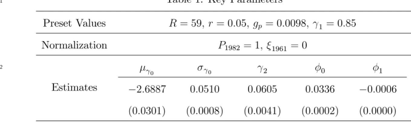
based on a priori information. The retirement age R and the interest rate r are 5910 and 4
0:05, respectively. The relative price of educational goods is assumed to increase over time 5
with a continuous growth rate denoted bygp. The growth rategpis set to0:0098by …tting an 6
exponential trend to the relative price of educational goods over the period of1908 to2004. 7
The price of educational goods in 1982is normalized to one. I also normalize the parameter 8
1961for utility from education of 1961 birth cohort to zero. Neither normalization a¤ects the 9
quantitative results in section 5. The curvature parameter 1 for human capital production 10
through schooling is not estimated here. The parameter 1 determines the curvature of 11
individual human capital pro…le across grades while in school. Without data on premarket 12
human capital stocks, it is hard to identify 1. The value of 1 is set to 0:85 following 13
Heckman et al. (1998).11 These values are summarized in the …rst two rows of Table 1.
14
Given these values, remaining parameters are estimated. I begin by introducing func-tional forms for the ability distribution and the human capital accumulation process after completion of schooling. Individual learning ability 0 is log-normally distributed with mean 0 and standard deviation 0. The process of human capital accumulation during the
postschooling period is given by
(a s) = 0(a s) + 1(a s)2 f or a s 9See the Online Appendix for more details on how to compute the skill prices. 10This corresponds to a real life age of65
:
11There is little literature that estimates the curvature parameter using data on premarket human capital
stocks, which is comparable to 1in this study. Heckman et al. (1998) consider a Ben-Porath-type lifetime human capital production technology and estimate the curvature 1 using wage data. Their estimates are 0.83 for high school graduates and 0.87 for college graduates. I use the average for my estimation.
With these functional forms, I have …ve parameters f
0; 0; 2; 0; 1g to estimate for the
1
human capital production function, where 2is the elasticity of human capital with respect to 2
expenditure. The estimation also involves 82 parametersf 1902; : : : ; 1960; 1962;: : : ; 1984gfor 3
cohort-speci…c utility from education. These 87 parameters are estimated by the generalized 4
method of moments (GMM) method, minimizing the weighted distance between a total of 88 5
data moments and their model counterparts. The moments include the following three sets: 6
i) the estimated return to schooling and quadratic return to experience from a pooled sample 7
Mincer regression (3 moments); ii) the mean years of schooling of 1902 through 1984 birth 8
cohorts12 and the variance of educational attainment of the 1961 birth cohort (84 moments);
9
and iii) the expenditure share of the net marginal cost of schooling (equation (3), 1 moment). 10
The …rst set of moments are Mincer coe¢ cients from the data and from the model. Using 11
a CPS pooled sample, I regress individual log hourly wages on years of schooling, potential 12
experience and its square, and year dummies along with other individual characteristics.13 13
The estimated coe¢ cients on years of schooling and potential experience and its square 14
from this Mincer regression are the …rst set of data moments. Their model counterparts are 15
computed from a model-based Mincer regression. Since education levels are discrete in the 16
data in contrast with the model, individuals in each cohort are collected in 18 education bins 17
(0to 17years of schooling) in the model, based on their proportions in the data. Given the 18
model parameters, the mean log human capital stock of every bin is computed. The model 19
moments in the …rst category are the corresponding coe¢ cients from a Mincer regression 20
with the sum of the mean log human capital stock and the log skill price as a dependent 21
variable.14
22
The second set of data moments are the mean years of schooling of 1902 through 1984 23
12See Figure 3.
13The control variables include gender, race, marital status, part-time status, census division of residence,
and standard metropolitan statistical area (SMSA) status.
14Running a Mincer regression based on the mean log human capital stocks yields the same coe¢ cients as
birth cohorts and the variance of educational attainment of the 1961 birth cohort in the CPS 1
sample. The corresponding model moments are computed by solving the model. 2
The last moment or the expenditure share in the net marginal cost of schooling is based on 3
equation (3). Unlike the …rst two sets of data moments, the expenditure share is constructed 4
for a given set of parameters. Since school expenditure is chosen by the median ability 5
person in each cohort, equation (3) holds only for the median ability person. I …rst solve 6
the optimal educational attainment of the median ability person (with learning abilitye 0)
7
in each cohort. Given this level of education, the time path of skill prices and cohort-level 8
educational expenditures15 are used to compute the expenditure share of the net marginal
9
cost of schooling for each cohort. The mean expenditure share over all cohorts is the third 10
set of data moment. As equation (3) indicates, its model counterpart is the expenditure 11
elasticity 2 of human capital. 12
Having constructed the data and the model moments this way, I estimate the parame-ters using the GMM. In implementing the estimation, the parameparame-ters are divided into two groups: i) 1 = f 0; 0; 2; 0; 1g for the human capital production function; and ii) 2 = f 1902; : : : ; 1960; 1962;: : : ; 1984g for cohort-speci…c utility from education. First, …nd 2 that exactly replicates the relevant cohort mean years of schooling (82moments), for any
given 1. Then, minimize the weighted distance between the remaining six data moments16
and their model counterparts over 1. The parameter estimates b1 for the human capital
production function can be written as
b1 = arg min 1g( 1)0W g( 1);
where g( 1) =md m( 1); md is the vector of data moments, m( 1)is the vector of model 13
15See the Online Appendix for more details on how to compute cohort-level educational expenditure. 16The moments include the Mincer coe¢ cients on years of schooling, potential experience and its square,
the mean and the variance of educational attainment of the 1961 birth cohort, and the expenditure share of the net marginal cost of schooling.
moments evaluated at a given set 1 of parameters, and W is the weighting matrix. Re-1
gardless of the choice of the weighting matrixW, the estimator is consistent. The weighting 2
matrix used for the estimation is the inverse of a diagonal matrix, whose elements are the 3
variances of the data moments. Since the last data moment (or the expenditure share of the 4
net marginal cost of schooling) depends on the model parameters, its variance is computed 5
based on the parameter estimates from a model without utility from education. Standard 6
errors for the estimates are calculated based on numerical di¤erentiation. 7
5. Results
8
This section starts with a discussion of the estimates for the human capital production 9
function. It then presents the main growth accounting results, followed by a sensitivity 10
analysis. 11
5.1. Parameter Estimates and the Fit of the Model
12
Parameter estimates for the distribution of learning ability and the human capital pro-13
duction function are reported in the last row of Table 1. The baseline model estimates the 14
expenditure elasticity 2 of human capital, which is key to understanding the impact of rising 15
school spending on labor quality growth, to be 0:06. This implies that school expenditures 16
explain about6%of the net marginal cost of schooling as represented by equation (3). Para-17
meter estimates for 0 and 1con…rm that the postschooling evolution of human capital with 18
work experience is steeper than the cross-sectional experience-earnings pro…les due to the 19
rise in school quality. According to the estimates, individual human capital increases by63% 20
with 30 years of work experience and the cross-sectional return to experience understates 21
this actual return by more than 7%. 22
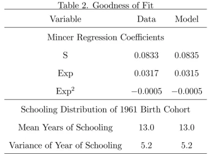
The model matches empirical Mincer coe¢ cients well as shown in Table 2. Both return 23
to schooling and quadratic return to experience from the model-based Mincer regression are 24
very close to those in the data. The model is also consistent with the rise in the estimated 1
Mincer returns to schooling over time in the CPS data. Figure 4 plots the trends in the 2
Mincer return to schooling from the baseline model together with those in the data. Even if 3
the Mincer return to schooling from the pooled sample is targeted, the model is well in line 4
with the rise in the year-by-year Mincerian returns to schooling in the CPS data over the 5
period 1967 to 2000.17 6
Can we let the rise in school quality take all the credit for this rapid increase in the 7
estimated returns to schooling? A vast literature on wage inequality in the U.S. for the past 8
few decades18 suggests that the increases in relative wages of more educated workers for the
9
period is largely due to a rising demand for them. In order to quantify how much of the rise 10
in the estimated return to schooling in the data is attributable to the growth in school quality 11
and a rising skill premium, respectively, a counterfactual exercise is implemented. The gray 12
solid line in Figure 4 represents the time path of Mincer return to schooling implied by the 13
model, assuming that the skill premium stayed constant for the sample period at its 1967 14
level. Without the rise in the skill premium, the Mincerian return to schooling increases 15
by less than 1 percentage point between 1967 and 2000, which explains only 12% of the 16
total increase in the Mincer return to schooling in the baseline model. This con…rms that 17
a signi…cant part of the rise in the estimated returns to schooling results from an increased 18
skill premium, not from better quality of schooling for more recent cohorts. 19
The model can replicate the mean and the variance of educational attainment of the 1961 20
birth cohort as Table 2 presents. By introducing cohort-speci…c parameters for utility from 21
schooling, the model exactly matches the time series of the cohort mean years of schooling. 22
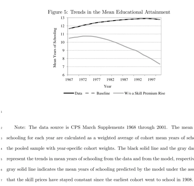
This enables the model to generate the evolution of mean educational attainment in the 23
17The model slightly overstates the increase in the Mincer returns to schooling, which is attributable to
the fact that I use skill prices for four education windows instead of 18 discrete levels of schooling. However, this is inevitable because the numbers of observations in some education groups are small.
18Figure 2 presents the trends in wage gap between college graduates and high school graduates in the
CPS data between 1967 and 2000 as shown in Figure 5.19 How important is the rise in
1
skill premium in explaining the increases in mean years of schooling of the U.S. workforce? 2
The gray solid line in Figure 5 plots the time path of mean years of schooling predicted by 3
the model, assuming that all skill prices grew at the same rate without a rise in the skill 4
premium. The mean level of educational attainment of the workforce increases initially as 5
the average wages rise. However, it turns to a declining trend since the mid-1970s because 6
the relative price of educational goods grows more rapidly than the average wages. Without 7
the rise in the skill premium, the model cannot generate a secular rise in the mean years of 8
schooling in the data. 9
5.2. Growth Accounting
10
This subsection discusses the main quantitative results based on the estimated parame-11
ters. Following the growth accounting framework proposed in section 2, two components 12
of labor quality growth (labor composition growth (Hc) and human capital quality growth 13
(Hq)) are computed for any two consecutive years. 14
Table 3 presents my growth accounting results with those from the BLS’s approach. The 15
growth rates of labor productivity and physical capital inputs in all panels are taken from 16
the BLS. The TFP growth is obtained as a residual after accounting for growth in physical 17
capital and labor quality. The contributions of both physical capital growth and labor quality 18
growth presented in Table 3 are adjusted for their cost shares. 19
As the second panel in Table 3 shows, human capital of the U.S. workforce increased by 20
0:4% per year between 1967 and 2000, with 20% of this explained by the growth in school 21
quality.20 This implies that rising educational spending is about one-fourth as important
22
19The mean years of schooling for each year are calculated as a weighted average of cohort mean years of
schooling in the pooled sample with year-speci…c cohort weights.
20The BLS labor composition growth is smaller than my estimate. This is because my growth accounting
framework views workers with di¤erent education and potential experience as di¤erent labor inputs, while the BLS additionally considers gender in classifying workers. Since women on average earn less than men, increased female labor force participation in the past decades lowers the BLS measure of labor composition
as increases in mean years of schooling for U.S. labor productivity growth for the period.21
1
Given the drastic rise in real school expenditures per pupil during the 20th century, U.S. 2
labor quality growth has been fairly modest. The total labor quality growth due to rises 3
in both the quantity and quality of schooling explains about one-quarter of the U.S. labor 4
productivity growth between1967and2000. With this new measure of labor quality growth, 5
the TFP growth rate declines. I …nd that the contribution of growth in TFP to U.S. labor 6
productivity growth is about a quarter, compared with the 40% reported by the BLS. 7
5.3. Sensitivity Analysis 8
A couple of subsamples are considered for sensitivity analysis. First, the model para-9
meters are reestimated with data on males to remove any e¤ect of signi…cant changes in 10
women’s selection into the labor force in recent decades on the estimate. The estimation is 11
also repeated using a sample of FTFY workers since the model rules out part-time workers 12
included in the baseline estimation. Since data on educational expenditures are not available 13
separately for these subsamples, the same data on educational expenditures are used for both 14
exercises. The growth accounting results with these two subsamples are summarized in the 15
bottom two panels of Table 3. 16
Using the male sample, the estimated labor composition growth is reduced to0:29% from 17
0:32% in the baseline model. Recall that labor composition growth is mainly determined 18
by increases in educational attainment. The smaller estimate for labor composition growth 19
among men implies that the female workforce composition has changed toward more educated 20
and more experienced workers relative to the male workforce. 21
However, this did not accompany better quality of schooling for women relative to men. 22
Human capital quality growth among men is 0:10%, larger than the baseline estimate. One 23
growth relative to my estimate.
21Labor composition growth also includes the impact of changes in the experience composition of the
workforce on labor quality growth. Since the mean years of experience of the U.S. workforce do not show any secular trend, their quantitative impact on labor composition growth is small.
explanation is related to changing selection in schooling choice. Given a cohort-invariant dis-1
tribution of learning ability, increases in mean years of schooling are associated with a lower 2
mean ability for any given years of schooling among recent cohorts. Thus, a greater increase 3
in the mean educational attainment among women lowers human capital quality growth in 4
the baseline model, relative to that with the male sample. In addition, a narrowing gen-5
der gap may a¤ect the estimated human capital quality growth. As the gender gap declines, 6
women have greater incentives to spend more while in school because they anticipate a higher 7
rate of return to educational expenditure than men. Given this incentive, expenditures are 8
estimated to be less e¤ective in increasing human capital among women than among men 9
because the same school expenditures are assumed for both men and women. 10
The last panel of Table 3 shows that the estimated labor quality growth among FTFY 11
workers is little di¤erent from that in the baseline model. Both labor composition growth 12
and human capital quality growth are 0:01percentage point lower with FTFY workers than 13
with the whole sample. The baseline quantitative results are robust to excluding part-time, 14
part-year workers from the sample. 15
6. Conclusion
16
Building upon Denison (1962), the BLS incorporates labor quality growth as a source of 17
U.S. labor productivity growth. Although the BLS measure of labor quality growth adjusts 18
for the increases in mean years of schooling of the workforce, it fails to capture any impact of 19
the rise in school quality. Public school spending per pupil in the U.S. increased drastically 20
during the 20th century. If this contributed to the quality of U.S. education, then the BLS 21
approach underestimates labor quality growth. 22
This paper measures how much U.S. labor quality has risen in response to the increase in 23
public school expenditures per pupil. To this aim, it is critical to identify the productivity 24
of educational spending in human capital production. This paper proposes a new way 25
of estimating this productivity by exploiting a schooling model as well as cross-sectional 1
earnings di¤erences across cohorts. 2
The main …nding is that U.S. labor quality increased by0:4% per year between1967 and 3
2000, one-…fth of which is attributable to the rise in school expenditure. This implies that 4
about a quarter of U.S. labor productivity growth can be accounted for by labor quality 5
growth for the same period. The estimated impact of the increased educational spending on 6
growth in U.S. labor quality is greater among men, whereas the baseline result is similar to 7
that with FTFY workers. I also …nd that the growth in school quality explains only 10% of 8
the rise in empirical Mincer return to schooling for the sample period, while the remainder 9
is due to a rising skill premium. 10
This study abstracts from the causes of the increase in school expenditures and focuses 11
on its impact on labor quality growth. The modest impact of the increased educational 12
expenditure on the growth in human capital estimated in this paper raises a question of 13
what has driven such a drastic rise in spending on schooling. Exploring this may help us 14
better understand the role of education in U.S. economic growth. 15
References
1
Ben-Porath, Y., 1967. The production of human capital and the life cycle of earnings. Journal 2
of Political Economy 75 (4), 352–365. 3
Betts, J. R., 1995. Does school quality matter? evidence from the national longitudinal 4
survey of youth. Review of Economics and Statistics 77 (2), 231–250. 5
Bils, M., Klenow, P. J., 2000. Does schooling cause growth? American Economic Review 6
90 (5), 1160–1183. 7
Dearden, L., Ferri, J., Meghir, C., 2002. The e¤ect of school quality on educational attain-8
ment and wages. Review of Economics and Statistics 84 (1), 1–20. 9
Denison, E. F., 1962. The Sources of Economic Growth in the United States and the Alter-10
natives Before Us. Committee for Economic Development, New York. 11
Erosa, A., Koreshkova, T., Restuccia, D., 2010. How important is human capital? a quanti-12
tative theory assessment of world income inequality. Review of Economic Studies 77 (4), 13
1421–1449. 14
Hall, R. E., Jones, C. I., 1999. Why do some countries produce so much more output per 15
worker than others? Quarterly Journal of Economics 114 (1), 83–116. 16
Hanushek, E. A., 1986. The economics of schooling: Production and e¢ ciency in public 17
schools. Journal of Economic Literature 24 (3), 1141–1177. 18
Hanushek, E. A., Rivkin, S. G., 1997. Understanding the twentieth-century growth in u.s. 19
school spending. Journal of Human Resources 32 (1), 35–68. 20
Hanushek, E. A., Rivkin, S. G., Taylor, L. L., 1996. Aggregation and the estimated e¤ects 21
of school resources. Review of Economics and Statistics 78 (4), 611–627. 22
Heckman, J. J., Layne-Farrar, A. S., Todd, P. E., 1996. Human capital pricing equations 1
with an application to estimating the e¤ect of schooling quality on earnings. Review of 2
Economics and Statistics 78 (4), 562–610. 3
Heckman, J. J., Lochner, L., Taber, C., 1998. Explaining rising wage inequality: Expla-4
nations with a dynamic general equilibrium model of labor earnings with heterogeneous 5
agents. Review of Economic Dynamics 1 (1), 1–58. 6
Klenow, P. J., Rodríguez-Clare, A., 1997. The neoclassical revival in growth economics: Has 7
it gone too far? NBER Macroeconomics Annual, 73–114. 8
Manuelli, R. E., Seshadri, A., 2007. Human Capital and the Wealth of Nations. Mimeo. 9
National Center for Education Statistics, 1993. 120 Years of American Education: A Statis-10
tical Portrait. U.S. Department of Education, Washington D.C. 11
National Center for Education Statistics, 2004. Digest of Education Statistics. U.S. Depart-12
ment of Education, Washington D.C. 13
Rangazas, P., 2002. The quantity and quality of schooling and u.s. labor productivity growth 14
(1870-2000). Review of Economic Dynamics 5 (4), 932–964. 15
Warren, G. F., Pearson, F. A., 1935. Gold and Prices. John Wiley and Sons, New York. 16
Table 1. Key Parameters 1 Preset Values R = 59; r= 0:05; gp = 0:0098; 1 = 0:85 Normalization P1982 = 1; 1961 = 0 Estimates 0 0 2 0 1 2:6887 (0:0301) 0:0510 (0:0008) 0:0605 (0:0041) 0:0336 (0:0002) 0:0006 (0:0000) 2
Note: Numbers in parentheses stand for standard errors.
Table 2. Goodness of Fit 1
Variable Data Model
Mincer Regression Coe¢ cients
S 0:0833 0:0835
Exp 0:0317 0:0315
Exp2 0:0005 0:0005
Schooling Distribution of 1961 Birth Cohort Mean Years of Schooling 13:0 13:0
Variance of Year of Schooling 5:2 5:2 2
Note: The data source is CPS March Supplements 1968 through 2001. Mincer coe¢ cients
3
from the data are based on a pooled-sample regression of individual log hourly wages on years
4
of schooling, potential experience and its square, gender, race, marital status, part-time status,
5
census division of residence, SMSA status, and year dummies. The mean and the variance of years
6
of schooling are based on the data of 1961 birth cohorts in the pooled sample of 1968 through 2001
7
surveys.
Table 3. Decomposition of Labor Productivity Growth Between 1967 and 2000 1
Y =L T F P K=L H (Labor Quality)
Hc (Labor Composition) Hq (Human Capital Quality) BLS (Private Business Sector)
1:66 0:67 0:77 0:22 :: Baseline Model 1:66 0:49 0:77 0:32 (0:00) 0:08 (0:01) Men only 1:66 0:50 0:77 0:29 (0:00) 0:10 (0:01) FTFY only 1:66 0:51 0:77 0:31 (0:00) 0:07 (0:01) 2
Note: The unit is percent. Numbers in parentheses stand for standard errors. Growth rates of
3
labor productivity (Y =L) and capital-labor ratio (K=L) are from the BLS multifactor productivity
4
tables. Growth rates of total factor productivity (T F P) are obtained as residuals.
5
Figure 1: U.S. Real Expenditures Per Pupil in Public Elementary and Secondary Schools 2000 3000 4000 1982 $ 0 1000 1908 1918 1928 1938 1948 1958 1968 1978 1988 1998 Year
Note: Data sources include the National Center for Education Statistics (1993) and the National
1
Center for Education Statistics (2004). The time series is the yearly total expenditure per pupil
2
in public elementary and secondary schools. For the period during which the data were collected
3
biennially, a cubic spline is used to interpolate the series. The series is de‡ated by the price index
4
for PCE on education services where the data permit. Since the de‡ator is not available before
5
1929, I use the projection of the price index for PCE on education on the CPI by splicing it to
6
actual data since 1929. For the years before 1913, during which the CPI was unavailable, the price
7
index in Warren and Pearson (1935) is used.
Figure 2: Trends in Wage Gap Between College Graduates and High School Graduates in the U.S. 0.4 0.5 0.6 o g W age D iffe re nt ia l 0.2 0.3 1967 1977 1987 1997 Year L o 1
Note: The data source is CPS March Supplements 1968 through 2001. Since wages in the
2
survey data are for the previous calendar year, the …gure covers the period 1967 through 2000 even
3
if the survey years are 1968 through 2001. Wage gap is de…ned as the mean log wage di¤erential.
4
College graduates are those with 16 years of schooling or a college degree, and high school graduates
5
are those with 12 years of schooling or a high school diploma.
Figure 3: The Mean Years of Schooling Across Cohorts 11 12 13 14 15 n Ye ar s of Sc h o o lin g 8 9 10 1902 1912 1922 1932 1942 1952 1962 Birth cohort Mea n 1
Note: The data source is CPS March Supplements 1968 to 2001. The pooled sample of 1968 to
2
2001 surveys is used to compute the mean years of schooling of each cohort.
Figure 4: Trends in the Estimated Mincerian Returns to Schooling: Data vs. Model 0.08 0.10 0.12 0.14 Rate of R eturn 0.04 0.06 1967 1972 1977 1982 1987 1992 1997
Data Baseline W/o a Skill Premium Rise Year
1
Note: The data source is CPS March Supplements 1968 through 2001. Since wages in the
2
survey data are for the previous calendar year, the …gure covers the period 1967 through 2000
3
even if the survey years are 1968 through 2001. The black solid line represents the trends in the
4
estimated coe¢ cient on years of schooling from year-by-year Mincer regressions of individual log
5
hourly wages on years of schooling, potential experience and its square, gender, race, marital status,
6
part-time status, census division of residence, and SMSA status. The gray dashed line indicates
7
the time series of the estimated return to schooling from a model-based Mincer regression for each
8
year. The gray solid line represents a counterfactual trend in the Mincerian return to schooling
9
assuming that the skill prices stay constant at their 1967 levels.
Figure 5: Trends in the Mean Educational Attainment 8 9 10 11 12 13 ean Y ears of Sch ooli n g 6 7 1967 1972 1977 1982 1987 1992 1997
Data Baseline W/o a Skill Premium Rise Year
M
e
1
Note: The data source is CPS March Supplements 1968 through 2001. The mean years of
2
schooling for each year are calculated as a weighted average of cohort mean years of schooling in
3
the pooled sample with year-speci…c cohort weights. The black solid line and the gray dashed line
4
represent the trends in mean years of schooling from the data and from the model, respectively. The
5
gray solid line indicates the mean years of schooling predicted by the model under the assumption
6
that the skill prices have stayed constant since the earliest cohort went to school in 1908.