A
University
of
Sussex
DPhil
thesis
Available
online
via
Sussex
Research
Online:
http://sro.sussex.ac.uk/
This
thesis
is
protected
by
copyright
which
belongs
to
the
author.
This
thesis
cannot
be
reproduced
or
quoted
extensively
from
without
first
obtaining
permission
in
writing
from
the
Author
The
content
must
not
be
changed
in
any
way
or
sold
commercially
in
any
format
or
medium
without
the
formal
permission
of
the
Author
When
referring
to
this
work,
full
bibliographic
details
including
the
author,
title,
awarding
institution
and
date
of
the
thesis
must
be
given
Large-Scale Photometric Surveys
Leon Baruah
Submitted for the degree of Doctor of Philosophy University of Sussex
Declaration
I hereby declare that this thesis has not been and will not be submitted in whole or in part to another University for the award of any other degree.
Signature:
UNIVERSITY OF SUSSEX
Leon Baruah, Doctor of Philosophy
A Galaxy Cluster Finding Algorithm for Large-Scale Photometric Surveys
Summary
As the largest gravitationally bound objects in the Universe, galaxy clusters can be used to probe a variety of topics in astrophysics and cosmology. This thesis describes the development of an algorithm to find galaxy clusters using non-parameteric methods applied to catalogs of galaxies generated from multi-colour CCD observations. It is motivated by the emergence of increasingly large, photometric galaxy surveys and the measurement of key cosmological parameters through the evolution of the cluster mass function.
The algorithm presented herein is a reconstruction of the successful, spectroscopic cluster finding algorithm, C4 (Miller et al., 2005), and adapting it to large photometric
surveys with the goal of applying it to data from the Dark Energy Survey (DES).AperC4
uses statistical techniques to identify collections of galaxies that are unusually clustered in a multi-dimensional space. To characterize the new algorithm, it is tested with simulations produced by the DES Collaboration and I evaluate its application to photometric datasets.
In doing so, I show howAperC4 functions as a cosmology independent cluster finder and
formulate metrics for a “successful” cluster finder.
Finally, I produce a galaxy catalog appropriate for statistical analysis. C4 is applied to the SDSS galaxy catalog and the resulting cluster catalog is presented with some initial analyses.
“There is a single light of science, and to brighten it anywhere is to brighten it everywhere.”
Acknowledgements
I am grateful to Dr Kathy Romer, Prof. Chris Miller, and Dr Jon Loveday, who took on various supervisory roles during the course of this Ph.D. I cannot undervalue the thanks I owe my main supervisor, Kathy Romer, for taking me on as a student, for her thorough proof-reading of this thesis, and lending her support when I really needed it. I am indebted to the help of Chris Miller, who provided me with the original C4 algorithm that formed the basis of this thesis. I would like to thank him for his constructive advice, for hosting me at Michigan, for the time he has spent helping me flesh out my ideas and putting me on the right track when I was in need of direction. His generous donation of compute time on the FLUX HPC cluster made this thesis possible.
I am also grateful to the Astronomy department at Sussex for their advice over the years: I heard it well even though some of it may have taken time to sink in! Further thanks go to Andrew Liddle whose willingness to sit and listen to me and kind advice will not be forgotten.
Thank you to my examiners, Jon Loveday and Alfonso Arag´on-Salamanca, for their
considered feedback and hugely thoughtful input to the full development of this thesis. Numerical computations were done on the Sciama High Performance Compute (HPC) cluster (supported by the ICG, SEPNet and the University of Portsmouth), and the FLUX HPC cluster at the University of Michigan (UMich). I would like to acknowledge financial support from 2007 to 2011 through a Science and Technology Facilities Council student-ship. I was also able to attend various DES collaboration meetings thanks to funding from STFC, Ohio State University, and the DES collaboration itself. I attended an NVO Summer School part funded by NVO and received funding for my visit to Michigan.
This thesis would also not have been possible if it weren’t for key contributions from around the world. I’d like to thank the many faces of the DES collaboration, who have been both welcoming and inspiring in many ways during my studentship. I must thank the DES simulations team, particularly Michael Busha and Risa Wechsler for driving the production and high quality of the DES Catalog Simulations. I thank Brian Gerke for sharing his membership matching code, and allowing me to collaborate in its development. I am
grateful for Dongryeol Lee’s technical assistance and advice on thekth Nearest Neighbour finder. I must thank Gary Burton for technical assistance and his prompt, helpful, and friendly support, on using the Sciama computing cluster at Portsmouth. I also thank Peter Thomas for donating IDL licenses to the Sciama cluster, which in turn permitted me to use it.
I’d like to thank the many people who I’ve lived with during my Ph.D., and tolerated my sometimes-possibly-coherent rambles, here (in no particular order): Lauren Coleman, Matt Ryan, Sophie Osborne, Isaac & Yuko Roseboom, Cath Berry, Alex Seabrook, Tabitha
Rohrer, Ness Kabas, Bernard Mills, and Monica Ross. They have made my time in
Brighton all the richer in many ways. I’m particularly thankful to Pete Offord, Antony Lewis, and Ruth Pearson, for giving me a place to stay during my hauntingly regular spates of homelessness.
I must thank my fellow starting DPhil students, whose respective journeys have been inspirational; particularly Anna Jordanous and Sandra Deshors, whose continued friend-ship and support have been a lifeline.
Likewise, I would like like to thank my many friends and coworkers at the Physics and Astronomy dept, those that have since left, as well as those that since come and gone, for their help (and hindrance!) over the years, and making Sussex an enjoyable place to be. Special shout outs go to (in no particular order): David Parkinson, Leonidas Christodoulou, Duncan Farrah, Will Demeri-Watson, Donough Regan, Gemma Anderson, Darren Baskill, Nicola Mehrtens, Matt Thomson, Ippocratis Saltas, and Gwen Lefeuvre; all of whom have given me respite from sanity and insanity alike, and have broadened my horizons.
Finally, I thank my family, Richie, Manju, and Dwijen, for their continued love and support and for always just being there. Their belief in me from the time that I started this journey up until the present day has been unwavering; I don’t know where I would be without it. This is for you.
Contents
List of Tables xii
List of Figures xv
1 Introduction 1
1.1 Introduction to Cosmology . . . 1
1.1.1 The Cosmic Expansion . . . 1
1.1.2 Dark Energy . . . 4
1.2 Introduction to Galaxy Clusters . . . 4
1.2.1 History . . . 4
1.2.2 Galaxy Clusters as Astrophysical Probes . . . 6
1.3 Cosmological Constraints from Galaxy Clusters . . . 9
1.3.1 Cosmological Measurements with Cluster Counts . . . 10
1.4 Observations of Galaxy Clusters . . . 11
1.4.1 Optical . . . 12
1.4.2 X-ray . . . 14
1.4.3 Microwave . . . 14
1.5 Optical Cluster Finding . . . 15
1.5.1 History of optical cluster finding . . . 15
1.5.2 Red Sequence . . . 16
1.5.3 MaxBCG . . . 16
1.5.4 Voronoi Tesselation . . . 17
1.5.5 Cut and Enhance . . . 18
1.5.6 C4 . . . 18
1.6 Evaluating Cluster Finders . . . 19
2 The Original C4 Algorithm 22
2.1 SDSS DR2 . . . 22
2.1.1 The Sloan Digital Sky Survey (SDSS) . . . 22
2.1.2 Selection of Spectroscopic DR2 Galaxy Catalog . . . 26
2.2 The Original C4 Cluster Finding Algorithm . . . 29
2.2.1 Introductory Notes . . . 30
2.2.2 C4-clustering . . . 31
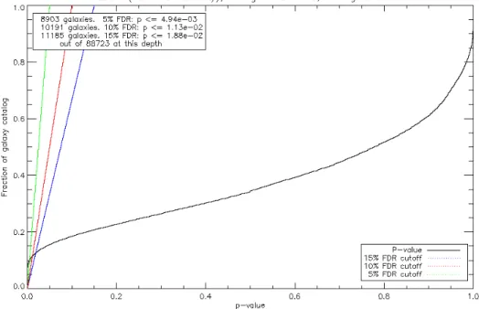
2.2.3 False Discovery Rate (FDR) . . . 35
2.2.4 k-NN Distance . . . 39
2.2.5 Assigning Galaxies to Clusters . . . 40
2.3 Results of the Miller et al. Application of C4 to SDSS DR2 . . . 41
2.3.1 Purity and Completeness . . . 41
2.3.2 Calibrating C4 Parameters . . . 42
2.3.3 Fiber Collisions . . . 43
2.3.4 Comparison to Other Cluster Catalogs . . . 44
2.3.5 Follow-on Work . . . 45
2.4 Shortcomings of C4 . . . 46
2.4.1 Spectroscopic Redshift Limitations . . . 46
2.4.2 Association of Galaxies to Clusters . . . 46
2.4.3 Cosmology . . . 47
2.4.4 Ease of Use . . . 47
2.5 Summary . . . 48
3 AperC4: a New Cluster Finding Algorithm 49 3.1 Motivations for Modifications . . . 49
3.1.1 Why Modify C4? . . . 49
3.1.2 Redshift Considerations . . . 50
3.1.3 On Apertures and Cosmology . . . 51
3.1.4 Computational Modifications . . . 51
3.2 Introduction to the New Algorithm . . . 53
3.2.1 AperC4 Algorithm Outline . . . 53
3.2.2 Step 1. Survey treatment: Tiling . . . 54
3.2.3 Step 2. AperC4-clustering: p-value Measurement . . . 55
3.2.4 Step 3. Identify C4 galaxies . . . 58
3.2.6 Step 5. Forming Clusters . . . 59
3.2.7 Step 6. Assignment of Redshift to Clusters . . . 60
3.2.8 Step 7. Accounting for Fragmented Clusters . . . 62
3.2.9 Step 8. Richness Cut . . . 63
3.2.10 AperC4 Algorithm Input Parameters . . . 63
3.3 Discussion . . . 67
3.3.1 p-value Calculation with Defined Apertures . . . 67
3.3.2 Aperture Gedanken . . . 68
3.3.3 p(z) Blending and Fragmentation . . . 73
3.3.4 Comparison of AperC4 and C4M05 Algorithms . . . 75
3.4 Summary . . . 80
4 Introduction to DES and CatSim 82 4.1 The Dark Energy Survey (DES) . . . 82
4.1.1 Overview . . . 82
4.1.2 DECam . . . 83
4.2 Cosmology with DES . . . 84
4.2.1 Weak Lensing . . . 84
4.2.2 Galaxy Clustering . . . 85
4.2.3 Type Ia Supernovae . . . 85
4.2.4 Clusters of Galaxies . . . 86
4.3 DES Catalog Simulations . . . 87
4.3.1 Introduction to CatSim . . . 87
4.3.2 Simulation Construction . . . 87
4.3.3 CatSim Products . . . 89
4.4 Summary . . . 91
5 Evaluating Cluster Finding 92 5.1 Evaluation Measures . . . 92
5.1.1 Completeness and Purity . . . 92
5.1.2 Unique Matching . . . 94
5.1.3 F-measure . . . 94
5.2 Method of Evaluation . . . 95
5.2.1 Membership Matching . . . 95
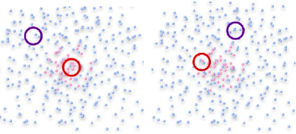
5.2.3 Gerke Matching Algorithm . . . 97
5.2.4 Modified Matching Algorithm . . . 101
5.2.5 Redshift Binning . . . 102
5.2.6 Matching Algorithm Output . . . 103
5.3 Ranking the AperC4 Clusters by Mass Proxy . . . 111
5.3.1 Ngals Ranking . . . 111
5.3.2 Abell Ranking . . . 112
5.4 Testing the Matching Code . . . 113
5.4.1 Pure and Complete Cluster Catalog . . . 113
5.4.2 Impure and Complete Cluster Catalog . . . 113
5.4.3 Incomplete and Pure Cluster Catalog . . . 113
5.4.4 Incomplete and Impure Cluster Catalog . . . 116
5.4.5 Ranking byNgals . . . 116
5.4.6 Ngals Limited Catalogs . . . 116
5.5 Summary . . . 119
6 Characterisation of AperC4 with SDSS Catalog Simulations 120 6.1 CatSim Implementation of zCarlosp(z) . . . 120
6.1.1 Introduction to zCarlosp(z) Method . . . 120
6.1.2 zCarlos Applied to CatSim . . . 122
6.1.3 zCarlosp(z) of CatSim Halos . . . 123
6.2 AperC4 Applied to CatSim . . . 125
6.3 Optimal Parameter Selection with p(z) Information . . . 127
6.3.1 Optimisation using zCarlos . . . 127
6.3.2 Idealisedp(z) Information . . . 129
6.3.3 Optimal Parameter Set . . . 129
6.4 Discussion . . . 132
6.4.1 AperC4 Catalog Statistics with zCarlos Redshifts . . . 132
6.4.2 AperC4 Catalog Statistics with Ideal Redshifts . . . 137
6.4.3 Comparison between zCarlos and Ideal Redshift Cluster Catalogs . . 140
6.5 Summary . . . 142
7 The SDSS DR8-AperC4 catalog 144 7.1 SDSS DR8 . . . 144
7.1.2 Sheldon et al. Galaxy Selection . . . 146
7.1.3 Galaxy Selection for AperC4 . . . 147
7.1.4 Magnitude Limits . . . 151
7.2 AperC4-SDSS DR8 Cluster Catalog Assembly . . . 153
7.2.1 Survey Tiling . . . 153
7.2.2 p-value Determination and FDR . . . 153
7.2.3 k-NN Centre Determination and Forming Aperture-Slice Clusters . . 156
7.2.4 Combining the Aperture-Slice Clusters with p(z) Information and Producing the Final Cluster Catalog . . . 158
7.3 The AperC4-SDSS DR8 Cluster Catalog . . . 159
7.3.1 AperC4-SDSS DR8 Catalog Summary . . . 159
7.3.2 GAMA Spectroscopy in AperC4-SDSS DR8 Clusters . . . 163
7.3.3 Example AperC4 Clusters with GAMA Redshifts . . . 165
7.4 Discussion . . . 168
7.4.1 AperC4-SDSS DR8 Structure . . . 168
7.4.2 Potential Improvements to AperC4 . . . 173
7.5 Summary . . . 175
8 Thesis Summary and Further Work 176 8.1 Summary of Thesis . . . 176
8.2 Further Work . . . 178
8.2.1 Algorithm Development . . . 178
8.2.2 Evaluation Framework . . . 179
8.2.3 Uses for the AperC4-SDSS DR8 catalog . . . 180
List of Tables
2.1 Transformation between R.A./dec and SDSS survey coordinates . . . 23
3.1 Parameters of the AperC4 algorithm . . . 64
3.2 Parameters that augment the AperC4 algorithm . . . 66
3.3 Physical Scales of Aperture Radii assuming a WMAP-9 Cosmology . . . 69
6.1 Variables tested on CatSim with the AperC4 algorithm . . . 126
6.2 Optimal AperC4 parameter sets for CatSim DR8 catalog with zCarlos red-shifts . . . 129
6.3 Optimal AperC4 parameter sets for CatSim DR8 catalog with simulation redshifts . . . 131
7.1 AperC4 cluster catalog schema . . . 159
7.2 AperC4 member catalog schema . . . 159
List of Figures
1.1 Composite Optical, X-ray and Lensing map of galaxy cluster 1E 0657-56,
the “Bullet Cluster” . . . 8
1.2 Average spectrum of a Luminous Red Galaxy . . . 12
1.3 Example of a cluster with an identified BCG and red sequence . . . 13
2.1 SDSS filter transmission curves . . . 24
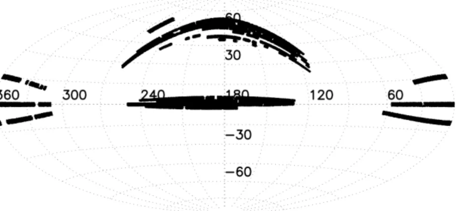
2.2 Aitoff projection of the coverage of SDSS DR2 spectroscopic campaign . . . 27
2.3 Evaluation of galaxies’ probabilities of lying in a colour box . . . 34
2.4 Comparison of a cluster galaxy and field galaxy in colour-colour space . . . 36
2.5 Types of errors that occur in hypothesis testing . . . 37
2.6 The trade-off between false discoveries and power . . . 38
3.1 Flowchart of the p-value evaluation process . . . 55
3.2 Distribution of p-values in DR2 . . . 58
3.3 Flowchart of the AperC4 process for a single aperture . . . 61
3.4 Key for gedanken figures . . . 69
3.5 Over-sized aperture gedanken . . . 70
3.6 Cluster-sized aperture gedanken . . . 71
3.7 Smaller cluster-sized aperture gedanken . . . 71
3.8 Undersized aperture gedanken . . . 72
3.9 Combining multiple aperture catalogs gedanken . . . 73
3.10 Redshifts of combined aperture catalog gedanken . . . 75
5.1 Key for ranking examples . . . 99
5.2 Incomplete catalog treatment by Gerke matching algorithm . . . 99
5.3 Impure catalog treatment by Gerke matching algorithm . . . 100
5.5 Example of a set of mass scatter plots produced by matching a CatSim AperC4 catalog non-uniquely . . . 105
5.6 Example of a set of mass scatter plots produced by matching a CatSim
AperC4 catalog uniquely . . . 106
5.7 Example of a set of purity and completeness plots for a CatSim AperC4
catalog . . . 108 5.8 Example of a set of centering plots for a cluster catalog . . . 110
5.9 Purity and completeness plots for a 50% impure CatSim catalog . . . 114
5.10 Purity and completeness plots for a 50% incomplete CatSim catalog . . . . 115 5.11 Mass scatter plots for anNgals ranked CatSim catalog . . . 117
5.12 Purity and completeness plots for a CatSim catalog limited to clusters where Ngals ≥32 . . . 118
6.1 N(z) of the CatSim DR8 galaxies . . . 123 6.2 Example zCarlos p(z)s of two CatSim halos . . . 124
6.3 Maximum F1 score by AperC4 parameter for zCarlos redshift information . 128
6.4 Maximum F1 score by AperC4 parameter for simulation redshift . . . 130
6.5 Non-unique scatter of matched AperC4-CatSim cluster-halos from the
op-timal AperC4 catalog. . . 133
6.6 Unique scatter of matched AperC4-CatSim cluster-halos from the optimal
AperC4 catalog . . . 134
6.7 Purity, Completeness, and F1 measure of matched AperC4-CatSim
cluster-halos from the optimal AperC4 catalog . . . 136
6.8 Purity, Completeness, and F1 measure of matched AperC4-CatSim
cluster-halos using simulation redshift . . . 138
6.9 Centering of matched AperC4-CatSim cluster-halos from the optimal AperC4
catalog . . . 139 6.10 Centering of matched AperC4-CatSim cluster-halos using simulation redshift141
7.1 Surface Brightness distribution of the Sheldon et al. DR8 Galaxy Sample . 149
7.2 Example ‘galaxies’ identified by surface brightness cut . . . 150
7.3 Magnitude histograms and limits determined from Sheldon et al. galaxy
catalog . . . 152 7.4 Distribution of DR8 galaxies and tiling of the BOSS footprint . . . 154 7.5 p-values of DR8 galaxies found with the 3.70 aperture . . . 155
7.6 Aperture-slice cluster distributions from 3 apertures . . . 157
7.7 Distribution of AperC4-DR8 clusters across the BOSS survey footprint. . . 161
7.8 N(z) of AperC4-DR8 clusters. . . 162
7.9 Ngals of AperC4-DR8 clusters. . . 162
7.10 Mean GAMA galaxy redshifts against peak AperC4 clusterp(z) . . . 164
7.11 Dispersion of AperC4 clusters against mean spectroscopic redshift . . . 165
7.12 Plots of AperC4 cluster ID 256281 . . . 166
7.13 Plots of AperC4 cluster ID 291767 . . . 167
7.14 Plots of AperC4 cluster ID 274725 . . . 169
7.15 Plots of AperC4 cluster ID 274974 . . . 170
Chapter 1
Introduction
1.1
Introduction to Cosmology
1.1.1 The Cosmic ExpansionIn the earlier half of the 20th century, Edwin Hubble noted that several spiral nebulae appeared to be in recession; moving away from the Milky Way. Using observations of Cepheid variables (a kind of star) asstandard candles, he was able to calculate the distance to these nebulae and, by relating them to their recessional velocities, discovered one of the most fundamental observations of cosmology: that of the expanding universe. The expansion as observed by Hubble is commonly expressed as,
v =Hd , (1.1)
where v is the recessional velocity of the galaxy, d is the distance, and H is the Hubble
parameter. The relation states that the more distant an observable object is in the universe,
the faster it is receding from us.
A photon emitted by galaxy traversing the expanding universe will itself expand with the universe, and its wavelength,λ, will increase. When this photon is observed some time later, its wavelength will have increased by a factor
z= λobs−λem λem
, (1.2)
whereλem andλobs describe the photon’s emitted and observed wavelengths, respectively,
andzis called theredshift. Relating the wavelength shift to a difference in velocity between the source and the observer via the Doppler law,
z= λobs−λem λem
= v
c, (1.3)
wherecis the speed of light. Thus, the redshift,z, is a measure of the observed recessional velocity, which is in fact a measure of the expansion of the universe in the time taken between the emission and observation of a photon. The wavelength of a photon at the time of emission,λem, is proportional to the scale factor of the universe at that time,aem.
It follows that 1 +z= λobs λem = aobs aem , (1.4)
whereaobs is the scale factor today and is conventionally defined asaobs = 1.
The formal description of the Standard Model of Cosmology rests on two postulates: The Cosmological Principle , which states that the universe appears homogeneous
and isotropic on sufficiently large scales. From an observer’s point of view, the Cosmological Principle implies that that observations of the state of the universe will appear to be consistent from any viewpoint and that we (or any observer in the universe) do not occupy a privileged position in space.
Einstein’s theory of General Relativity , which folds together space and time into a single entity calledspace-time, where the presence of matter induces curvature in the fabric of space-time. This curvature of space-time is General Relativity’s description of gravity.
On this basis, the expanding universe can be described with the Friedmann equation, H2= ˙ a a 2 = 8πG 3 ρ− k a2 , (1.5)
whereGis the gravitational constant,ρis the energy density, andkdescribes the geometry of the universe. A useful quantity to define is thecritical density,ρc, the density required
that the universe’s geometry is flat, i.e.,k= 0, and the related ratio, Ω, also known as the density parameter. ρc= 3H2 8πG, (1.6) Ω = ρ ρc . (1.7)
As measured (to excellent precision) by WMAP (Spergel et al., 2003), the universe evolves in a matter-dominated expansion such thatρ ∝a−3 in a universe that has flat or very close to flat curvature k = 0 and the energy density of the universe is very close to Ω = 1.
In 1998, observations of high redshift supernovae Riess et al. (1998) provided the first strong evidence that the expansion of the universe was accelerating, i.e., ¨a > 0, and is often quantified by the deceleration parameter,q (current value q0):
q=−a¨a
˙
a2, (1.8)
which is negative for acceleration. In the Friedmann equation, this acceleration is para-meterized by the cosmological constant, Λ, and appears as,
H2 = ˙ a a 2 = 8πG 3 ρ− k a2 + Λ 3. (1.9)
Defining the density parameters of the curvature and cosmological constant by Ωk and
ΩΛ, respectively, as Ωk=− k a2H2 and ΩΛ= Λ 3H2 , (1.10)
the equation becomes
Ωm+ Ωk+ ΩΛ= 1 (1.11)
or (1.12)
Ωm+ ΩΛ= 1 (1.13)
since curvature has been found to be consistent withk= 0 (Hinshaw et al., 2013), and in which Ωm describes the energy density of all matter.
A second key equation is the fluid equation, which can be used to describe Λ as a fluid, with energy densityρΛ and presssurepΛ
˙ ρΛ+ 3 ˙ a a ρΛ+ pΛ c2 = 0 , whereρΛ= Λ 8πG. (1.14)
If Λ is constant, then ρΛ is also, so its derivative goes to zero, and the equation holds
only if the pressure pΛ = −ρΛc2. This gives an indication of the exotic nature of the Λ
fluid, where increasing the pressure reduces the density. If one imagines holding a ball of such a fluid, the more one squeezed the ball, the less resistance it would produce in response to being squeezed, i.e. the easier it is to squeeze.
It is a possibility that the observed accelerated expansion of the universe may be a tran-sient state of the expansion, which can be described by reparameterizing the relationship betweenpΛ andρΛ as
pΛ=wρΛc2, (1.15)
which is described as the equation of state fordark energy. If Λ is constant thenw=−1, but an accelerating expansion can be brought about wherew <−1/3. Recent observational
campaigns have been focussing on measuring the accelerating expansion, and the value of w.
1.1.2 Dark Energy
Whilst the nature of dark energy remains elusive, its existence as either the cosmological
constant or time-varyingquintessence presents us with some consequences for cosmology.
Dark energy contributes about 70 percent of the energy density of the universe, and matter (dark and baryonic) about 30 percent. That the two are comparable is a remarkable
coincidence. In terms of Ω, these are parameterized as Ωm ' 0.3 and ΩΛ ' 0.7. The
CMB angular power spectrum shows a near-Euclidean space-time (k= 0, thus Ωk= 0 in
Equation (1.11)), implying that Ωm+ ΩΛ = 1. A dark energy component explains how a
Ωm'0.3 universe is possible in such a geometry.
A cosmological constant, Λ, could be interpreted as a vacuum energy of free space;
however, quantum theory predicts an energy roughly 10120 greater than observed.
Obser-vations at increasing redshift would help determine whether ˙w6= 0, and decide whether the dark energy exists in the form of the cosmological constant or a time-varying quintessence.
1.2
Introduction to Galaxy Clusters
1.2.1 HistoryBuilding on earlier work on remote galaxies, Shapley (1933) assembled the first extragalactic catalog of 25 groups of galaxies from studies of the general distribution of galaxies across the sky. The galaxies identified in this survey were not uniformly distributed and were observed to cluster independently of the distribution of stars, confirming that this cluster-ing was extragalactic in origin. Groups of galaxies in this catalog were populated by up to 472 galaxies to a plate magnitude of∼18.0, although this membership count, orNgals,
was made fairly arbitrarily, as the paper notes:
“Some of these systems are spheroidal in form, centrally concentrated and of rather definite boundary. The majority of the groups, however,are of irregular
form, with indefinite boundaries, and small in membership.”
During the following decades, several compilations of groups and clusters of galaxies were made, most notably by large surveys performed by Abell (1958) and Zwicky et al. (1961). It was the preparation of the Abell (1958) cluster catalog, with its exacting selec-tion criteria for what galaxy membership qualifies as cluster content, that allowed
stat-istical comparison to be made between, and of, clusters. The Abell catalog characterized clusters as objects withintrinsic properties, rather than otherwise unrelated galaxies that appear as concentrations as viewed from Earth. From a starting sample of 2,712 clusters from the Palomar Observatory Survey, 1,682 were selected that met specific criteria for inclusion. These “Abell clusters” were defined as objects with the following properties:
1. They contained more than 50 galaxies within some fixed radial aperture. This radius was deemed to be arbitrary, so long as the same physical distance was used for each cluster. In Abell (1958), the radius used was approximately 1.5 Mpc, although the quoted measurement was half this size, due to the use of a Hubble constant twice that found in more recent extragalactic studies.
2. The magnitude of the faintest galaxy was no more than 2 magnitudes fainter than the 3rd brightest galaxy in that aperture.
3. They were distant enough that they did not extend over several photographic plates. The photographic plate was the standard astronomical observation medium before the CCD used in the modern era was developed and deployed on telescopes. Each plate covered a 6◦.6 square area, so this discounted the Virgo cluster, but did include the Coma Cluster (Bower et al., 1992).
4. They appeared at high galactic latitudes. As galaxies at the time were identified by visual inspection of the photographic plates, this criterion was placed to escape the dense stellar fields in the galactic disk that would otherwise obscure areas of cosmological interest.
With these first characterizations of clusters by their observed content (i.e., their galax-ies), statistical measurements and physical insight could be made concerning the contents and distribution of these clusters of galaxies. Indeed, Abell was able to indicate that the clusters were distributed in a way such that they themselves were clustered. Measurements of the number and brightness of the constituent galaxies, their velocity dispersions and their morphologies were built up into a picture of a typical cluster of galaxies, or galaxy
cluster.
The launch of the Einstein ray Observatory (HEAO-2) in 1978, the first imaging X-ray telescope, introduced a new dimension to the contemporary observations of clusters. Previous X-ray observations of the galaxies in clusters had been performed by mounting X-ray detectors on rockets and balloons (Bahcall, 1977), but most of the detections were
limited in their energy and angular resolution. The X-ray satellite UHURU gave the first indication of clusters being powerful X-ray sources but similarly suffered limited angular resolution, such that the chance of there being a coincidental, galactic X-ray source could not be ruled out. Forman et al. (1979) undertook observations of galaxies in the nearby Virgo cluster in X-ray bands using the Einstein X-ray Observatory, probing energies up to
.4keV. Their observations pointed out that, in addition to the previously seen low energy X-rays associated with clusters (assumed to be from the galaxies themselves), there was a very luminous, very energetic component aligned with the centre of the cluster. This energetic component was quickly allied to the cluster itself in the form of hot intergalactic gas occupying the deep gravitational potential formed by the cluster (as proposed by Felten et al., 1966), trapped by the well’s gravitational forces and heated through shocks and adiabatic compression as it falls into the well to temperatures of millions of degrees. The X-ray observation of clusters has since become a mature component of cluster astronomy,
and this hot gas component is now understood as theIntracluster Medium, or ICM, which
helps inform a complete picture of the baryonic matter component in clusters of galaxies.
1.2.2 Galaxy Clusters as Astrophysical Probes
After the epoch of reionization, when the universe became transparent, matter fell into the
gravitational potentials formed by the underlying dark matter distribution (see below),
simultaneously increasing the matter content of those potentials and the depth of those po-tentials. Over time, the potentials themselves fall into each other and merge, creating ever larger potentials with increasing amounts of matter; this scenario is commonly known as
hierarchical structure formation. These potentials assemble into giant 3-dimensional
struc-tures, forming a network of galaxies distributed in the form of filaments, walls, and clusters, interspersed by voids from which matter has largely been displaced. This interconnected series of structures are collectively referred to asLarge Scale Structure (LSS).
Clusters of galaxies typically contain many tens or hundreds of galaxies that are grav-itationally bound together. Their constituent galaxy populations are typically dominated by passively evolving, E/S0 ridgeline (early type Elliptical/Lenticular) galaxies, with the centre of the cluster commonly occupied by a very massive, bright elliptical type galaxy. Clusters are interesting because they collapse independently of large scale structure; the accumulation of matter in these overdensities affects particles such that their movement is dominated by the cluster’s gravitational potential rather than the Hubble Flow.
Coma Cluster by examining their redshifts. By looking at the distribution of redshifts,
or velocity dispersion, in the Coma Cluster, he measured the potential of the cluster by
applying the Virial Theorem,
hΦi=−2hTi, (1.16)
which states that the average potential energy, Φ, of an isolated gravitational bound system is equal to minus twice the averaged kinetic energy, T. He found that the gravitational
potential described by the movement of the galaxies in the cluster required ∼100 times
more mass than observed in the stars and galaxies. This missing matter problem led to the initial proposal for the existence ofdark matter, a non-baryonic, gravitationally attractive mass component of the energy density of the universe.
The physics of dark matter is one of the most significant observational and theoretical challenges in modern day astrophysics. However, our inability to probe its composition with telescopes that focus on the detection of objects across the electromagnetic spectrum hasn’t hindered our ability to infer its existence. In addition to the velocity dispersion measurements in clusters, velocity dispersions of stars in elliptical galaxies, spiral galaxy rotation curves, and the power spectrum of the Cosmic Microwave Background (CMB) provide evidence for the existence of dark matter.
Figure 1.1 shows the iconic galaxy cluster 1E 0657-56, the “bullet cluster”, which provides more evidence of the existence of dark matter (Markevitch et al., 2004; Clowe et al., 2004). The optical component of the image shows two concentrations of galaxies that have recently passed through each other, whilst the X-ray component appears to trail each concentration of galaxies, with the smaller gas component showing a very prominent shock front, identifying it as the “bullet”. This is interpreted as the galaxy components of the clusters (treating the bullet cluster as two “bullet” and “target” clusters) passing through each other, whilst the gas components interact, slowing them down. Measurements of this interaction gives insight to extreme plasma physics. Using lensing, the total mass in the cluster can be measured by identifying correlated radial deformation of background galaxy images, which is caused by the bending of light by the cluster’s gravitational potential. The bulk of the mass is traced by this lensing and identified by the blue component of the image. The optical mass component can be evaluated from the galaxy luminosities, whilst the X-ray gas mass can also be measured by its temperature. Studies of this cluster show that the gas mass exceeds that of the galaxies, whilst the detected lensing signal is correlated with the galaxy distributions, directly pointing to a further mass component
Figure 1.1: This is a composite image of galaxy cluster 1E 0657-56, the “Bullet Cluster,” which is a system of two galaxy clusters during a merging event that are observed in the plane of the sky. As well as the optical distribution of galaxies taken by the Hubble Space Telscope, the X-ray emission from the hot ICM gas is highlighted in red, and a lensing map of the background galaxy populations indicates the bulk of the mass in blue. Having recently passed through each other, the lensing distortion shows the bulk of the mass has remained with the galaxies, whilst the gas has been impeded. [Figure credit: NASA APOD (Markevitch et al., 2004; Clowe et al., 2004)]
allied to the galaxies, i.e., the dark matter.
Being able to determine the strength of the potential in which a galaxy cluster sits allows us to investigate the astrophysics within the cluster. The evolution of galaxies within these massive potentials is an active area of ongoing research as a cluster potential provides a near consistent environment for a large sample of galaxies. The identification of galaxies by morphology and comparing them to less dense (field) environments (Hutchings et al., 2002; Boselli and Gavazzi, 2006), or to similar environments in the past (Harrison et al., 2012; Stott et al., 2012), builds up a picture of the assembly of different types of galaxies and their evolution against the evolving mass distribution in the universe.
Observations in the X-ray give observers the opportunity to probe the gas content of galaxy clusters, giving insight into the composition of the galaxies in the cluster and of the feedback processes governing the reinjection of energy and material into the ICM. The ICM acts as a fossil record of galaxy interactions, from measurements of the global distribution of metals (Maughan et al., 2008) to observations of massive bubbles formed in the gas (Br¨uggen and Kaiser, 2002). At high redshift, the picture of a passively evolving core group of galaxies begins to break down, as spectroscopic followup of clusters (found by their X-ray emission) reveal some of the cluster galaxies inz&1.5 clusters are undergoing
a period of star formation, or starburst (Fassbender et al., 2011; Hilton et al., 2010). The diverse opportunities for probing galaxy clusters make them interesting astrophys-ical laboratories. Observing how different environmental conditions affect the assembly of stellar and galactic mass affords insights into the formation of structure against the background of the evolving universe. Similarly, acknowledging the relationship between astrophysical observations and properties of the clusters themselves, we can use clusters to infer some of the fundamental properties of the universe.
1.3
Cosmological Constraints from Galaxy Clusters
Galaxy clusters are the largest, gravitationally bound structures in the observed universe, signposting the peaks of the large-scale matter distribution and allowing us to use them
as a measure of matter and density distribution. Considering the universe as a
one-dimensional density field, galaxy clusters represent the peaks of this density field. They represent an interesting demographic in the universe, with their assembly being sensitive to the size and distribution of the most massive matter density perturbations left from the epoch of recombination. Galaxy cluster cosmology is concerned with understanding the matter distribution of the universe on large scales.
Galaxy clusters are massive enough that their composition should be representative of the whole universe, displaying ratios of stars to gas to dark matter that are consistent with any large volume of the universe and being broadly insensitive to their location in the sky or their redshift. Through a combination of X-ray and optical measurements (as demonstrated by the bullet cluster; Figure 1.1,§1.2.2), the composition of galaxy clusters is found to be of order 3% stars, 12% gas, and 85% dark matter (Voit, 2005), which is consistent with proportions in the universe measured by WMAP (Komatsu et al., 2011). Knowledge of the distribution of clusters allows us to extrapolate to the universe as a
whole, informing us about Ωm. Indeed, cluster measurements predicted a non-unity Ωm
(White et al., 1993) before WMAP ushered in the age of precision cosmology (Spergel et al., 2003).
Knowing the baryon fraction of a galaxy cluster (more commonly referred to as the
gas fraction, since it is the chief baryon component), and holding the hypothesis that the
relative composition of galaxy clusters is constant throughout the universe, Allen et al. (2008) and Vikhlinin et al. (2009) measured the compositions and distances to clusters with X-ray observations alone and were able to apply constraints on the nature of the dark energy.
Larger samples of galaxy clusters enable cosmology by simply counting the numbers of clusters of a given mass throughout the universe. Given the early universe consisted of Gaussian-distributed density perturbations, the first structures to form in the universe would inhabit the deepest gravitational potentials formed by these perturbations, and so the evolved size of these potentials is sensitive to their initial amplitude and number density. Relating this to observations of clusters in the present day, number densities of clusters are used to determine the density contrast of the universe on scales of 8h−1Mpc, giving the cosmological variable σ8. By measuring σ8 at differing redshifts, one can build
a picture of the evolution of the density contrast of matter, which is itself sensitive to values of Ωm. σ8 is typically found to be in the region 0.8.σ8 .0.9 (Eke et al., 1996).
How galaxies are distributed in galaxy clusters, or with respect to the matter-density distribution of the universe at large, has implications for cosmology (Lima and Hu, 2004; Rozo et al., 2007) and is an area of active research (Fassbender et al., 2011; Budzynski et al., 2012; Harrison et al., 2012; Stott et al., 2012).
1.3.1 Cosmological Measurements with Cluster Counts
Observations of clusters in different wavebands (§1.4), have led to a number of independent methods to constrain cosmology. Methods such as sampling the gas fraction of clusters rely on gas measurements (through X-ray and SZ observations) of the most massive clusters to determine Ωm. As intracluster gas is not sampled in optical data, alternative measures
of cosmology are drawn from examining the distribution of clusters in large-scale surveys. Cosmology derived from cluster counts (the distribution of clusters in the universe) is itself motivated by a model of galaxy formation formulated by Press and Schechter (1974). A spherical region of radius R will contain a mass M = 4π/3ρ0R3, where ρ0 is the
background density. The premise of the Press-Schecter approach uses the assumption that the initial density field is Gaussian, so the probability of being in a region of the universe of density,δM, is P(δM)dδM = 1 √ 2πσM exp − δ 2 M 2σ2M dδM, (1.17)
whereδM is the density of a volume that has been smoothed on a scale R that encloses a
massM, and σM indicates the RMS of the smoothed density field.
Press-Schecter then state a spherical volume within this Gaussian density field (smoothed on some scale,R) that contains a massM will undergo gravitational collapse if its density
exceeds some critical threshold, δc, such that,
Pcollapse(M) =
Z ∞
δc
P(δM)dδM. (1.18)
This has the notable drawback that half of the universe is underdense and does not undergo gravitational collapse. By observation of structure in the universe, this cannot be true. Press and Schechter remedied this by including the multiplicative factor of 2, seen in the equation below, to account for matter in underdense regions accreting to “neighbouring lumps in overdense regions”. This was consequently explained by various groups (Peacock and Heavens, 1990; Bower, 1991; Bond et al., 1991) as a consequence of points that are
located in underdense regions being in regions above δc when scales larger than R are
considered, and should therefore be included in the fraction of collapsed objects that are more massive thanM(R).
To calculate the number of collapsed objects of massM,Pcollapse(M+dM) is subtracted
from thePcollapse(M), wheredM is a small mass interval, and we multiply through by the
average number density, ρ/M, per unit volume.
n(M)dM =2ρ0 M[Pcoll.(M)−Pcoll.(M+dM)] (1.19) =−2ρ0 M dPcoll. dM dM (1.20) =−2ρ0 M dPcoll. dσM dσM dM dM . (1.21)
Evaluating the derivative dPcoll./dσM, one finds,
n(M)dM =− r 2 π ρ0 M dσM dM δc σM2 exp − δ 2 c 2σM2 dM . (1.22)
Cosmology is derived through the number counts, the estimations of M, and σM, which
are redshift dependent.
1.4
Observations of Galaxy Clusters
Cluster cosmology is effectively the study of the massive gravitational potentials in the universe that contain matter. The baryons that occupy the galaxy cluster, chiefly in the form of stars in galaxies and intracluster gas, form only a fraction of the total mass of a cluster. It is these baryons that provide the primary observations of galaxy clusters. From the early days of cluster measurement, the number of galaxies, orrichness, of a rich cluster was seen to scale with velocity dispersion, and was taken as a quantity that scaled with mass. The mass of a cluster can be ‘measured’ by a number of features besides velocity
Figure 1.2: The above figure is an example of a Luminous Red Galaxy (LRG) spectrum, constructed by co-adding 784 rest-frame LRG spectra obtained from the SDSS DR4 spectroscopic galaxy catalog (Adelman-McCarthy et al., 2006) using CasJobs∗. The vertical axis describes flux whilst the horizontal axis describes wavelength. The red box identifies the 4000˚A break.
dispersion and richness. These features are interpreted as measures of mass through the use of scaling relations, which quantify the observable in terms of the total mass of the cluster, inclusive of baryonic and dark matter.
1.4.1 Optical
From their initial discovery as extragalactic structures (§1.2.1), clusters of galaxies have long been known to consist of high densities of galaxies that have distinct characteristics that distinguish them from the field. The central cluster populations are usually dominated by early type galaxies, primarily S0 and elliptical types, which show no evidence of ongoing or recent star formation and are thus said to be passively evolving. By contrast, field populations of galaxies contain actively star-forming galaxies, mostly spiral and irregular types (late types), in addition to early type galaxies.
Bright, passively evolving, elliptical galaxies are commonly known as Luminous Red
Galaxies, orLRGs, and are common amongst the early type galaxies that occupy a cluster.
LRGs have a strong, specific spectral feature that enables them to be identified using photometric data: the 4000˚A break, as shown in Figure 1.2.
The 4000˚A break provides a strong indication of the shape of a galaxy’sspectral
en-ergy distribution (SED) when it is decomposed into broad band magnitudes as observed
by a multiband photometric survey (e.g., SDSS, §2.1.1). This is achieved through the
∗
Figure 1.3: Cluster at z ' 0.1 from SDSS DR2 spectroscopic data (Miller et al., 2005). The plots are the projected sky distribution (left), the (g−r) versusr-band colour-magnitude diagram (centre) and the (r−i) versusr-band colour-magnitude diagram. The Blue cross is the Brightest Cluster Galaxy. Black filled circles are every spectroscopic galaxy projected onto the sky whilst yellow filled circles are C4 galaxies within 1 Mpc of the cluster centre. The galaxies identified as part of the cluster form a distribution known as the red sequence which is indicated by the 1σerrors around a straight line fit to the galaxies, represented by the dotted lines. [Figure credit: Chris Millerpriv. comm.]
measurement of the LRGs broad bandcolour, which measures the difference between the
magnitude of one photometric band and the band immediately red-ward of it. When the magnitudes that comprise the colour straddle the 4000˚A break, then as the break moves to longer wavelength due to cosmological redshift, colour very accurately tracks the redshift of the LRG.
TheBrightest Cluster Galaxy, orBCG, by definition, is the brightest galaxy in a cluster
environment. BCGs have characteristic properties; Figure 1.3 shows an example cluster (found by C4,§1.5.6) with the BCG identified in blue. Sitting at the bright end of the red sequence, they represent the brightest passively evolving galaxies and are typically located at or near the centre of a cluster. They are the most massive stellar structures assembled in the universe and are of astrophysical and cosmological interest in and of themselves (Bower et al., 1992; Bernardi et al., 2007; Budzynski et al., 2012) since their formation histories have implications for galaxy mass assembly in general. Using the Millennium Simulations (Springel et al., 2005), De Lucia et al. (2007) find that BCGs assembled most of their mass late in the universe’s lifetime, aroundz'0.5, through the dry merger (a merging of galaxies without gas such that no star formation is triggered) of smaller, passively evolving ellipticals falling towards the cores of galaxy clusters. By contrast, Collins et al. (2009) observe populations of BCGs in galaxy clusters at z >1 which, compared to theirz '0 counterparts, appear to have already assembled most of their stellar mass.
Cluster mass has traditionally been calculated by velocity dispersion of the galaxies, as per Zwicky et al. (§1.2.2). In more recent times, other probes using the galaxy component
of the clusters, such as caustics (Geller et al., 1999), the red sequence richness (Rykoff et al., 2012), or scaling to the BCG alone (Stott et al., 2012) have been used to estimate cluster mass directly, or by proxy to other observables.
Also within the optical regime, lensing has been used to estimate line-of-sight measures
of cluster mass. Weak Lensing works by statistically measuring the distortion of the
detected shapes of background populations of galaxies by the mass of the cluster potential. This probe is unique in that none of the astrophysics of the cluster are probed, and thus it delivers a measurement of the total cluster potential; the sum of the baryonic and dark components (Kneib and Natarajan, 2012).
1.4.2 X-ray
As introduced in sections 1.2.2 and 1.3, X-ray observatories are used to measure properties of the overdensity of hot gas that occupies the centre of the cluster potential. The hot gas is optically thin and, as evidenced by its observation in ray wavelengths, emits
X-ray radiation at temperatures of ∼30 to 100 million degrees. The X-ray emission itself
is produced by thermal Brehmsstrahlung of the electrons in the cluster gas. Assuming the gas is in hydrostatic equilibrium, the X-ray emission can then be used to quantify gas, the most direct measurement being the X-ray temperature. Spectroscopic studies of the gas component reveal the presence of iron and other metals distributed in the ICM (Peterson et al., 2003). Numerous scaling relations exist to relate X-ray properties such as temperature (as mentioned above), luminosity, or gas mass, to the total mass of the cluster.
X-ray surveys have been highly successful at finding clusters of galaxies (Maughan et al., 2008; Vikhlinin et al., 2009; Mehrtens et al., 2011) and measuring their various gas properties and relating them directly to mass or to observations made at other wavelengths.
1.4.3 Microwave
Observations of clusters at microwave wavelengths depend upon the Sunyaev-Zel’dovich
Effect. Photons from the CMB that were emitted at the time of recombination can be
used as probes of the cluster gas. Through a process of inverse Compton scattering, a
fraction of the passing CMB photons scatter off electrons in the hot intracluster gas and
gain energy. This fractional energy gain is seen as a distortion in the CMB black body
spectrum as a function of frequency, where lower frequency CMB photons are displaced to higher frequencies. The result is a net “shift” in frequency of the black body spectrum,
and it is the magnitude of this shift that can be used to measure the temperature of the gas, again assuming hydrostatic equilibrium of the gas.
An often cited advantage of the Sunyaev-Zel’dovich effect (SZ effect), is its insensitivity to redshift compared with other probes. However, to produce a significant distortion in the CMB, detection of clusters in this way is limited to the most massive clusters. Nevertheless, SZ-based searches for clusters of galaxies have recently begun delivering samples of clusters (Menanteau et al., 2010; Reichardt et al., 2012; Planck Collaboration et al., 2013a) which will provide another independent probe of cluster mass.
1.5
Optical Cluster Finding
With the advent of large format CCDs and digitised data, new cluster finding techniques were developed. In the following subsections, I give some background to cluster finding, before outlining some cluster finders developed for use with digitised data.
1.5.1 History of optical cluster finding
The key goal of cluster finding, in optical wavebands or otherwise, is to describe the gravitational potentials in which they reside. The search for these potentials with optical data has a long history (§1.2.1). Quasi 3-dimensional methods (Huchra and Geller, 1982) relied on redshift to describe local clusters and groups of galaxies, recovering typically
of order ∼100s to ∼1000s of clusters over the whole sky. Limitations of photographic
plates (Couch et al., 1991) permitted 2-dimensional cluster finding at higher redshifts by taking positions of faint galaxy populations at the expense of photometry. This led to a great increase in the risk of spurious association via projection effects, where groups of galaxies that appear close in 2 dimensions are not physically associated in 3 dimensions. To minimize these projection effects, a range of new cluster finding methods have been developed.
Matched Filter (Postman et al., 1996) represents one of the first generations of cluster finders to use measurements of the data itself to avoid spurious associations. It enhances the contrast between cluster galaxy distributions with respect to foreground and back-ground galaxy distributions by extracting the maximum likelihood cluster galaxies, de-termined by a modelled Gaussian background distribution, and convolving it with a func-tion of luminosity-weighted magnitude, and angular-weighted radial separafunc-tion, within a
moving 1.25h−1Mpc box. Adaptive Matched Filter (Kepner et al., 1999) follows on from
to errors in the observed redshift, and upon finding clusters, filtering further to produce more precise estimates of cluster richness and redshift.
1.5.2 Red Sequence
The red sequence cluster finding technique was developed by Gladders and Yee (2000) to detect clusters in two-band optical/near-IR imaging data. The eponymous “red sequence” describes the observation that the cores of previously observed rich clusters chiefly consist of a population of passively evolving, elliptical galaxies.
By employing colour cuts to eliminate foreground contamination and hone in on con-centrations of LRGs (within 1.33h−1Mpc), Gladders and Yee (2000) delivered a method
that is both simple and effective at locating the cores of typical rich clusters. As well as locating the cluster in the sky, by right ascension and declination (R.A. and dec, respect-ively), the Cluster Red Sequence finder also locates clusters in redshift without the use of spectroscopic information, ushering an increase in the immediate availability of cluster distribution measurements throughout the surveyed universe. As such, locating the red sequence became the de facto measurement of cluster redshifts, and led to the creation of several other red sequence based cluster finders. The exploitation of the cluster red sequence as a finding tool was a cornerstone in modern day cluster finding techniques.
1.5.3 MaxBCG
MaxBCG (Koester et al., 2007) represents another cornerstone in cluster finding. It uses the Brightest Cluster Galaxies, or BCGs, to locate potential cluster locations, then searches some radial area around it for galaxies that form a red sequence, or E/S0 ridgeline, and then uses that red sequence to derive a redshift for that cluster. It has produced one of the largest galaxy cluster catalogs to date, containing 13,823 galaxy clusters from the photometric Sloan Digital Sky Survey (SDSS,§2.1.1), covering 7,500 square degrees of sky between redshifts 0.1 and 0.3.
To identify the BCGs, it first takes a full galaxy catalog and removes the least likely
BCG candidates by evaluating galaxy colours g −r, r −i and an i-band magnitude.
The algorithm then checks galaxies up to 1h−1Mpc around each BCG and evaluates
the likelihood that it is indeed the most likely BCG, and if it is the most likely cluster centre. For positive identifications, MaxBCG then returns the BCG and its associated (red sequence) cluster membership, which form the MaxBCG cluster catalog.
1.5.4 Voronoi Tesselation
Voronoi tesselation, as applied to cluster finding, is a 2-dimensional process that identifies overdensities of galaxies by characterizing their clustering strength with the aid of a Voro-noi diagram. A VoroVoro-noi diagram takes a Euclidian, 2-dimensional distribution of points and draws a line half-way between each pair of points. These bisecting lines, or boundar-ies, all join such that any point along a boundary is equidistant between the nearest two points. As such, the area enclosed by a set of boundaries will contain a single point, and is called a Voronoi cell. Voronoi cluster finders plot galaxies in a 2-dimensional Voronoi grid (nominally, in R.A. and dec.) then by locating groups of some minimum number of Voronoi cells, which individually have areas smaller than some threshold, they define clusters.
As mentioned above, projecting galaxies onto a 2-dimensional plane this way often leads to projection issues, or line-of-sight blending, where galaxies that appear close in 2-dimensions are not physically connected (i.e., they are separated in redshift by distances far greater than they appear in projection). To combat this issue, Voronoi techniques employ some additional condition to divide the data in some dimension analogous to redshift prior to the location of Voronoi clusters.
Kim et al. (2002) used a colour-magnitude filter to divide the galaxy catalog into regions of (g−r) colour versus r-band magnitude, which is precisely the division of the galaxy samples into redshifts using the aforementioned red sequence (§1.5.2). However, this may not have avoided line-of-sight issues, as galaxy colours and magnitudes may have scattered into the red sequence at non-cluster sites.
Soares-Santos et al. (2010) used the photometric redshift as the dimension in which the input galaxy catalog is first divided. The Voronoi algorithm was run in redshift shells, and the neighbouring redshift slices are then recombined. Where Voronoi groups shared a minimal common area (in R.A./dec space), they are identified as the same cluster. This approach employed an earlier version of a Dark Energy Survey (DES, chapter 4.1) galaxy catalog simulation, or CatSim (§4.3), to determine its efficacy. Applied to real data,
this robust approach delegates line-of-sight projection issues to the photometric redshift algorithm, which may introduce projection issues of its own.
More recently, a cluster finding algorithm called ORCA (Overdense Red-sequence Cluster Algorithm, Murphy et al., 2011) has been used to find clusters in optical data. ORCA used the red sequence to target galaxies ingriz colour space at all redshifts, using a linear colour-magnitude fit to 126 members of Abell cluster 2631 (Abell et al., 1989) as
a model. ORCA further subdivided the galaxies into redshift bins by using spectroscopy or redshifts fitted with photometry to doubly avoid projection problems. Its application to SDSS Stripe 82 has been published by Geach et al. (2011), finding 4,098 clusters.
1.5.5 Cut and Enhance
The Cut and Enhance method (CE, Goto et al., 2002) focussed on detecting clusters
of galaxies in multi-colour photometric surveys, such as the Early Data Release (EDR, Stoughton et al., 2002) of the Sloan Digital Sky survey (SDSS). CE attempted to min-imize bias by minimizing the number of assumptions on cluster properties. The Cut and Enhance method works by employing colour cuts and a density enhancement algorithm to upweight pairs of galaxies that are close in both angular separation and colour within a
∼1.5h−1Mpc radius. The colour cuts employed were numerous (30 single colour cuts and 4 colour-colour cuts). The justification for this approach was that if a method assumes a luminosity function or radial profile then the resulting sample will be biased towards that detection model. CE took advantage of the tight colour-magnitude relation of galaxies in clusters, e.g., the E/S0 ridgeline. The CE catalog contains cluster samples out to z∼0.4.
Goto et al. (2002) investigated clusters unique to the detection algorithm (compared to maxBCG and Voronoi methods) and record an example of a blue spiral cluster and a cluster of faint ellipticals without a BCG. The Cut and Enhance (CE) cluster catalog was compared to Matched Filter (MF), Voronoi Tesselation (Kim et al., 2002, VTT) and
maxBCG catalogues using a simple 60cone search. They find that CE and maxBCG return
more clusters, but this is primarily down to differences in thresholds, where maxBCG and CE contain lower richness systems. CE and MF compare well, but MF misses several low redshift systems which are visually found to be compact. The majority of clusters in the cross sample have spherical morphologies. maxBCG and CE match well, with their differences being highlighted by the fact that CE can probe bluer, star-forming galaxies where they may dominate a cluster, whilst maxBCG finds fainter higher redshift objects whose members fall below the CE magnitude cut. CE contains a high fraction of VTT clusters, but both fail at higher redshifts due to cluster galaxies falling below their respective magnitude cuts (i.e. are fainter than the algorithms allow them to detect).
1.5.6 C4
The premise of the C4 algorithm (Miller et al., 2005) is that optical clusters and groups of galaxies are dominated at their core by a single, co-evolving population of galaxies that
possess similar spectral energy distributions. It operated in optical wavebands, identifying clusters as overdensities in seven dimensional space, minimizing projection effects of prior optical cluster finding algorithms.
In C4, each galaxy’s clustering measurement was evaluated within a 1h−1Mpc R.A./Dec aperture at the galaxy’s redshift. Within a single aperture and redshift bin, galaxy colour-clustering, or colour-clustering, was evaluated within 4-dimensional colour space. Once C4-clustering was measured for all galaxies, each galaxy was tested against the null hypothesis that the galaxy can be drawn from the field, where the null hypothesis is built by meas-uring the 4-dimensional colour space at random locations across the survey. C4 rejected the most field-like galaxies, leaving a sample of highly C4-clustered galaxies, which were then assembled into clusters.
C4 obtained a new sample of 748 clusters of galaxies identified in the spectroscopic sample of the Second Data Release (DR2, Abazajian et al., 2004) of the SDSS. The C4 cluster finding algorithm, its application to SDSS DR2, and a summary of some followup work with the C4 cluster catalog are described in detail in chapter 2.
1.6
Evaluating Cluster Finders
Verification of cluster catalog quality has a fairly straightforward history. Early cluster catalogs, e.g., Abell (1958), included a superset of cluster identifications, upon which various selection criteria were laid down and examined for known nearby clusters such as Coma, Leo, or Virgo. This is an early example of estimating the completeness of a cluster finder, where completeness is taken to mean the fraction of clusters (that exist) that have been captured by a given cluster finder/selection process.
Huchra and Geller (1982), with an alternate selection criteria including velocity dis-persion in conjunction with celestial proximity to identify clusters, characterised groups that appeared irregular (based on their choice of parameters in their selection criteria). This is an early example of estimating the purity of a cluster finder, where purity is taken to mean the fraction of clusters (captured by a cluster finder) that can be considered real physical associations of galaxies. Note that Huchra and Geller clarify that some of these irregular associations may be down to a fraction of the galaxies in a given group being incorrectly included as part of that group.
In recent years there has been a trend to attempt to redefine these earlier definitions of completeness and purity in terms favourable to any given cluster finder. Koester et al. (2007); Murphy et al. (2011) refer to purity as the fraction of galaxies included in their
clusters that are interlopers (using simulations to characterise this fraction), and use cata-log completeness as the quality measure for their cluster finders. Szabo et al. (2010) mention a purity measurement but never give one, describing instead measures of catalog completeness. Koester et al. (2007); Hao et al. (2010) use the clusters they have found to produce synthetic clusters, and place them randomly across the sky and redetect them with their respective algorithms to estimate completeness. This approach may be prone to overestimating completeness, as the completeness estimate is being trained on clusters the algorithm has already found. Rykoff et al. (2013) take a similar tack to Koester et al. and Hao et al., but use a richness estimator (Rykoff et al., 2012) to generate synthetic clusters at different redshifts, which probes completeness further but may still be limited by the characteristics of the clusters that are initially identified.
Completeness and purity form the key qualitative measures for establishing cluster finder quality. With the advent of computer simulations, the matched filter (Postman et al., 1996,§1.5.1) technique was trained with synthetic data to establish the accuracy of this cluster finding technique, with respect to cluster detections made at various depths, choosing parameters that provide a compromise between minimizing spurious detections and maximizing completeness at depths close to the survey magnitude limit. This, high purity and high completeness regime is desirable for all cluster finders.
In chapter 5, I expand upon these definitions of completeness and purity, and develop and present a framework for evaluating cluster finding that optimises both using the F-measure, or F1 score (§5.1.3). I note that in this thesis, false associations of galaxies to a cluster are not classed as cluster impurity, but classed as poor membership assignment; i.e., purity refers to the quality of the cluster catalog, rather than the quality of cluster membership in that catalog. Similarly, completeness is estimated through use of simula-tions, where the number of underlying halos is known and thus the recovered fraction of these halos represents the cluster catalog completeness.
1.7
Outline of Thesis
In this introductory chapter, I have reviewed a sample of galaxy cluster finders, the prac-ticalities involved in their use, and concepts used in the measurement of success of a cluster finder. New optical and near-infrared galaxy surveys are in the process of being switched on, increasing the availability of galaxy data. The galaxy catalogs produced from these surveys will form more representative samples of further reaches of the universe such that statistical measurement of these populations can constrain how the universe evolved to
its current state. Clusters of galaxies found in these surveys can be verified by a num-ber of complementary probes (§1.4), and will provide greater constraints on cosmological parameters.
This thesis introduces the AperC4 cluster finder in chapter 3, which is developed
from the C4 cluster finder (§1.5.6). I review C4 in detail in chapter 2 to lend context to
AperC4’s adaptation to photometric data. In chapter 4, I introduce an upcoming galaxy
survey called the Dark Energy Survey (DES), and the synthetic data they produced to test astronomical tools prior to the publication of real data. In chapter 5, I look at evaluating cluster catalogs and develop a tool for this purpose. In chapter 6, theAperC4 algorithm
is applied to a simulation of the SDSS galaxy catalog to help tune the algorithm and assess its effectiveness. In chapter 7, I assess the characteristics of the real SDSS DR8 galaxy catalog and use it to find clusters withAperC4, presenting a preliminary cluster catalog.
In chapter 8, I review the thesis and suggest directions for the development of further work.
Chapter 2
The Original C4 Algorithm
In this chapter, I will be reviewing the C4 algorithm presented by Miller et al. (2005, henceforth referred to as M05) and introducing the concepts therein that will become relevant to the work I present in further chapters. In section 2.1, I will outline the Sloan Digital Sky Survey (SDSS) and go on to describe the second data release (DR2) of the SDSS spectroscopic galaxy catalog. In section 2.2, I will describe the application of the C4 algorithm by M05 (from hereon, C4 products associated with Miller et al. will be denoted
C4M05, whilst general C4 concepts will remain unsubscripted), performed on the SDSS
DR2 spectroscopic galaxy sample. I will also introduce the key C4 concepts of the false discovery rate and the k-NN distance. In section 2.3, I discuss the findings from M05 and some of the science that followed. In section 2.4, I describe some of the shortcomings of M05.
I note that this chapter is primarily a review of the M05 paper, however I have included my own figures to explain certain concepts.
2.1
SDSS DR2
2.1.1 The Sloan Digital Sky Survey (SDSS)
The Sloan Digital Sky Survey (SDSS York et al., 2000) is a large area photometric and spectroscopic survey covering the Northern Galactic Cap, employing a dedicated 2.5m f/5 modified Richey-Chr´etien telescope with a 3◦ field-of-view situated at Apache Point Observatory, New Mexico (the SDSS telescope). The SDSS collaboration publicly releases raw and reduced data at regular intervals in the form of Data Releases (DR) and has com-pleted three main campaigns, SDSS-I, SDSS-II, and SDSS-III, which consist of an Early Data Release (EDR) and Data Releases 1-10 (DR1 to DR10). SDSS is currently
under-taking its fourth campaign; SDSS-IV, which continues the survey from DR11 onward. Up until DR8, each Data Release contained the multi-colour imaging data, and photometric and spectroscopic catalogs of the increasing area of sky covered by SDSS (DR8 presented the last SDSS photometric data release). Prior to DR9∗, the photometric portion of the
survey was performed on moonless (dark), photometric nights with good seeing, whilst spectroscopy was performed when these conditions could not be fulfilled.
The survey is taken under a survey coordinates system which is a direct rotation of
equatorial coordinates such that η, the survey latitude, and λ, the survey longitude,
cor-respond to R.A./dec as in Table 2.1. Contrary to conventional latitude and longitude, η
is constant along great circles, and runs between−90< η <90; whilstλ, which runs from
−180< λ <180 around the sphere.
R.A. dec η (eta) λ(lambda)
0.0 90.0 57.0 5.0
275.0 0.0 0.0 90.0
185.0 32.5 0.0 0.0
Table 2.1: Survey coordinatesηandλ(survey latitude and longitude, respectively) are a pure rotation of R.A. and dec coordinates.
The SDSS Photometric Survey
The imaging and photometric data is gathered by a 120-megapixel CCD camera that images a wide field (1.5◦; ◦ will be used to signify a square degree from hereon) by scanning the sky at the sidereal rate (drift scanning). The CCDs are arranged in rows, leading with a row of astrometric CCDs followed by 6 columns of CCDs in each of the five wavebands in the photometric array (one row per waveband) and a trailing row of astrometric CCDs. The 6 columns of photometric CCDs are themselves separated, so any area of sky covered by SDSS is scanned twice, offset by the width between CCD columns, to cover the full area. The SDSS survey area is subdivided into stripes, which are the sum of two strips of the SDSS camera. Each strip consists of 6 separate scans, covered by all the wavebands in the photometric array, which are individually referred to as camera columns or camcols.
The SDSS photometry (Fukugita et al., 1996; Gunn et al., 1998) covers optical wavelengths
∗
through five filters: u-band, centred on an effective wavelength of 3549˚A and a full width
half-maximum (FWHM) of 560˚A;g-band, a wider blue-green band centred on 4774˚A with
a FWHM of 1377˚A; r-band, a red band centred at 6231˚A, with a FWHM 1371˚A
(com-parable to theg-band FWHM); i-band, a far-red band centred on 7615˚A with a FWHM
of 1510˚A; and z-band, a near-infrared band centered on 9132˚A with a FWHM of 940˚A. These filters are coated on the red (long wavelength) and blue (short wavelength) ends of their spectral range, resulting in a fairly sharp