Computer
Science
Procedia Computer Science 00 (2010) 000–000www.elsevier.com/locate/procedia
ICEBT 2010
Gabor Feature based Classification using Statistical Models for Face
Recognition
R.Thiyagarajan
a, S. Arulselvi
a∗and G. Sainarayanan
b aDepartment of Instrumentation Engineering, Annamalai University, Annamalai Nagar, India
b
ICT Academy of Tamil Nadu, Chennai, India
Abstract
Face recognition is one of the challenging applications of image processing. Robust face recognition algorithms should posses the ability to recognize identity despite many variations in pose, lighting and appearance. Principal Component Analysis (PCA) has been widely adopted as a potential face recognition algorithm. However, it has limitations like poor discriminatory power and large computational load. In view of these limitations with PCA, this paper proposes a face recognition method with PCA based on Gabor features. On applying the statistical models like Independent Component Analysis (ICA) and Linear Discriminant Analysis (LDA) on the output of reduced features from PCA, the more discriminating features were obtained. Two normalization methods, namely Unit Length normalization (UL) and zero Mean and unit Variance (MV) methods were employed for the normalization of extracted features in order to get a better classification results. The proposed Gabor feature based method has been successfully tested on ORL face data base with 400 frontal images corresponding to 40 different subjects which are acquired under variable illumination and facial expressions. It is observed from the results of PCA with Gabor filters that the ICA method gives a top recognition rate of about 95% when compared to LDA method with MV normalization method.
Keywords: Human face recognition; Principal Component Analysis; Gabor Wavelet transform; ICA; LDA.
1. Introduction
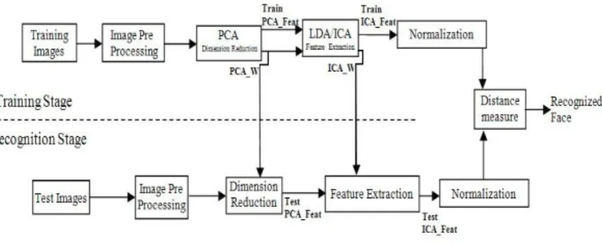
Human face detection and recognition is an active area of research spanning several disciplines such as image processing, pattern recognition and computer vision with wide range of applications such as personal identity verification, video-surveillance, facial expression extraction, advanced human and computer interaction. The wide-range variations of human face due to pose, illumination, and expression, result in a highly complex distribution and deteriorate the recognition performance. Hence, there is a need to develop robust face recognition algorithm. Block diagram of a typical face recognition system is shown in Fig. 1. In this, preprocessing is a filtering method used to reduce noise and dependence on precise registration.
Classification is usually one of a number of standard methods: common examples are minimum distance classifier and artificial neural networks, etc. Feature extraction is the area that tends to differentiate.This paper addresses the feature extraction method using gabor wavelets and PCA on face images. A good survey of face recognition system is found in [1]. The methods for face recognition can be divided into two different classes: geometrical features matching and template matching.
Figure 1. Block diagram of a typical face recognition system
In the first class, some geometrical measures about distinctive facial features such as eyes, mouth, nose and chin are extracted. With this extracted facial features, the recognition is done. In the second class, the face image is represented as a
two-∗Corresponding Author.
Email Address:[email protected]
Preprocessing Feature Extraction Classification
c
⃝2010 Published by Elsevier Ltd
Procedia Computer Science 2 (2010) 83–93
www.elsevier.com/locate/procedia
1877-0509 c⃝2010 Published by Elsevier Ltd doi:10.1016/j.procs.2010.11.011
Open access under CC BY-NC-ND license.
dimensional array of intensity values and this is compared to a single or several templates representing a whole face. The success of any face recognition method depends on the choice of the features used by the classifier. This feature selection method in a pattern recognition problem can be accomplished using a standard feature extraction method which extracts the features from the raw input data. By such methods the data used for processing are much reduced and also provide better discriminating ability.
The gabor filters used in the pre processing stage form a feature vector called gabor features of face images. Gabor transformed face images exhibit strong characteristics of spatial locality, scale, and orientation selectivity. These images can, thus, produce salient local features that are most suitable for face recognition. Face-based approach [2-6] attempts to capture and define the face as a whole image. The face is treated as a two-dimensional pattern of intensity variation. Under this approach, face is matched through identifying its underlying statistical regularities. One popular method for feature selection and dimensionality reduction is the Principle Component Analysis (PCA). Reconstruction of human faces using PCA was first done by Kirby and Sirovich [7] and recognition of human faces was done by Turk and Pentland [3]. The recognition method, known as eigenface method defines a feature space which reduces the dimensionality of the original data space. This reduced data space is used for recognition.
However, common PCA-based methods suffer from two limitations, namely, poor discriminatory power and large computational load. It is well known that PCA gives a very good representation of the faces. Given two images of the same person, the similarity measured under PCA representation is very high and given two images of different persons, the similarity measured will also be high, which means PCA representation gets a poor discriminatory power within the same class. The above short comings were overcome by adding LDA, which is one of the most important feature selection algorithms in appearance based methods [4]. But, to get a precise result, a large number of samples for each class is required. Due to the small sample size problem with LDA, a larger number of samples from each class is required. Hence, many LDA based approaches first use the PCA to project an image into a lower dimensional space or so called face space, and then perform the LDA to maximize the discriminatory power.
The second problem in PCA-based method is that it will de-correlate the input data using second order statistics, generating a compressed data with minimum mean squared projection error, but it will not account for the higher order dependencies in the input data projected onto them. To overcome this problem ICA is used which minimizes both second order and higher order dependencies in the input and attempts to find the basis along which the data (when projected onto them) are statistically independent[9]. ICA is used to reduce redundancy and represent independent features explicitly. These independent features are most useful for subsequent pattern discrimination and associative recall [11]. The extracted features from the test and the train sections are classified using Euclidean distance method.
In the proposed method, the frontal face images are gabor filtered and the vector representation of these filtered face image is reduced using PCA. The reduced principle feature vectors are used as input features for statistical models like LDA and ICA for extracting discriminant and independent feature vectors. These extracted features are normalized using UL and MV normalization methods. In comparison with the conventional use of PCA, the proposed method gives better recognition rate and discriminatory power with the use of statistical models. The algorithm is tested with the use ORL face database with 200 training and 200 test samples. The feasibility of the new algorithm has been demonstrated by experimental results. Also encouraging results are obtained with ICA method than LDA method using MV normalization technique.
This paper is organized as follows: Section 2 reviews the background of PCA and eigenfaces. Section 3 deals with the basics of Gabor wavelets and Gabor features. Section 4 deals with LDA. Section 5 details about ICA. Section 6 deals with the normalization methods. The proposed method is reported in section 7. Experimental results are presented in Section 8 and finally, Section 9 gives the conclusions.
2. Principal Component Analysis
The Principal Component Analysis (PCA) is one of the most successful technique that has been used for image compression and recognition .The purpose of PCA is to reduce the large dimensionality of the data space (observed variables) to a smaller intrinsic dimensionality of feature space (independent variables), which are needed to describe the data economically when there is a strong correlation between observed variables and independent variables [7]. PCA can transform each original image of the training set into a corresponding eigenface. An important feature of PCA is that one can reconstruct any original image from the training set by combining the eigenfaces, which are nothing but characteristic features of the faces. Therefore the original face image can be reconstructed from eigenfaces by summing up all the eigenfaces (features) in the right proportion. Each eigenface represents only certain features of the face, which may or may not be present in the original image. If the feature is present in the original image to a higher degree, the share of the corresponding eigenface is the “sum” of the eigenfaces should be greater and vice – versa. So, in order to reconstruct the original image from the eigenfaces, building a kind of weighted sum of all eigenfaces is required. That is, the reconstructed original image is equal to a sum of all eigenfaces, with each eigenface having a certain weight. This weight specifies, to what degree the specific feature (eigenface) is present in the original image. By using all the eigenfaces extracted from original images, exact reconstruction of the original images is possible. But for practical applications, certain part of the eigenfaces is used. Then the reconstructed image is an approximation of the original image. However losses due to omitting some of the eigenfaces can be minimized. This happens by choosing only the most important features (eigenfaces) [2].
The details are described in the following section:
2.1 Mathematics of PCA
A 2-D facial image can be represented as 1-D vector by concatenating each row (or column) into a long thin vector. 1. Assume the training sets of images represented by Г1, Г2, Г 3,…, Г m, with each image Г(x,y) where (x,y) is the size of the image represented by p and m is the number of training images. Converting each image into set of vectors given by (m x p). 2. The mean face Ψ is given by:
∑
=Γ
=
Ψ
m i im
11
(1)3. The mean-subtracted face is given by(Φi):
Ψ
−
Γ
=
Φ
i i (2)where i = 1, 2, 3….m. and сɌϭ͕ɌϮ͕͙͙Ɍŵ͕is the mean-subtracted matrix with size Amp͘ 4. By implementing the matrix transformations, the vector matrix is reduced by:
T pm mp
mm
A
A
C
=
×
(3)where C is the covariance matrix and T is the transpose matrix.
5. Finding the eigen vectors Vmm and eigen values λm from the C matrix and ordering the eigen vectors by highest eigen values. 6. With the sorted eigen vectors matrix, Φm is adjusted. These vectors determine the linear combinations of the training set images to form the eigen faces represented by Uk as follows
∑
=Φ
=
m n n kn kV
U
1 ͕Vkn , k = 1,2…..,m. (4)7. Instead of using m eigen faces, m′ eigen faces (m′<< m) is considered as the most significant eigen vectors provided for training of each individual.
8. With the reduced eigen face vector, each image has its face vector given by
(
Γ
−
Ψ
)
=
Tk
k
U
W
, k = 1,2,…., m′. (5)9. The weights form a feature vector given by
[
1,
2,...
m']
Tw
w
w
=
Ω
(6)10. These feature vectors are taken as the representational basis for the face images with reduced dimension. 11. The reduced data is taken as the input to the next stage for extricating discriminating feature.
3. Gabor Wavelet Theory
The prime motive behind the feature based approach is the representation of face image in a very compact manner and hence the memory used is reduced. This system gains its importance as the size of the database is increased. This feature based method aims to find the important local features on a face and represent the corresponding information in an efficient way. The selection of feature points and representation of those values has been a difficult task for a face recognition system. Physiological studies found that simple cells present in human visual cortex can be selectively tuned to orientation as well as spatial frequency. J.G.Daugman[12] has worked on this and confirmed that the response of the simple cell could be approximated by 2D Gabor filters.
Because of their biological relevance and computational properties, Gabor wavelets were introduced into the area of image processing [15,16]. The Gabor wavelets, whose kernels are similar to the 2D receptive field profiles of the mammalian cortical simple cells, exhibit desirable characteristics of spatial locality and orientation selectivity, and are optimally localized in the space and frequency domains.
One of the most successful face recognition method is based on graph matching of coefficients which are obtained from Gabor filter responses [13,14]. These matching methods have a drawback due to manual definition of training graphs, complexity in matching, etc. These drawbacks were overcome by Gabor wavelets. The Gabor wavelet is well known for its effectiveness to extract the local features in an image. It has the ability to exhibit the desirable characteristics of capturing salient visual properties such as spatial localization, orientation selectivity, and spatial frequency selectivity. This method is robust to changes in facial expression, illumination and poses. Applying statistical models like PCA, LDA, ICA to the Gabor filtered feature vector represents crisp gabor feature vectors. In order to consider all the gabor kernels, all the features were concatenated to form a single gabor feature vector. This high dimensional gabor vector space is then reduced using the PCA. Further on applying the ICA and LDA on the reduced data, the more discriminating features were obtained.
The Gabor wavelets (kernels, filters) can be defined as follows [12], [17], [18]:
( )
(
)
⎟⎟⎠
⎞
⎜⎜⎝
⎛
⎟⎟⎠
⎞
⎜⎜⎝
⎛
−
−
⎟
⎟
⎠
⎞
⎜
⎜
⎝
⎛
−
=
Ψ
22
exp
,
exp
2
,
exp
,
2 2 2 2 ,σ
ν
μ
σ
ν
μ
ν
μ
ν μik
z
z
k
k
z
(7)Where μ and v in Eqn. 7 define the orientation and scale of the Gabor kernels, z = (x,y) and ||.|| denotes the norm operator, and the wave vector k μ,v is defined as follows:
(
ν
)
ν ν
μ
=
k
i
Φ
k
,exp
(8)where kv = kmax /fv and φμ = πμ/8, kmax is the maximum frequency, and f is the spacing factor between kernels in the frequency
domain [18].
The Gabor kernels in Eq. 7 are all self-similar since they can be generated from one filter, the mother wavelet, by scaling and rotation via the wave vector kμ,v. Each kernel is a product of a Gaussian envelope and a complex plane wave, while the first term
in the square brackets in Eq. 10 determines the oscillatory part of the kernel and the second term compensates for the DC value. The effect of the DC term becomes negligible when the parameter σ, which determines the ratio of the Gaussian window width to wavelength, has sufficiently large values.
In most cases the use of gabor wavelets of five different scales, v
∈
{0,….., 4} and eight orientations, μ∈
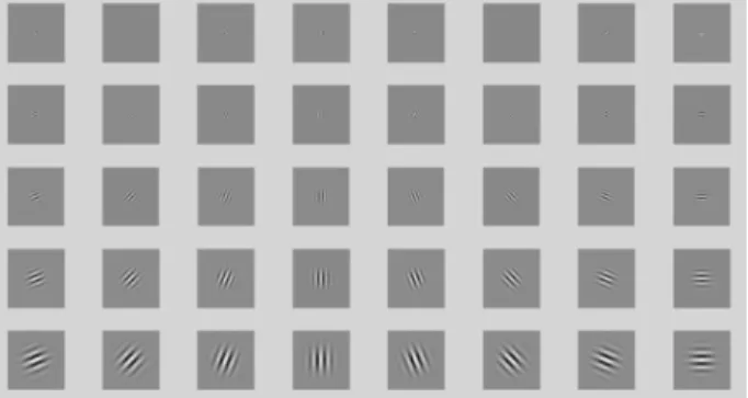
{0,…..,7}is used for representational bases[19]. Fig. 2 shows the Gabor kernels at five scales and eight orientations, with the following parameters: σ = 2π, kmax = π/2 and f= 2. The kernels exhibit desirable characteristics of spatial frequency, spatial locality, and orientation selectivity.3.1 Gabor Wavelet Representation
The Gabor wavelet representation of an image is the convolution of the image with a family of Gabor kernels as defined by Eq. 7. Let I(x,y) be the gray level distribution of an image, the convolution of image I and a Gabor kernel ψμ,v is defined as
follows.
( ) ( )
z
I
z
( )
z
O
μ,ν=
*
Ψ
μ,ν (9)where z = (x,y) and * denotes the convolution operator, and Oμ,v (z) is the convolution result corresponding to the Gabor kernel
at orientation μ and scale v. Therefore, the set S = {Oμ,v (z) , for μ
∈
{0,…..7} and v∈
{0,…..4}} forms the Gabor wavelet representation of the image I(z).Applying the convolution theorem, we can derive each Oμ,v (z) from Eq. 9 via the Fast Fourier Transform (FFT):
₣{ Oμ,v (z) } = ₣{I(z)} ₣{ ψμ,v(z)} (10)
Oμ,v (z) = ₣ -1
{ ₣ {I(z)} ₣ { ψμ,v(z)}} (11)
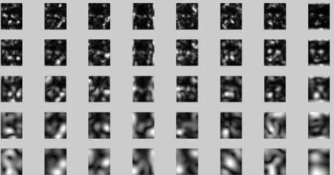
where ₣and ₣-1 denote the Fourier and inverse Fourier transform, respectively. Figs. 2 and 3 show the Gabor wavelet representation (the real part of gabor kernels with five scales and eight orientations and the magnitude of gabor kernels at five different scales). The input frontal face image as shown in Fig 4 is preprocessed using these kernels and the resultant convolution output of the image and the kernels are as shown in Fig. 5 (Real part of the convolution output of a sample image) and Fig. 6 (Magnitude of the convolution output of a sample image). To encompass different spatial frequencies (scales), spatial localities, and orientation selectivities, concatenate all these gabor representation results and derive an augmented feature vector X.
Figure 2. Gabor Kernels
Figure 3. Magnitude of Gabor Kernel at five different scales.
Figure 4. Sample frontal image
Figure 5. Real part of the convolution output of the sample image
Figure 6. Magnitude of the convolution output of the sample image
Before the concatenation, we first down sample each Oμ,v (z) by a factor ρ to reduce the space dimension. We then construct a
vector out of the Oμ,v (z) by concatenating its rows (or columns). Now, let Oρμ,v denote the normalized vector constructed from
Oμ,v (z) (down sampled by ρ), the augmented Gabor feature vector X(ρ) is then defined as follows:
X(ρ) = (O(ρ)t0,0 O(ρ)t0,1 ….. O(ρ)t4,7) (12)
where t is the transpose operator. The augmented gabor feature vector thus encompasses all the elements (down sampled ) of the Gabor wavelet representation set, S = { Oμ,v (z) : μ
∈
{0,…..7} , v∈
{0,…..4}} as important discriminating information. Fig. 3shows (in image form rather than in vector form) an example of the augmented Gabor feature vector, where the down sampling factor is 64, i.e. ρ = 64.
4. Linear Discriminant Analysis
Linear Discriminant Analysis (LDA) has been successfully used as a dimensionality reduction technique to many classification problem. The objective is to find a projection A that maximizes the ratio of between - class matrix Sb and against
within – class scatter Sw. Fisher Discriminant Analysis (FDA) based algorithms has a difficulty called small sample size problem (SSS) which exists in high dimensional pattern recognition tasks where the number of available samples is smaller than the dimensionality of the samples [20]. Due to this problem, many variants of the original FDA algorithm have been proposed for face recognition. Belhumeur and Hespanha [21] has proposed to perform PCA first before applying LDA in the PCA based subspace also known as PCA+LDA.
The LDA is defined by the transformation [22]
yi = W t
xi (13)
The columns of W are the eigenvectors of S-1w Sb , It is possible to show that this choice maximizes the ratio
det(Sb)/ det(Sw) (14)
These matrices are computed as follows:
(
)(
)
∑ ∑
= =−
−
=
c j n i T j j i j j i w jm
x
m
x
S
1 1 (15) where=
∑
n=j i j i jx
n
m
11
and
x
ijis the ith pattern of jth class, and nj is the number of patterns for the jth class. Then(
)(
)
∑
=−
−
=
∑
==
c j n i i T j j bx
n
m
m
m
m
m
S
1 11
,
.
(16)The eigenvectors of LDA are called “fisherfaces”. LDA transformation is strongly dependent on the number of classes (c), the number of samples (m), and the original space dimensionality (d). It is possible to show that there are almost c-1 nonzero eigenvectors. c-1 being the upper bound of the discriminant space dimensionality. We need d+c samples at least to have a nonsingular Sw [22]. It is impossible to guarantee this condition in many real applications. Consequently, an intermediate transformation is applied to reduce the dimensionality of the image space. To this end, we used the PCA transform. LDA derives a low dimensional representation of a high dimensional face feature vector space. From Eqn. 15 and Eqn. 16, the covariance matrix C is obtained as follows
C = Sw -1
* Sb (17)
The coefficients of the covariance matrix gives the discriminating feature vectors for the LDA method. The face vector is projected by the transformation matrix WLDA. The projection coefficients are used as the feature representation of each face image. The matching score between the test face image and the training image is calculated as the distance between their coefficients vectors. A smaller distance score means a better match. For the proposed work, the column vectors wi (i = 1,2…c-1) of matrix W are referred to as fisherfaces.
5. Independent Component Analysis
The problem in PCA-based method is that it will decorrelates the input data using second order statistics, generating a compressed data with minimum mean squared projection error. But it will not account for the higher order dependencies in the input and attempts to find the basis along which the data is projected onto them. To overcome this problem, ICA is used which minimizes both second order and higher order dependencies in the input and attempts to find the basis along which the data (when projected onto them) are statistically independent[24,25]. ICA of a random vector searches for a linear transformation which minimizes the statistical dependence between its components [26]. The principle feature vectors of the frontal image is obtained using PCA as given in Eqn. 6. This principle components are used as the input for the ICA and the most independent features are obtained[9]. Since it is difficult to maximize the independence condition directly, all common ICA algorithms recast the problem to iteratively optimize a smooth function whose global optima occurs when the output vectors U are independent . Thus use of PCA as a pre-processor in a two-step process allows ICA to create subspaces of size m by m. In [27], it is also argued that pre-applying PCA enhances ICA performance by (1) discarding small trailing eigenvalues before whitening (linear transformation of the observed variable) and (2) reducing computational complexity.
Let the selected principle features be the input to ICA as given in Eqn. 6. i.e Ω be of the size m by z, containing the first m eigenvectors of the face database. The rows of the input matrix to ICA are variables and the columns are observations, therefore, ICA is performed on ΩT. The m independent basis images in the rows of U are computed as
U = W * ΩT (18)
where W is the weight matrix from the PCA. Then, the n by m, ICA coefficients matrix B for the linear combination of independent basis images in U is computed as follows
Let C be the n by m matrix of PCA coefficients. Then,
C = I*Ω and I = C * ΩT (19) From U = W* ΩT and the assumption that W is invertible,
ΩT = W-1* U (20)
Therefore,
I = (C* W-1 )* U
I = B * U (21)
Each row of B contains the coefficients for linearly combining the basis images to comprise the face image in the corresponding row of I. Also, I is the reconstruction of the original data with minimum squared error as in PCA.
6. Normalization Method
The characteristics of the extracted features depends on the approach employed for the feature extraction as well as on the procedure used to normalize the extracted feature vectors. Here two different normalization methods have been used to normalize the extracted features [28].
6.1 Unit Length Normalization - UL
Unit length normalization (UL) scales all of the components of the input x accordance with the following expression to produce the normalized feature vector xi
x
x
X
i i=
* , i = 1,2,3….. n. (22) where n is the total population,.
denotes the norm operator and Xi* stands for the ith component of the normalized vector xi.6.2 Zero-Mean And Unit-Variance Normalization – MV
Using the same notation for the original and normalized feature vector as in the previous subsection, we can define the zero-mean and unit-variance normalization (MV) technique as follows:
σ
−
μ
=
i ix
X
* , i = 1,2,3….. n (23)where μ denotes the mean value of the feature vector x and σ represents its standard deviation. the MV technique transforms the feature vector x to a random variable with a mean value of zero and variance of one.
7. Proposed Method
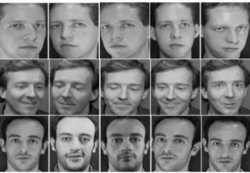
The block diagram of the proposed face recognition system is as shown in Fig. 7. This proposed work uses the ORL database acquired at the Olivetti Research Laboratory in Cambridge, U.K. The database is made up of 400 face images that correspond to 40 distinct subject. Thus, each subject in the database is represented with 10 facial images that exhibit variations in terms of illumination, pose and facial expression. The images are stored at a resolution of 92 × 112 and 8-bit grey levels. Out of this 400
frontal images, 200 images (5 from each class) were considered for training and the remaining 200(remaining 5 from each class) were used for testing. Figs. 8&9 show the scaled training and test samples.
Figure 7. Block diagram of the proposed face recognition system
The system follows the face based approach and it consists of two stages namely the training and the recognition stage. In the training stage, gabor wavelet is used in the preprocessing stage which is robust to changes in illumination, pose and expression. To facilitate the Gabor wavelet representations, the ORL images are scaled to 128x128 using a bicubic interpolation. The gabor kernels as defined in Eqn. 7 uses five different scales and eight orientations which results in 40 different filters. The input image is convoluted with the gabor kernel and the convoluted real and magnitude responses are shown in Fig. 5 and 6 respectively. This convoluted feature vector is then down sampled by a factor of ρ = 64. To encompass all the features produced by the different Gabor kernels, the resulting Gabor wavelet features are concatenated to derive an augmented Gabor feature vector.
The resulting high dimension gabor feature vector is taken as input to the next stage. This stage uses the PCA for reducing the dimension of the feature vector and extract the principle features. Here the eigen vectors were calculated, sorted in the ascending order and the top eigen vectors (n-1) are used for representation of feature vectors (PCA_Feat). Also the weight matrix is computed as PCA_W. This eigen projection is then used as input to the next stage of ICA using the FastICA algorithm. The algorithm takes the projected data and gives the independent features ICA_Feat and the independent weight matrix ICA_W. This is used to find the test ICA features.
The same procedure is applied for feature extraction using LDA. Here using PCA_Feat is used as input to the LDA block. The between class (Sb) and within class scatter matrix (Sw) is obtained using this projection matrix. LDA gives the projected weight matrix LDA_W, which is used to find the LDA test features. These extracted features are normalized using UL and MV techniques.
Figure 9. Scaled test samples.
In the recognition stage, the test samples are preprocessed as done in the training stage. The test image matrix is multiplied with PCA_W and this results in test PCA features(PCA_test). This PCA_test when convoluted with ICA_W gives the test features(ICA_test). The same procedure is used to obtain the test features for LDA method(LDA_test and LDA_W). The classification stage uses Euclidean distance method. Here the training and test feature vectors are considered. For a given sample image, test feature vector is found and the distance between this test feature vector and the all the training feature vectors are calculated. From the distance measure, the index with minimum distance represents the recognized face from the training set.
8. Results and Discussion
ORL Face database are tested at four different experimental setups as listed below. 1. PCA alone.
2. Gabor with PCA. 3. Gabor with PCA and LDA.
ϰ͘
Gabor with PCA and ICA.Classification technique used is the Euclidean distance measure for the above said four methods. Also the UL and MV method of normalization were considered. The number of features considered for recognition is varied and the corresponding recognition rate is given. The successfulness of the proposed method is compared with some popular face recognition schemes like Gabor wavelet based classification [8], the PCA method [29], the LDA method [30], and the eigen faces method[3].
Table 1. Comparison Of Recognition Rate
Algorithm Normalization Method
Number of Features
40 50 66 100 199
PCA alone Conventional 89 90 90 90.5 91
UL 87 87.5 88 89 91.5
MV 92.5 92.5 93.5 93.5 93.5
Gabor with PCA Conventional 83 84 87.7 92 93
UL 83.5 83.5 86 90 92.5
MV 89 90.5 92 93 94
Gabor with PCA and LDA Conventional 84 86 90 92 92.5
UL 90 90.5 92 92.5 93
MV 90.5 91.5 93 93 94.4
Gabor with PCA and ICA Conventional 88 89 89 89.5 95
UL 91.6 93 93 93.5 94.5
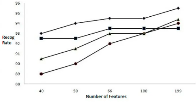
Fig. 10 shows the recognition performance for the four methods with MV normalization. The minimum number of features selected for the proposed technique is 40.
Figure 10. Performance comparison with MV normalization
9. Conclusion
In this proposed work, a gabor feature based method is introduced for face recognition system. For different scales and orientations of the gabor filter, the feature vectors were formulated. Using PCA, these feature vector, dimension is reduced followed by feature extraction is done using ICA and LDA. The extracted features are normalized using UL and MV normalization techniques. ED method is used for the classification. From the simulation results, it has been found that the recognition rate for the selected database is high with features extracted from ICA based gabor methods than with LDA and simple PCA methods. This recognition rate is obtained with fixed number of PCA features. The comparison of recognition rate for all the four methods is tabulated in Table. 1. This shows recognition rate for selection of ICA/LDA features in the case of PCA features equal to 40, 50, 66, 100, 199. It is noted that features based on ICA based method following MV normalization technique gives better recognition rate. From the results, it is obvious that as the number of features selected in PCA/ICA/LDA increase, the recognition rate also increases. But this in turn increases the computational load. It has been clear that normalization of the extracted features will get a better recognition rate and ensures an increase in the by 5% when compared to the feature vectors without normalization.
References
[1] W. Zaho, R.Chellappa, P.J.Philips and A.Rosenfeld, “Face recognition A literature survey,” ACM Computing Surveys, Vol. 35, No. 4, pp. 399– 458, December 2003.
[2] M. Kirby and L. Sirovich, “ Application of the Karhunen - Loeve procedure for the characterization of human faces,” IEEE Trans. PAMI., vol. 12, 103-108, 1990.
[3] M. Turk and A. Pentland, “Eigenfaces for recognition,” J. Cognitive Neuroscience,vol. 3, 71-86., 1991.
[4] D. L. Swets and J. J. Weng, “Using discriminant eigenfeatures for image retrieval”, IEEE Trans. PAMI., vol. 18, No. 8, 831-836, 1996.
[5] D. Valentin, H. Abdi, A. J. O'Toole and G. W. Cottrell, “Connectionist models of face processing: A Survey”,J. Pattern Recognition, vol. 27,1209- 1230, 1994.
[6] 6. M V. Wickerhauser, “ Large - rank approximate component analysis with wavelets for signal feature discrimination and the inversion of complicated maps”, J. Chemical Information and Computer Sciences, vol. 34, No.5,1036- 1046, 1994.
[7] M. Kirby and L. Sirovich, “Application of the karhunenloeve procedure for the characterization of human faces”, IEEE Trans. Pattern Analysis and Machine Intelligence, vol. 12, No 1, 103–108, 1990.
[8] A. J. O'Toole, H. Abdi, K. A. Deffenbacher and D. Valentin, “A low- dimensional representation of faces in the higher dimensions of the space”, J. Opt. Soc. Am., A, vol. 10, 405-411, 1993.
[9] P. Belhumeur J. P. Hespanha and D. J. Kriegman, “Eigenfaces vs. Fisherface; Recognition using class specific linear projection”, Pattern Recognition and Machine Intelligence, vol. 17, Vol 9, pp. 711-720, 1997.
[10]M.S. Bartlett, J.R. Movellan, and T.J. Sejnowski, “Face recognition by independent component analysis”, IEEE Trans Neural Networks, 13, 1450–1464, 2002.
[11] Chengjun Liu, and Harry Wechsler, “Independent Component Analysis of Gabor Features for Face Recognition”, IEEE Transactions on Neural Networks, vol. 14, NO. 4, 919-928, 2003.
[12] J. G. Daugman, “Two dimensional spectral analysis of cortical receptive field profile”, Vision Research, vol. 20, pp. 847-856, 1980.
[13] P. Phillips, “The FERET database and evaluation procedure for face recognition algorithms”, Image and Vision Computing, vol. 16, no. 5, pp. 295-306, 1998.
[14] L. Wiskott, J. M. Fellous, N. Krüger and Christoph von der Malsburg, “Face Recognition by Elastic Graph Matching,” In Intelligent Biometric Techniques in fingerprint and Face Recognition, CRC Press, Chapter 11, pp. 355-396, 1999.
[15] J.G. Daugman, “Complete discrete 2-d Gabor transforms by neural networks for image analysis and compression,” IEEE Trans. Pattern Analysis and Machine Intelligence, vol. 36, no. 7, pp. 1169–1179, 1988.
[16] J. Jones and L. Palmer, “An evaluation of the two-dimensional Gabor filter model of simple receptive fields in cat striate cortex,” J. Neurophysiology, pp. 1233–1258, 1987.
[17] S. Marcelja, “Mathematical description of the responses of simple cortical cells,” Journal Opt. Soc. Amer., vol. 70, pp. 1297–1300, 1980.
[18] M. Lades, J.C. Vorbruggen, J. Buhmann, J. Lange, C. von der Malsburg, Wurtz R.P., and W. Konen, “Distortion invariant object recognition in the dynamic link architecture,” IEEE Trans. Computers, vol. 42, pp. 300–311, 1993.
[19] D. Field, “Relations between the statistics of natural images and the response properties of cortical cells,” J. Opt. Soc. Amer. A, vol. 4, no. 12, pp. 2379– 2394, 1987.
[20] Chen, L.F., M.L. Hong-Yuan, K. Ming-Tat, L. Ja-Chen and Y. Gwo-Jong, “A new LDAbased face recognition system which can solve the small sample size problem”, Pattern Recognition, vol 33, pp 1713-1726, 2000
[21] Belhumeur, P.N., J.P. Hespanha and D.J. Kriegman, “ Eigenfaces vs. Fisherfaces: recognition using class specific linear projection”, IEEE Trans. Pattern Anal. Mach. Intelligence, vol 19, pp. 711-720, 1997
[22] Vitomir Struc, Nikola pavesi, “Gabor-Based Kernel Partial-Least-Squares Discrimination Features for Face Recognition”, Informatica, vol. 20, No. 1, 115– 138, 2009.
[23] Pierre A. Devijver and Josef Kittler, “Pattern Recognition: A statistical Approach,” Prentice-Hall,Englewood Cliffs, N.J., 1982.
[24] M.S. Bartlett, J.R. Movellan, and T.J. Sejnowski, “Face recognition by independent component analysis”, IEEE Trans Neural Networks, vol 13, 1450– 1464, 2002.
[25]Kresimir Delac, Mislav Grgic, Sonja Grgic , “Independent comparative Study of PCA, ICA, and LDA on the FERET Data Set”, Wiley periodicals, vol 15, pp. 252-260, 2006.
[26] P. Comon, “Independent component analysis, a new concept?,” Signal Processing, vol. 36, pp. 287–314, 1994.
[27] C. Liu and H. Wechsler, Comparative Assessment of Independent Component Analysis (ICA) for Face Recognition, presented at International Conference on Audio and Video Based Biometric Person Authentication, Washington, DC, 1999.
[28] V. Struc, N. Pavesic, “A comparison of feature normalization techniques for pca-based palmprint recognition”.
[29] M. H. Yang, N. Ahuja, and D. Kriegman, “Face recognition using kernel eigenfaces,” Proc. IEEE Int. Conf. Image Processing, 2000.
[30] A. Hossein Sahoolizadeh, B. Zargham, “A New feace recognition method using PCA, LDA and Neural Networks”, proceedings of word academy of science, Engineering and Tech, vol. 31, July 2008.