Solution Path Clustering with Robust Loss and Concave Penalty

(1)

UC Riverside

UC Riverside Electronic Theses and Dissertations

Title

Permalink

https://escholarship.org/uc/item/6kk6628s

Author

Schuberg, Edward

Publication Date

2019 Peer reviewed|Thesis/dissertation

(2)

UNIVERSITY OF CALIFORNIA RIVERSIDE

Solution Path Clustering with Robust Loss and Concave Penalty

A Dissertation submitted in partial satisfaction of the requirements for the degree of

Doctor of Philosophy in Applied Statistics by Edward Schuberg March 2019 Dissertation Committee:

Dr. Weixin Yao, Co-Chairperson Dr. Shujie Ma, Co-Chairperson Dr. Wenxiu Ma

(3)

Copyright by Edward Schuberg

(4)

The Dissertation of Edward Schuberg is approved:

Co-Chairperson

(5)

Acknowledgments

I am grateful to my advisors, Dr. Weixin Yao and Dr. Shujie Ma. Their patient guidance has been invaluable, with many important lessons both inside and outside the world of statistics. I would also like to thank Dr. Wenxiu Ma for her time, support, and good will throughout the committee process. I am grateful to Dr. Daniel Jeske whose men-torship and outreach completely changed the trajectory of my professional life. Finally, I am grateful to my undergraduate advisor, Dr. David Andrews, without whose encouragement I would not be here. Encouragement is a hard thing to overestimate.

(6)

(7)

ABSTRACT OF THE DISSERTATION

Solution Path Clustering with Robust Loss and Concave Penalty by

Edward Schuberg

Doctor of Philosophy, Graduate Program in Applied Statistics University of California, Riverside, March 2019

Dr. Weixin Yao, Co-Chairperson Dr. Shujie Ma, Co-Chairperson

The main purpose of this dissertation is to demonstrate that using a robust loss function (instead of the usual least squares loss) improves the clustering quality in the solution path clustering scheme. Cluster analysis simultaneously attempts to determine the number of clusters and estimate cluster location and membership. Convex clustering, distinguishing itself from other popular clustering methods, casts the clustering objective as a convex optimization problem and thus admits a global solution. It is a useful exploratory technique which outputs a solution path, evoking the name, “solution path clustering.” The solution path is a tree-like structure with cluster results ranging from n clusters down to

a single cluster. Now, the benefits of convex clustering come at a cost since the use of a convex penalty can seriously bias the results and ruin the search for good cluster results. To lessen the bias, Ma and Huang (2017) proposed concave penalties to form the cluster centers. While the clustering objective is no longer convex, the quality of the solutions is improved.

(8)

func-tions instead of the usual least squares loss. Following Ma and Huang (2017), we also use a concave penalty to form clusters. The robust loss and concave penalty work together to mitigate the influence of outliers and minimize bias in the estimation of cluster locations, especially when the true distance between clusters is large. We introduce the IRLS-ADMM algorithm to minimize our proposed objective function and prove its convergence to a local minimum. Any loss function that admits an IRLS formulation or a majorizing surrogate can be used. We also study asymptotic and oracle properties of the estimator. Finally, we demonstrate the performance of our proposed method through simulation experiments and on real data sets, as well as provide some preliminary results on choosing the number of clusters via the modified BIC (Wang, Li, and Leng, 2009).

(9)

List of Figures

1.1 K-means example with K = 2 and K= 3 . . . 6

1.2 Example dendrogram of hierarchical clustering . . . 11

2.1 Solution path plots illustrating effect of post-processing step. . . 19

2.2 Solution path plots illustrating effect of different Gaussian weight choices. . 20

2.3 Solution path plots illustrating effect of different weight choices. . . 22

2.4 Plot of MCP penalty with different values of the concavity parameter ω. . . 24

2.5 Solution path plot with MCP penalty. . . 25

2.6 Different weights effects on recovery of true clusters. . . 27

3.1 Comparing solution path plots using least squares loss and robust loss with outlier present. . . 42

3.2 Plots of h(x),h(√x), andw(x) for the Huber and Tukey functions. . . 47

3.3 Histograms for Side Noise and Inside Noise with n= 200. . . 96

3.4 Dotplot of President Dataset from Hayden (2005). . . 104

3.5 Solution path plots for the President Dataset. . . 105

4.1 Untransformed data vs. Transformed Data . . . 111

4.2 Scatter plots of settings 1 and 5. . . 118

4.3 Scatter plots of noise dimension settings withn= 200. . . 122

4.4 Scatter plots of the Pi Letter and Mickey Mouse settings with n= 200. . . 125

4.5 Scatter plots of the correlation settings with n= 200. . . 129

4.6 Plot of Fisher’s Iris dataset. . . 132

4.7 Plot of the two greatest principle components of the Seeds dataset. Taken from Charytanowicz, et al. (2010) . . . 135

(12)

List of Tables

3.1 Solution path clustering performance results with various loss functions, cor-responding to simulation settings 1-5 for n= 40. . . 89 3.2 Solution path clustering performance results, averaged across 200 replicates,

with various loss functions, corresponding to simulation settings 1-5 forn= 200. 90 3.3 Solution path clustering performance results with various loss functions,

cor-responding to simulation settings 6-10 for n= 200. . . 91 3.4 BIC results for simulation settings 1-5 forn= 40 and 200 replicates. . . 92 3.5 BIC results for simulation settings 1-5 forn= 200 and 200 replicates. . . . 93 3.6 BIC results for simulation settings 6-10 forn= 200 and 200 replicates. . . . 94 3.7 Solution path clustering performance results with various loss functions,

cor-responding to simulation settings 1-6 for n= 50. . . 99 3.8 Solution path clustering performance results with various loss functions,

cor-responding to simulation settings 1-6 for n= 200. . . 100 3.9 BIC results for simulation settings 1-6 forn= 50. . . 101 3.10 BIC results for simulation settings 1-6 forn= 200. . . 102 3.11 Number of clusters chosen by the modified BIC with different c values for

the President Data Set. . . 105 4.1 Solution path clustering results for settings 1-7 withn= 200. . . 119 4.2 BIC results for settings 1-7 with n= 200 and 100 replicates. . . 120 4.3 Solution path clustering results for noise dimension settings with n= 200. . 123 4.4 BIC results for noise dimension settings with n= 200 and 100 replicates. . . 123 4.5 Solution path clustering results for the Pi Letter and Mickey Mouse settings

withn= 200. . . 126 4.6 BIC results for the Pi Letter and Mickey Mouse settings with n= 200 and

100 replicates. . . 126 4.7 Solution path clustering results for the correlation settings withn= 200. . . 130 4.8 BIC results for the correlation settings with n= 200 and 100 replicates. . . 130 4.9 Number of clusters chosen by the modified BIC with different c values for

the Iris Data Set. . . 133 4.10 Copied Table 1 from Charytanowicz, et al. (2010) to compare Complete

(13)

4.11 Summary results for the Seeds dataset to compare Huber Approximation to Absolute Loss to the Least Squares Loss in Solution Path Clustering. . . 136 4.12 Number of clusters chosen by the modified BIC with different c values for

(14)

Chapter 1

Introduction to Clustering

Clustering is a fundamental and challenging problem in many applications. The goal is to partition the data into homogeneous subgroups in a relevant and meaningful way without any prior knowledge of the structure of the data. This makes cluster analysis a type of unsupervised learning. The data is believed to be coming from a population that is composed of several distinct sub-populations which we wish to detect. Clustering meth-ods are comprised of fundamental techniques used in statistics, machine learning, pattern recognition, as well as in many applied fields. Understood loosely, clustering is essentially “the practice of classifying objects according to perceived similarities [and] is the basis for much of science” (Jain and Dubes, 1988).

There are many books on clustering, such as Hartigan (1975), Jain and Dubes (1988), Kaufman and Rousseeuw (1990), Gordon (1999), and Everitt et. al. (2011). Xu and Wunsch (2005) also provide an excellent survey of clustering algorithms. Clustering also has many applications in a variety of fields. Banerjee and Ghosh (2001) use cluster analysis

(15)

on click-stream patterns on websites to generate customized user content. Tzanetakis and Cook (2002) use clustering for the classification of musical genres. Dolan and Van der Maas (1998) discuss mixture models in the structural equation modeling context. Ma and Huang (2016) discuss subgroup analysis for personalized medicine and treatment decisions. Schork, Allison, and Thiel (1996) discuss mixture models to assess the impact of possible underlying genotypes, where order selection is key in the identification of the existence of major genes and whether or not they are dominant. Chen and Maitra (2011) discuss cluster analysis with an application to mutual funds.

Interestingly, the human eye can quite naturally and rapidly identify groupings and clusters in a two dimensional scatter plot. However, the need to systematically define how to form clusters and how many clusters to form becomes apparent in order to generalize to higher dimensional data. This also solves the problem when different people identify (justifiably) different groupings in the data. In Everitt (1974), a few definitions of a cluster are offered:

1. “A cluster is a set of entities which are alike, and entities from different clusters are not alike.”

2. “A cluster is an aggregation of points in the test space such that thedistance between any two points in the cluster is less than the distance between any point in the cluster and any point not in it.”

3. “Clusters may be described as connected regions of a multi-dimensional space con-taining a relatively high density of points, separated from other such regions by a region containing a relatively low density of points.”

(16)

These three definitions offer a guide in specifying mathematically the clustering objective. For example, one might classify a set of entities to be “alike” if the “distance” (such as Euclidean distance) between two points is small enough (below some threshold).

Ultimately, cluster analysis must address two fundamental questions:

Question 1. How do we form the clusters?

Question 2. How many clusters is optimal?

Question 2 is challenging in its own right, but it also very much hinges upon a good answer to Question 1. In other words, a sensible clustering method (e.g. an appropriately specified mixture of normals) will help answer Question 2. On the other hand, if a clustering method performs poorly, any number clusters, even if optimal, will not yield a sensible partition of the data. The issue become even more mystifying since it is unclear how to define what the “optimal” number of clusters should be. It also depends on what the goal is for performing the cluster analysis. For example, the goal may be to confirm that a certain grouping exists among a set of observations, or the cluster partition may become the grounds for the design of an experiment.

Solution Path Clustering, as opposed to K-means clustering or model-based

clus-tering, does not require the number of components (clusters) to be specified beforehand. While this partially obviates the need to select the number of clusters, we offer a selec-tion method using modified BIC in an attempt to address this difficult issue. Thus, this project seeks to contribute to the literature which tries to resolve the two intimately linked clustering principles enumerated in Questions 1 and 2.

(17)

It reviews K-means clustering and hierarchical clustering which are, in some sense,

pre-cursors to convex clustering and Solution Path Clustering. It also reviews clustering based on finite mixture models. While mixture models present some challenges in implementa-tion, they offer a clean theoretical framework to classify observations. They also bear some resemblance to K-means clustering. The chapter concludes with a survey of methods for

selecting the number of clusters.

1.1 K

-means Clustering

K-means clustering is perhaps the most well-known clustering method. It remains

one of the most popular methods due to its simplicity and fast implementation. To employ theK-means methods, the user specifies beforehand the number of clusters. The objective

is then to minimize the within-cluster sum of squares for that fixed number of clusters. The following presentation of the K-means method follows closely to that of

Lind-sten, Ohlsson, and Ljung (2011). Let y1, y2, . . . , yn be observations in Rd. Let K be the fixed number of clusters that is specified beforehand. Let Gj ⊂ {1,2, . . . , n} be index sets

such that

Gj∩Gj0 =∅for each j6=j0 and

K

[

j=1

Gj ={1,2, . . . , n}

where∅denotes the empty set. Thus,i∈Gj means thatyi belongs to the j-th cluster. Let

G={G_j}K

j=1, and let ·

denote the Euclidean norm. Let card G_j denote the cardinality

(18)

given by min G K X j=1 X i∈Gj y_i−µ_j 2 such that µj = 1 cardGj X i∈Gj yi and K [ j=1 Gj ={1,2, . . . , n} (1.1)

Implementing an algorithm to solve this optimization problem is straightforward in most software packages. For example, the function “kmeans()” in R performs K-means

with four algorithms to choose from. Multiple algorithms have been proposed to solve the problem (1.1). Though the task is quite easy to state and conceptualize, it is quite difficult to find the most optimal solution. For example, convergence to a local minimum may produce odd results. This problem is worsened by the fact that the algorithms are known to be sensitive to the initial value (Pe˜na, Lozano, and Larra˜na 1999; see also Figure 1 in Lindsten, Ohlsson, and Ljung, 2011). This issue is often addressed by starting the algorithm from multiple initial values and then selecting the best solution. Another drawback to the algorithm is that it can be slow to converge (Vattani 2009). However, for the majority of datasets, the K-means algorithms are quite fast to converge and do not require many

iterations.

The simplicity of the K-means method proves to be perhaps its biggest weakness.

Firstly, the number of clusters, K, must be chosen and fixed beforehand. If K is chosen

badly (choosing K large when it should be small, or choosing K small when it should be

large), the results may be poor. Thus, practitioners often run K-means along a sequence

(19)

Secondly, the simplicity of the model is quite inflexible and has trouble accommo-dating more exotic datasets. The model implicitly assumes that the clusters are spherical and with the same variance. Thus, datasets exhibiting correlation may be difficult to clus-ter using the K-means method. The assumption that the clusters have the same variance

implies that they are of similar size to one another. In other words, assigning observations to its closest cluster is regarded as the best assignment since it does not take into account the cluster variance. This assumption equal variances across both clusters and dimensions can be unrealistic and lead to unsatisfactory results (e.g. one could try running k-means

withk= 3 on a Mickey mouse dataset where the ears are much smaller than the head. Part

(a)K-means withK= 2. (b)K-means withK= 3.

Figure 1.1: There are 150 total observations with 50 generated from each of N µ =

(0,0),Σ = I, N µ = (5,−2),Σ = I, and N µ = (5,2),Σ = I. The R function “kmeans()” was used with Lloyd’s algorithm.

(20)

of the head will end up getting assigned to the ears).

1.1.1 Convexifying k-means

The lack of being guaranteed the global solution to the k-means problem (1.1)

motivates a convexification. If thek-means task (1.1) can be somehow relaxed to a convex

problem, then the global solution can be realized. Consider first the optimization problem

min µ n X i=1 ky_i−µik2

such that{µ1, µ2, . . . , µn} containskunique vectors.

(1.2)

Hence, we shifted the problem from using k centroids to allowing a µi parameter for each

observation yi, so long as there are only k unique µi values. That an optimal solution of

(1.2) corresponds to an optimal solution of (1.1) is proved in Proposition 2 of Lindsten, Ohlsson, and Ljung (2011). We now need to express the constraint in (1.2) using formal mathematical notation. Thus, we need to count the number of unique vectors in a given set {µ1, µ2, . . . , µn}.

Define δj to be the number of µ0is where µj = µi, for i < j and j = 2,3, . . . , n.

Written mathematically, we haveδj =j−1−kγjk0where the vectorsγj = γ₁j, γ₂j, . . . , γ_jj₌₁

have elementsγ_ij =p(µi, µj). Here,p(µi, µj) is a non-negative, symmetric (penalty) function

that equals zero if and only ifµi =µj. Consider the vector δ= (δ2, δ3, . . . , δn). Notice that

kδk0 gives the number of times out ofn−1 trials that a µj, j = 2,3, . . . n, was not unique

compared to the all the µi, i = 1,2, . . . , j −1. In other words, the vector µj is unique

(compared to theµi that came before it) only if δj = 0. We can thus count the number of

(21)

1. We start with one cluster. We always have at least one cluster, which is why we only calculateδj starting atj = 2,3, . . . , n.

2. For j = 2,3, . . . , n, if δj = 0, increase our count of the number of clusters by 1. If

δj >0, leave the number of clusters unchanged.

It follows that the number of clusters (the number of unique vectors in{µ1, µ2, . . . , µn}) is

n− kδk0. We can hence formulate (1.2) as

min µ n X i=1 ky_i−µik2 such thatk=n− kδk0. (1.3)

Lindsten, Ohlsson, and Ljung (2011) state that, “In some sense, the convex function closest to theL0norm is the L1norm.” They relax thek-means criterion by replacing theL0 norm

with theL1 norm twice. Firstly, we change the constraint in (1.3) to k=n− kδk1 =n− n X j=2 |δj| =n− n X j=2 j−1− kγ j_k 0 =n− n X j=2

j−1− kγjk0 (since it’s always non-negative)

=n− n(n−1) 2 − n X j=2 kγjk0 = 3n−n 2 2 − n X j=2 kγjk0.

(22)

Problem (1.3) has now been transformed to min µ n X i=1 kyi−µik2 such that n X j=2 kγjk0 = 3n−n2 2 −k. (1.4)

We again replace theL0 norm used here to theL1 norm. This transforms the constraint to

3n−n2 2 −k= n X j=2 γj =X i<j γ_ij =X i<j p(µ_i, µ_j) =X i<j

p(µi, µj). (since the terms are non-negative)

If the function p(·,·) is chosen appropriately, then we will have successfully arrived to a convex problem: min µ n X i=1 kyi−µik2 such that X i<j p(µi, µj) = 3n−n2 2 −k. (1.5)

For example, we may usep(µi, µj) =kµi−µjkq forq ≥1. The final step in this development

is to use the equivalent Lagrangian formulation of (1.5) which is a much more convenient optimization problem: min µ n X i=1 ky_i−µik2+λ X i<j p(µi, µj). (1.6)

The book from Boyd and Vandenberghe (2004) contains a wealth information on convex analysis, including Lagrangian dual formulations. It can be shown, for example, that there

(23)

exists a λ > 0 such that (1.6) is equivalent to (1.5). However, the exact λ values are not

so important since λ can be interpreted as a regularization parameter which controls the

trade-off between the goodness-of-fit and the number of clusters.

1.2 Hierarchical Clustering

Hierarchical clustering, as the name suggests, builds a hierarchy of cluster solu-tions ranging from nclusters, where each data point is its own cluster, to a single cluster

consisting of all the data points. Hierarchical clustering can be agglomerative or divisive. Agglomerative clustering begins with clusters as as singleton points which are successively merged in stages until there is only a single cluster of all points. Divisive clustering begins from the opposite direction, starting with all points in a single cluster. Clusters are then split in consecutive stages until each cluster consists of only one data point. We focus here on agglomerative clustering, following the presentation found in Hocking et. al. (2011).

Let X ∈ Rn×d be the observed data matrix where the rows in X are the obser-vations of dimension d. The agglomerative scheme for hierarchical clustering suggests the

following optimization problem:

min M∈_Rn×d 1 2 X−M 2 F subject to X i<j 1Mi6=Mj ≤t. (1.7) Here, ·

F represents the Frobenius norm, Mi is the i-th row of M, and 1Mi6=Mj = 1 if

Mi 6=Mj and equals zero otherwise. Note that P_i<j =Pn_i₌₁Pn_j₌_i₊₁ sums over the n₂

=

n(n−1)/2 pairs of data points. When t≥ n₂

(24)

andMi =Xi for alliso that each data point is its own singleton cluster. Whent= n₂

−1, then one pair, (Mi, Mj), will be forced to merge. This is the first step in the agglomerative

scheme of hierarhical clustering. As tis sequentially decreased, more and more pairs of the

clusters will be merged until finally there is only a single cluster. Note that, in general, the

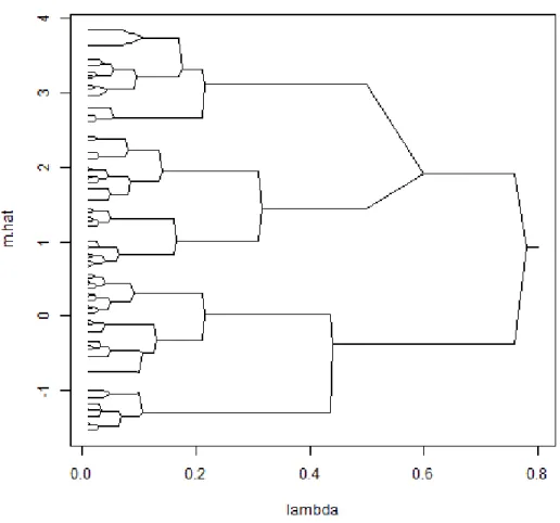
Figure 1.2: Dendrogram of an agglomerative hierarchical clustering scheme using squared Euclidean distance and single linkage. There are 40 observations with 20 generated from each ofN(µ= 1, σ= 1) andN(µ= 4, σ= 1). The R function “hclust()” was used.

(25)

task of finding the best pair of clusters to merge at each step is a difficult combinatorial problem. See Murtagh and Contreras (2011) for a recent review of agglomerative clustering algorithms and how they are implemented efficiently.

Note that the problem (1.7) is only one such formulation of hierarchical clustering. There are, in fact, many options that one may choose which govern how the clustering is performed. Generally, hierarchical clustering requires the use to specify a measure of dissimilarity between sets observations (a metric or distance function) as well as a linkage criterion which determines the distance between clusters. Thus, the linkage criterion is a function of the chosen metric. For example, let a and b be two vectors and let A and

B represent two sets of observations (clusters). One might choose the squared Euclidean

distance metric, which is d(a, b) = a−b 2

= P

i(ai−bi)2. Simultaneously, the

single-linkage criterion may be chosen, which is defined by min{d(a, b) : a ∈ A, b ∈ B}. These criteria govern how the hierarchical clustering scheme will be built. In some sense, there is much flexibility in this method since any valid measure of distance and linkage may be used.

1.2.1 Convexifying Hierarchical Clustering

Recall that the optimization problem for hierarchical clustering (1.7) is a difficult combinatorial optimization problem. After noting this, Hocking et. al. (2011) proposed a convex relaxation of (1.7) defined by

min M∈Rn×d 1 2 X−M 2 F subject to X i<j kM_i−Mjkq≤t, (1.8)

(26)

where k · k_q, q ≥ 1, is the Lq norm, which is able to shrink its argument to exactly zero

(we omit the weights here for simplicity. The issue of weights is discussed in more detail in Section 2.1). The parametrization in terms oftis inconvenient, so the equivalent Lagrangian

formulation is often used:

min M∈_Rn×d 1 2 X−M 2 F +λ X i<j kMi−Mjkq (1.9)

One can imagine how varying the values oftand λin (1.8) and (1.9), respectively, controls

the amount of shrinkage, which is equivalent to controlling the number of clusters. Notice that the move from (1.7) to (1.8) convexifies the optimization problem, so that (1.8) is a

convex relaxation of (1.7). Speaking loosely, we went from a kind of L0 “norm” to the Lq

(27)

Chapter 2

Overview of Solution Path

Clustering

2.1 Convex Clustering

“Traditional clustering methods such as K-means clustering, hierarchical

cluster-ing, and Gaussian mixture models take a greedy approach and suffer from instabilities due to their nonconvex optimization formulations” (Wang, et. al. 2018). The nonconvex formulations of these classic clustering methods lead to their common weaknesses of local sub-optima and initialization problems. One might naturally consider a convex formulation of the clustering problem in order to solve those issues (for example, see the ends of Sections 1.1 and 1.2). This is a primary motivation in developing convex clustering. Alternatively, one can arrive at the convex clustering in (2.1) by assuming that each yi ∼ N(mi, I) and

(28)

refer-ences in convex clustering.

Convex clustering casts the clustering objective as a convex optimization problem and can thus admit a global solution. The convex clustering objective function can be written as Q(M, λ) = 1 2 n X i=1 (yi−mi)T(yi−mi) +λ X i<j mi−mj _q (2.1) where ·

q is the Lq norm. Note thatq must be greater than or equal to 1 for objective

function (2.1) to remain convex, although it is possible to extend it to the non-convex case 0< q <1 (Wang, et. al. 2016). The casesq∈ {1,2,∞}are the most commonly considered, with q = 2 being perhaps the most sensible choice for clustering. If q = 2 (in fact, any

q >1), the mi−mj differences will be shrunk to the zero vector which is needed to group

them to the same cluster. If q = 1 is used, only specific dimensions will be shrunk to

zero and two observations will not be clustered together until all of their component means are simultaneously zero. The situation is analogous when considering the group-LASSO in which groups of variables are shrunk to zero (Yuan and Lin, 2006).

The mi represents simultaneously the cluster center and membership of yi. Due

to the sparsity inducing penalty, some of the |mi−mj| will shrink to exactly zero which

partitions the data into clusters. The common value shared between any merged pair of

mi and mj is the estimated cluster center. For a fixedλ, let ˆK be the resulting number of

clusters and let {αˆ1,αˆ2, . . . ,αˆ_Kˆ} be the unique values of {mˆ1,mˆ2, . . . ,mˆn}. Let ˆGj ={i:

ˆ

mi = ˆαj} for 1≤j≤Kˆ. Then{Gˆ1,Gˆ2, . . . ,Gˆ_Kˆ} forms a partition of{1,2, . . . , n}.

The tuning parameter λ >0 controls the amount of shrinkage (penalization,

(29)

The penalty term shrinks some of themi−mj to exactly zero in the same spirit that LASSO

regression performs variable selection by shrinking coefficients to exactly zero (Tibshirani 1996). When λ= 0, the objective function (2.1) is minimized whenmi=yi for each i and

each observation is its own cluster for a total of nclusters. When λ→ ∞, it is minimized when all of themi are equal to a common value (the mean) as all observations are merged

into one cluster. Moderate values of λ yield cluster solutions with a number of clusters

between 1 andn. Asolution path of clustering results is obtained by finding the minimizers

ˆ

m(λ) along a grid ofλvalues. Thus, convex clustering can be a powerful exploratory device

as it outputs a tree-like structure similar to hierarchical clustering.

In some sense, it seems that convex clustering is only complicating matters since it introduces as many parameters as there are observations, and then relies on regularization to prevent over-fitting from the many parameters it just introduced. A motivating factor was to move the clustering problem to a convex problem, but are there further benefits to such a formulation? Recall that some clustering methods, such as K-means and mixture

model clustering, require specifying the number of components as an input argument for the clustering algorithm. Instead of specifying the number of components, convex clustering requires specifying the tuning parameterλ. The choice of λeffectively controls the number

of clusters, but it is more accurate to say that itdynamically controls the trade-off between model fit and the number of clusters. It is dynamic because convex clustering has the ability to adapt the number of clusters to a changing dataset. For example, consider sequential data that changes over time. A static method such as K-means will fit the same number

(30)

can adapt the number of clusters even with the same value of λ. Of course, it is possible

to apply order selection methods, but this would need to be done each time clustering is performed on the sequential data. However, it is also unclear if a fixedλvalue will perform

best. See (Lindsten, Ohlsson, and Ljung, 2011a) for an example and discussion.

A further benefit is that the solution path is unique and depends continuously on λ (see Proposition 2.1 in Chi and Lange, 2015). This is reminiscent to the continuous

variable selection properties of LASSO regression. That the solutions ˆm(λ) are unique and

global solutions was an original motivating factor in forming a strictly convex objective function. The continuity property justifies using warm starts (discussed in Section 2.3) in constructing the solution path and the computational time saved is appreciable.

The benefits gained from convexification come at a cost. The use of a convex penalty in the objective function can seriously bias the results and ruin the search for clusters. For example, consider two points, say yi and yj, that are far apart from one

another. Moderate choices ofλ will likely not cluster them together, but a convex penalty

will over-penalize the differencemi−mj and cause their estimates to be biased, sometimes

extremely so. Lindsten, Ohlsson, and Ljung (2011a) suggest a post-processing step as a possible remedy. After finding the minimizer of objective function (2.1), we have the estimated cluster membership of each observation because we know which pairs ˆmi−mˆj

are shrunk to exactly zero. This creates the cluster partitions Gj, j = 1,2, . . . ,Kˆ for

estimated number of clusters ˆK (see description of the Gj notation in Section 1.1). Then

simply compute the sample means of theyi within each cluster:

ˆ αj = 1 cardGj X i∈Gj yi, j= 1,2, . . . ,Kˆ

(31)

Here, the ˆαj represent the cluster means. If desired, we may then make the update assign-ment ˆ m∗_i = ˆ K X j=1 ˆ αjI(yi ∈Gj)

where I(·) is the indicator function. This post-processing step is relevant only if we care about the actual values of the mi and we want to remove the bias. If we only care about

the clustering partition itself, this step may be skipped since we only need to know which pairs ˆmi −mˆj are shrunk to zero and not their actual values. Figure 2.1 illustrates the

amount of bias that can be present when this post-processing step is not used. Note that this strategy does not address the bias that occurs within the estimation procedure itself before the solution is found, which may be detrimental in the search for clusters (Ma and Huang, 2017).

Lindsten, Ohlsson, and Ljung (2011a) suggest multiplying the penalty term in (2.1) by weights to prevent over-penalizing points that are already far apart. The objective function then becomes

Q(M, λ) = 1 2 n X i=1 (yi−mi)T(yi−mi) +λ X i<j wij m_i−m_j q (2.2)

where the weightswij ≥0 are pre-specified. Using weights will, in general, slow the merging

of clusters. In fact, objective function (2.2) is how Hocking, et. al. (2011) presented the convex clustering problem. In their article, they suggested a Gaussian weight

wij = exp[−c(yi−yj)T(yi−yj)] (2.3)

where c > 0. These weights decay as the distance between yi and yj increases,

(32)

Lindsten, Ohlsson, and Ljung (2011a) used a k-nearest-neighbor weight wij =            1 ifyi∈kNN(yj) or yj ∈kNN(yi) 0 otherwise, (2.4)

where kNN(yi) is the set of the k nearest neighbors of yi. See Figures 2.3b and 2.3c for

solution paths employingkNN weights. Chi and Lange (2015) suggest using a combination

of the weights (2.3) and (2.4). This yields

wij =κijexp[−c(yi−yj)T(yi−yj)] (2.5)

whereκij is defined as in (2.4). In the same article, they discuss how this choice of weights

“improves both computational efficiency and clustering quality,” and how the combination

(a) Solution path without post-processing step. (b) Solution path with post-processing step.

Figure 2.1: Solution path plots of ˆm(λ) againstλ. There are 100 total observations

(33)

of (2.3) and (2.4) “increases the sensitivity of the clustering path to the local density of the data.” See Figure 2.3d for a solution path using Gaussian-kNN weights.

Note that the choice of weights can dramatically affect the solution path (see Figures 2.2 and 2.3) and there is no general rule for how to choose the weights (Ma and Huang 2017). An exception is Chen, et. al. (2015) where the authors discuss some heuristics for weight choices in biology contexts. Though the consideration of weights adds flexibility in the behavior of the solution path, the user is burdened with fine-tuning the exact weights to be used, such as thecvalue in the Gaussian weights or the number of nearest neighbors.

(a) Solution path with Gaussian weights defined by equation (2.3) withc= 0.75.

(b) Solution path with Gaussian weights defined by equation (2.3) withc= 1.5.

Figure 2.2: Solution path plots of ˆm(λ) against λ. There are 100 total observations

gen-erated from 1₂N(µ= 0, σ2 = 1) + 1₂N(µ= 6, σ2 = 1). Note that the post-processing effect was not used in these solution paths.

(34)

A final thing to note is that the solution path might not be agglomerative; that is, after a pair ( ˆmi,mˆj) has been merged, it is possible that they will be un-merged later in

the solution path. Hocking, et. al. (2011) provide an example in which such a split occurs. However, they also provide a theoretical guarantee (see their Theorem 1) that no splits will occur in the special case of L1 penalty and uniform weights wij = 1. Even outside this

special case, splits do not seem to occur very often in practice, though technically they need to be considered in order to ensure that the global solution is indeed found (Chi and Lange 2015).

(35)

(a) Solution path with uniform weightswij= 1 for alliandj.

(b) Solution path with kNN weights defined by equation (2.4) usingk= 15 nearest neighbors.

(c) Solution path with kNN weights defined by equation (2.4) usingk= 25 nearest neighbors.

(d) Solution path with Gaussian-kNN weights (2.5) usingc= 0.5 andk= 15 nearest neighbors.

Figure 2.3: Solution path plots of ˆm(λ) against λ. There are 100 total observations

gen-erated from 1₂N(µ= 0, σ2 = 1) + 1₂N(µ= 8, σ2 = 1). Note that the post-processing effect was not used in these solution paths.

(36)

2.2 Forming Clusters with Concave Penalties

In this section, we consider univariate data, although it is straightforward to extend the derivations here to multivariate data (see Section 4.1). Consider the objective function

Q(m, λ) = 1 2 n X i=1 (yi−mi)2+ X i<j p(|m_i−mj|, λ) (2.6)

where| · | is the L1 norm and p(·, λ) is a penalty function. For example, ifp(|x|, λ) =λ|x|,

then we recover the convex clustering objective function (2.1). A good penalty should result in estimators that exhibit the properties of unbiasedness, sparsity, and continuity (Fan and Li, 2001). Motivated by these criteria, addressing especially the biasedness problems of the

L1penalty, Ma and Huang (2017) proposed using the Smoothly Clipped Absolute Deviations

penalty (SCAD) from Fan and Li (2001), and the Minimax Concave Penalty (MCP) from Zhang (2010), both of which are concave penalties. Similarly motivated, Marchetti and Zhou (2014) also used the MCP. We focus on MCP in this work, although SCAD provides similar results (Ma and Huang, 2017).

Let t≥0. The MCP can be written as

pω(t, λ) =λ Z t 0 1− x ωλ +dx, ω >1, (2.7)

where (x)+= max(0, x) andω >0 controls the level of concavity. It is helpful to also write

the MCP as pω(t, λ) =            λt− t 2 2ω ift≤ωλ λ2ω 2 ift > ωλ.

Following Zhang (2010), we treatω as a fixed constant, although it is possibly to vary as in

(37)

and whenω→0+, the MCP converges to the L0 penalty (Marchetti and Zhou, 2014). See

Figure 2.4 for a plot of the MCP for different choices of ω.

Note that the MCP becomes constant after a certain threshold. This feature prevents unnecessary penalization when the true distance between clusters is large. Contrast this to the L1 penalty which continues to grow. This causes unnecessary shrinkage and

Figure 2.4: Plot of MCP penalty withλ= 1 and different values of the concavity parameter

(38)

results in biased estimates – so much so that it can ruin the search for subgroups. The MCP retains the sparsity and continuity properties while remaining unbiased. Comparing Figure 2.5 and 2.6, we see that the MCP penalty performs better in the search for subgoups and exhibits a reasonable range of λ values where the true cluster means are discovered.

The L1 penalty, depending on the weight choices, can produce either many subgroups or

Figure 2.5: Solution path plot with MCP penalty of ˆm(λ) against λ. There are 100 total

observations generated from 1₂N(µ = 0, σ2 = 1) + 1₂N(µ = 2, σ2 = 1). Note the same dataset was used here as in Figure 2.6

(39)

no subgroups, moving extremely fast from the former to the latter for small increases inλ.

The move from convex penalties to concave penalties may seem a bit strange. A major reason for using convex penalties was to guarantee that the global optimum can be found, and we no longer have this guarantee when a concave penalty is used. A major draw-back of convex penalties, however, is the biasedness of the resulting estimates, especially when the distance between cluster centers is large. The bias can be partly mitigated through a careful choice of weights, but an important question remains: What is the best choice of weights for my dataset? In Figure 2.6, a correct choice of weights will lead to a solution path that more closely recovers the true cluster means, but a poor choice of weights will not. Concave penalties, on the other hand, eliminate any need to choose weights. Figure2.5, which is a solution path on the same dataset as Figure 2.6, shows that the MCP penalty can cleanly recover the true cluster means, and it does so within a healthy range ofλvalues.

Furthermore, when using the MCP penalty, there is no need for a post-processing step of computing sample means based on cluster membership.

(40)

(a) Solution path with uniform weightswij= 1 for alliandj.

(b) Solution path with Gaussian weights defined by equation (2.3) usingc= 0.5 nearest neighbors.

(c) Solution path with Gaussian-kNN weights (2.5) usingc= 0.5 andk= 10 nearest neighbors.

(d) Solution path with Gaussian-kNN weights (2.5) usingc= 0.5 andk= 15 nearest neighbors.

Figure 2.6: Solution path plots of ˆm(λ) against λ using L1 penalty with weights and the

post-processing step. There are 100 total observations generated from 1₂N(µ = 0, σ2 = 1) +1₂N(µ= 2, σ2= 1). Note that the same dataset was used here as in Figure 2.5

(41)

2.3 ADMM Algorithm

The Alternating Direction Method of Multipliers (ADMM) algorithm is a pow-erful and efficient algorithm that is well-suited for optimizing convex objective functions. An extremely thorough introduction and review of the ADMM algorithm is provided by Boyd, et. al. (2011). The key reference for how the ADMM algorithm is applied to convex clustering is Chi and Lange (2015). It may also be useful to reference Parikh and Boyd (2013) since the ADMM steps can be viewed through the theory of proximal mappings.

The ADMM is well-suited for minimizing convex functions and so it fits perfectly for the convex clustering criterion (2.1). Ma and Huang (2017) also proved the ADMM converges when concave penalties are used. Here, we will not develop the general ADMM algorithm and then apply it to our case. Instead, we will arrive at the ADMM algorithm directly by considering the following problem:

min m∈_Rn 1 2 n X i=1 (yi−mi)2+ X i<j pω |mi−mj|, λ (2.8)

We will thus recover the ADMM algorithm from the “ground up,” so to speak, following a similar development in Ma and Huang (2017). We consider here only univariate data. For the multivariate version, see Section 4.1.

Directly minimizing the objective function in (2.8) is difficult because the penalty term is not separable in the mi’s. To overcome this, we use the variable splitting

(42)

introducing a new set of parameters ηij =mi−mj to obtain S(m, η) = 1 2 n X i=1 (yi−mi)2+ X i<j pω(|ηij|, λ) subject to mi−mj−ηij = 0 (2.9)

whereη ={ηij, i < j}. Now, encode the constraint with the augmented Lagrangian:

Lβ(m, η, ν) = 1 2 n X i=1 (yi−mi)2+ X i<j pω(|ηij|, λ) +X i<j νij(mi−mj−ηij) + β 2 X i<j (mi−mj−ηij)2 (2.10)

whereβ >0 is a penalty parameter andν={ν_ij, i < j}is a n₂

×1 vector of dual variables. We have now transformed the difficult problem (2.8) to an unconstrained objective function. The objective function (2.10) is the exact form to which ADMM updates are applied. Before deriving the updates, it will be convenient to rewrite (2.10) into matrix form. Let ∆ = [(ei−ej), i < j]T be the n₂

×n matrix composed of n×1 vectors ei, in which the

i-th element is 1 and the remaining elements are 0. Pre-multiplying this ∆ matrix to the

mvector forms the n₂

vector composed of all pairwisemi−mj,i < j. Then (2.10) can be

expressed as Lβ(m, η, ν) = 1 2 n X i=1 (yi−mi)2+ X i<j pω(|ηij|, λ) +νT(∆m−η) +β 2 ∆m−η 2 2 (2.11)

For the t-th iteration, the ADMM updates are

m(t+1):= argmin m Lβ(m, η(t), ν(t)) (Step 1) η(t+1):= argmin η Lβ(m(t+1), η, ν(t)) (Step 2) ν(t+1)=ν(t)+β(∆m(t+1)−η(t+1)) (Step 3)

(43)

In what follows, we use the “hat” to denote the update and it is understood that any update is calculated using the current estimate of the other parameters.

Step 1 in the ADMM algorithm is to minimize (2.11) with respect to m. We can

find the exact update in the standard way by setting the gradient equal to zero and then solving, which yields

ˆ

m= I+β∆T∆−1y+β∆T(η−β−1ν) (2.12) Note thatI+β∆T∆ = (1 +nβ)I−β11T where1is a n×1 vector of ones. The right hand side is a convenient representation to which we can apply the Sherman-Morrison formula for a fast calculation of the inverse:

(1 +nβ)I−β11T−1 = 1

1 +nβ I +β11

T

We can thus avoid any numerical routine for calculating the inverse of a matrix.

Step 2 is to minimize (2.11) with respect to η. Note that the term involving η is

simply a sum of each of the ηij’s, and so we only need to derive the update forηij which is

then applied to each of them. It can be shown under certain conditions that Lβ is convex

with respect to each ηij when all other function arguments are held fixed (note, however,

that Lβ is not a convex function when a concave penalty is used). Minimizing Lβ with

respect toηij is equivalent to minimizing

p(|ηij|) +

β

2(δij−ηij)

2 _(2.13)

where δij =mi−mj +β−1νij. Consider first the L1 penalty wherep(|ηij|) =λ|ηij|. Since

(44)

using sub-gradients instead of gradients (Boyd and Vandenberghe, 2008). Let the operator

∂ denote the sub-gradient with respect to ηij. The optimiality condition is

0∈∂λ|η_ij|+β

2(ηij−δij)

2

=⇒ 0∈λ∂|η_ij|+βηij−βδij

The two cases to consider are if ηij = 0 and if ηij 6= 0.

If ηij = 0, then the optimality condition becomes

0∈ −βδ_ij +λ[−1,1] ⇐⇒ δij ∈[− λ β, λ β] ⇐⇒ |δ_ij| ≤ λ β

If ηij 6= 0, then the optimiality condition becomes

0 =λsign(ηij) +βηij −βδij

=⇒ ηˆij =δij −

λ

β sign(ˆηij)

Note that if ˆηij <0, it would mean thatδij +λ_β <0 ⇐⇒ δij <−_βλ.

Similarly, if ˆηij >0, it would mean thatδij −_βλ >0 ⇐⇒ δij > _βλ.

Putting these together yields the conclusions that|δij|> λ_β, and that sign(ˆηij) = sign(δij).

Thus, we have ˆ ηij =            0 if |δij| ≤ λ_β δij−_βλ sign(δij) if |δij|> λ_β = sign(δij) |δ_ij| − λ β + := ST δij, λ β

(45)

a soft thresholding update.

The update for the MCP penalty is derived similarly. For ω > β−1, the update is

ˆ ηij =            ST δij, λ/β 1−1/(ωβ) if|δij| ≤ωλ δij if|δij|> ωλ (2.14)

Note that these penalties can lead to updates that set ˆηij to exactly zero for sets ofδij as

controlled by λ (bothω and β are fixed). Mathematically, this comes from the fact that

these penalties are not differentiable at zero and subgradients must be used.

The Step 3 update can be derived by the method of steepest ascent for maximizing the dual. Since the update depends on the previous update, it can be seen as a sort of running sum of errors against the constraint.

Steps 1, 2, and 3 are cycled through and repeated until some convergence criterion is met. Convergence is judged by a threshold on the dual and the primal residuals. For iteration t, the primal residual is r(t+1) _{= ∆}_m(t) ₋_η(t)_{, and the dual residual is} _s(t+1) ₌ β∆T η(t+1)−η(t)

. If they are small (say, below some small >0), then the algorithm is

terminated. See Boyd, et. al. (2011) for some guidance on the convergence criterion. Consider the initial values

m(0) =y η(0) = ∆m(0) ν(0) = 0

(2.15)

In constructing the solution path, we use the warm start strategy which can be described as follows. Let λ1 < λ2 <· · ·< λmax be a sequence of λvalues at which we will compute

(46)

λvalue in the solution path sequence,λ2, is then initialized by m(0) = ˆm(λ1)

η(0) = ∆ ˆm(λ1) ν(0) = 0

and so on and so forth for the following λ values. The solution path construction can be

stopped as soon as the λ value is large enough such that all mi are merged into a single

cluster.

Upon convergence, and ifλis suitably large enough, some of the ˆηij will be exactly

zero. Clusters are formed by putting theiand jinto the same cluster if ˆηij = 0. Note that

even though ˆηij will be exactly zero, it is possible that ˆmi−mˆj 6= 0, although it will be

extremely close to zero. We can simply estimate the k-th cluster center by

ˆ αk= 1 nk X i∈_Gkˆ ˆ mi

where ˆGk is the estimated cluster membership (based on the ˆηij) and nk is the number of

elements in ˆGk.

When a convex penalty is used, there is a unique minimum point for each value of λ (Chi and Lange, 2015). When a concave penalty is used, Ma and Huang (2017)

showed that the ADMM algorithm will still converge, albeit to a local minimum. Using the

warm start strategy described above, not only is the convergence quicker, but the solution quality is generally good. Another way to improve the solution quality is to implement a

merging step (described below). However, even with the warm start strategy and merging step, it is possible that good solutions are not found. See the simulation studies in this

(47)

dissertation, especially the discussion on viability rates. In particular, if K is the true

number of components, it is possible that the solution path calculated for a given λ grid

does not contain aK-component solution.

With a concave penalty, one issue that we have experienced is that the ADMM algorithm will often get stuck in local sub-optimal minima that can be easily improved. In particular, the resulting cluster partition can sometimes exhibit some clusters that are comprised of very few observations, such as three or below. To combat this issue, we use a

merging step that can be described as follows. Letnmin be the smallest cluster size, and let

¯

nbe the average cluster size. If upon convergence, we find that

nmin

¯

n < τ (2.16)

whereτ is a proportion (for example, τ = 0.20), then the smallest cluster is merged to the

cluster closest to it in Euclidean distance. To merge, we simply assign themi in the smallest

cluster to the cluster value that it is joining. Re-label and repeat this merging step until (2.16) is no longer satisfied. Then, run the ADMM algorithm again using these new ˆm∗ as the initial value. Usually, it will only run for a few iterations. To justify this merging step, we only keep the merged solution if it computes an objective function value smaller than that of the solution before the merge(s). Note that a different criterion or another strategy may be used. The goal here is only to find a better local minimum. We have observed that most of the time, the merged solution is better than the solution before the merge.

(48)

2.4 Literature Review

In this section, we provide a quick overview of the publications pertaining to solution path clustering. It is not exhaustive, though we have attempted to mention the important publications and their contributions.

To our knowledge, convex clustering as presented in the form (2.1) was first pro-posed by Pelckmans, et. al. (2005). They also presented an efficient quadratic convex programming method for computing the estimates when theL1 penalty is used. Lindsten,

Ohlsson, and Ljung (2011a) then presented convex clustering under the name “sum-of-norms regularization.” They suggest that the L2 norm (or theLq norm with q >1) to be

the most appropriate penalty choice and mentioned the analogous situation between LASSO (Tibshirani, 1996) and Group-LASSO (Yuan and Lin, 2006). Some choices of weights are discussed. They used a off-the-shelf convex optimization package, though they provide their code for easy implementation. The same authors also published a companion technical re-port (Lindsten, Ohlsson, and Ljung, 2011b) that develops the convex clustering objective as a convex relaxation of K-means. Similarly, Hocking, et. al. (2011) motivated convex

clus-tering as a convex relaxation of hierarchical clusclus-tering. They derive dedicated algorithms for the cases ofL1,L2 andL∞ penalty cases. They also proved a theorem that the solution

path with theL1 penalty and uniform weights contains no splits, and provided an example

that splits can occur when theL2 penalty is used.

Pan, Shen, and Liu (2013) appear to be the first to use a concave penalty to fuse cluster centers. In particular, they use the truncated LASSO penalty (Shen, Pan, and Zhu, 2012). They emphasize that solution path clustering can be viewed as a penalized regression

(49)

so that machinery developed in regression contexts may be borrowed and applied to the cluster analysis. They call their method Penalized Regression-based Clustering (PRclust). Interestingly, they use a splitting technique to compute the estimates which is quite close to the ADMM algorithm. They propose to select the number of clusters using generalized cross-validation (Golub, Heath, and Wahba, 1979) based on generalized degrees of freedom (Ye, 1998). Later, Wu, et. al. (2016) extended the PRclust method to use the ADMM algorithm with a difference in convex programming step and demonstrated that it is much more efficient. They also proved a clustering consistency result of the PRclust method under certain conditions. They proposed to select the number of clusters based on cross-validation and a stability-based criterion. They also suggest that theL1 loss function may

be used for the goodness-of-fit term as being more robust. While they provide the updates to implement the L1 loss function, they do not study its performance.

Marchetti and Zhou (2014) appear to be the first to focus on the MCP in solution path clustering. While they acknowledge the SCAD and truncated LASSO penalties, they prefer the MCP since it includes an explicit concavity parameterω that is easy to separate

from the penalization parameter λ. In fact, they vary the concavity parameter ω in their

solution path construction in order to balance the bias-variance ratio in each of the clusters. They use a majorization-minimization algorithm (Lange, 2004) to compute the estimates. While they do not have a theoretical proof of convergence, they support their proposition with simulation experiments. They adopt the empirical approach from Fu and Zhou (2013) to select the number of clusters, which is similar to the elbow selection method.

(50)

clustering. In particular, they prove that convex clustering can distinguish between two clusters under the condition that the distance between the two clusters is larger than some threshold which depends linearly on the size of the clusters and the ratio of the number of elements in the clusters.

Chi and Lange (2015) proposed ADMM and AMA (Alternating Minimization Al-gorithm; Tseng, 1991) algorithms for efficient computation of the global optimum for the convex clustering objective with in-depth complexity analysis. As opposed to the piecemeal approach of previous papers, they are the first to present a unified framework for computing the solution path for an arbitrary norm penalty. The ADMM and AMA algorithms appear to be the dominant choices for solving the convex clustering problem when looking at the more recent convex clustering papers in the literature.

Tan and Witten (2015) studied statistical properties of convex clustering. They provide an unbiased estimator of the degrees of freedom by viewing the problem as a pe-nalized regression problem. They also derive bounds on the prediction error for convex clustering. By studying the dual problem of convex clustering, they show that it is closely related to single linkage hierarchical clustering and K-means clustering. This result is

unsurprising, given that convex clustering can be developed as a convex relaxation of hier-archical clustering or K-means clustering, but their methods of proof are quite instructive.

They also propose to use the extended BIC (Chen and Chen, 2008) to select the tuning parameter.

Ma and Huang (2017) employed the MCP and the SCAD penalty in their sub-group analysis and justify why a concave penalty is much more appropriate in this context.

(51)

They also appear to be the first to include a regression parameter within their framework. Specifically, their proposed objective function is

Q(m, β;λ) = 1 2 n X i=1 (yi−mi−xTi β)2+ X i<j p(|m_i−mj|, λ) (2.17)

They develop an ADMM algorithm for the minimization of (2.17) and show that it con-verges to a local minimum. Furthermore, they show that the oracle estimator (the estimator obtained assuming the true cluster memberships are known) is a local solution of the ob-jective function (2.17) with high probability. They also derive the order requirement of the minimum signal difference between groups such that the true clusters are recovered. They also proposed using the modified BIC (Wang, Li, and Leng, 2009) as a tuning parameter selection strategy with encouraging simulation results to support its use. In fact, it is Ma and Huang’s (2017) work that is the foundation and springboard for our current project here.

Wang, et. al. (2016) proposed a version of convex clustering that is designed to be robust to outlier features. They “decompose the data matrix into a clustering structure component and a group sparse component that captures feature outliers” (Wang, et. al. 2016). They explicitly model the feature outliers in the data with a sparse matrix so that subtracting it from the original data matrix yields the “cleaned” data on which the clustering structure can be explored. This sparse matrix is estimated by adding another penalty term to the convex clustering objective function. Thus, two tuning parameters must be specified in addition to the weights. They develop a dedicated algorithm that is faster than the accelerated AMA algorithm, which Chi and Lange (2015) have shown is generally faster than the ADMM algorithm.

(52)

Similarly to Wang, et. al. (2016), Wang, et. al. (2018) proposed a sparse version of convex clustering where the goal is to simultaneously cluster observations and conduct feature selection. This is accomplished by adding an additional penalty term to the convex clustering objective function that controls the number of informative features. They develop ADMM and AMA algorithms in the same spirit of Chi and Lange (2015). Note that their method must specify weights as well as two tuning parameters, but they remark that the selection of important features is not sensitive to the particular clustering path, meaning that important features remain conspicuous in almost all clustering structures. They propose to select the tuning parameters with the stability measurement idea from Fang and Wang (2012) which is based on bootstrapping.

Shah and Koltun (2017) proposed an interesting variant of solution path clustering. Two distinguishing characteristics of their method is the use of a re-descending penalty function and using mutual kNN weights instead of the usual kNN. They claim that these

two features allow heavily mixed and oddly shaped clusters to be discovered, and they have some simulation results to support this claim. They also demonstrate that their algorithm scales very efficiently to large datasets and high dimensions. They further extend their method to perform joint clustering and dimensionality reduction. It is an interesting article to read since it exhibits high-powered theory and results in a very short amount of space (6 pages).

(53)

Chapter 3

Solution Path Clustering with

Robust Loss and Concave Penalty

3.1 Overview

Our main contribution is to extend the solution path clustering framework to include robust loss functions. The idea is that implementing a robust loss function will in-crease the overall clustering quality with improvements of the clustering location estimates, the clustering partition, and the estimated number of clusters. Extreme observations, out-liers, and heavy-tailed error distributions will have less influence on the cluster results with a robust loss. These conditions can have a devastating effect when a least squares loss is used. Note that we consider only the univariate case in this chapter. Multivariate exten-sions can be found in Sections 4.1 and 4.2. Let y1, y2, . . . , yn be a random sample to be

(54)

was discussed in Chapter 2 can be expressed as Q(m, λ) = 1 2 n X i=1 (yi−mi)2+ X i<j p(|mi−mj|, λ), (3.1)

where p(·, λ) is a penalty function to be specified. The penalty is a function of the tuning parameter λ, and possibly other parameters governing the behavior of the penalty. For

example, the L1 norm p(|mi −mj|, λ) = λ|mi −mj| will recover the convex clustering

criterion (2.1). One may also choose concave penalties, such as the truncated LASSO penalty, the SCAD penalty, or the MCP. While we have seen some variations on the choice of penalty function, all the solution path clustering schemes use the least squares loss for the goodness-of-fit term. It is well known that the least squares loss is very sensitive to outliers, where even a single extreme observation can ruin the estimation procedure. See Figure 3.1, for example. This motivates consideration of a robust loss function for the goodness-of-fit term. The new objective function we propose is

Q(m, λ) = n X i=1 h(yi−mi) + X i<j pω |mi−mj|, λ , (3.2)

where h(·) is a (robust) loss function possibly parametrized by an additional threshold parameter r, and pω(·, λ) is the MCP penalty function. We focus on the MCP penalty

function in our work.

The goal is to augment the exploratory power of the solution path clustering frame-work to better recover the correct clustering structure. The robust loss and MCP penalty work together to mitigate the influence of outliers and minimize bias in the estimation of cluster centers, especially when the true distance between cluster centers is large. Since robust loss functions are not as affected by extreme observations as is the least squares loss,

(55)

it is more likely that larger observations will be clustered into a nearby cluster instead of remaining their own “cluster”. For example, consider an outlier that has not been merged into a cluster yet. When a robust loss is used, the outlier is more easily merged into a cluster since whatever amount it adds to the loss term is not as large as the amount it adds to the penalty term. When a least squares loss is used, theλvalue needs to be much larger

in order to merge the same outlying observation since the amount it adds to the loss term can be very large compared to the amount it adds to the penalty term. This effect can be observed visually in solution path plots of Figure 3.1.

Introducing a new loss function means that we must develop the corresponding tools to implement it and study its properties. In Section 3.2.2, we introduce the

IRLS-Figure 3.1: Two solution path plots using least squares loss and robust loss (Huber’s ap-proximation to absolute loss). 45 observations generated from N(µ = 0, σ2 = 1), 45 are from N(µ= 4, σ2 = 1) and adding in one outlier at 30.

(56)

ADMM algorithm to minimize our proposed objective function (3.2) and prove theoreti-cally its convergence to a local minimum. We study consistency and oracle properties of the estimator in Section 3.4. Finally, in Section 3.5, we include simulation experiments to demonstrate the performance of our method and provide some preliminary results on choosing the number of clusters via modified BIC (Wang, Li, and Leng, 2009).

3.2 Computation

We develop the IRLS-ADMM algorithm (IRLS stands for Iteratively Reweighted Least Squares) here in a manner similar to Section 2.3. We show that if the loss function is solvable via an IRLS algorithm, then the IRLS-ADMM will converge to a local minimum. In fact, any loss function that admits an IRLS formulation or a majorizing surrogate can be used. Like before, the objective function (3.2) is difficult to minimize directly because the penalty function is not separable in themi’s. Furthermore, minimizing robust loss functions

generally involves solving a set of nonlinear equations, evoking a need for iterative methods (Holland and Welsch, 1977). We treat each of these issues in turn, using the variable splitting technique first, and then a IRLS formulation.

To circumvent the non-separability of the penalty function, we introduce a new set of parameters ηij =mi−mj and recast the optimization problem as

min m∈_Rn n X i=1 h(yi−mi) + X i<j pω |ηij|, λ subject to ∆m−η = 0 (3.3)

Here, η = (ηij, i < j) is a vector of length n₂

, and ∆ = [(ei−ej), i < j]T is the n₂

×2 matrix where the ei are n×1 vectors with the i-th element equal to 1 and the remaining

(57)

elements are 0. Let ν = (νij, i < j) be a n₂

×1 vector of dual variables νij. Encode the

constraint by reformulating (3.3) with the augmented Lagrangian:

Lβ(m, η, ν) = n X i=1 h(yi−mi) + X i<j pω(|ηij|, λ) +X i<j νij(mi−mj−ηij) + β 2 X i<j (mi−mj−ηij)2 (3.4)

whereβ is a penalty parameter.

At this point, we would like to use an ADMM algorithm to minimize the objective function (3.4). Recall Step 1 of the ADMM updates where we must find the minimum of (3.4) with respect tom. In general, deriving the update with a robust loss function is not

analytically tractable and iterative methods must be used. This leads us to the following section.

3.2.1 Deriving the IRLS Update

Here we derive an IRLS update which will aid us in the minimization of (3.4). In fact, we use the majorization-minimization (Lange, 2004) idea and minimize surrogate function. The particular surrogate function we choose recovers the familiar IRLS update which is analytically tractable. We try to use a “ground-up” approach to demonstrate the strategy behind this technique.

The main idea behind majorization-minimization is to find a surrogate function whose updates monotonically decrease the original loss function of interest. The surrogate function should bound (majorize) our original loss function. Thus, when we minimize the surrogate function, the update will yield a decrease in the original loss function. Usually,

(58)

we do not get to pick the original loss function, and it may be difficult to optimize directly. On the other hand, the surrogate function should be chosen so as to be easy to optimize (e. g. analytically tractable). This is the main benefit, since we are at liberty to choose any

surrogate function as long as it satisfies basic properties, such as it majorizes the original loss function, and any stationary point of the surrogate function should simultaneously be a stationary point of the original loss function.

Assume that L(m) = Pn

i=1h(yi −mi) is our objective function of interest. We

wish to find a suitable surrogate function, sayu0(·). Since L(m) is a sum, we can being by

finding a surrogate for the function h(·). Assume that h(√e) is concave for e ≥ 0. Note that most robust loss functions have this property (see Figure 3.2 below, and Aftab and Hartley, 2015). Now, for two pointsx and y, recall that any concave function f(·) satisfies

f(y)≤f(x) +f0(x)(y−x). (3.5)

We will apply (3.5) toh(√e) and use the pointsei = (yi−mi)2ande

(t) i = yi−m (t) i 2 , where we have suppressed the notation thatei ande(_it)are functions ofmi and m(_it), respectively.

The superscript (t) represents the t-th iteration. Consider the observations yi to be fixed.

Then n X i=1 h(√ei)≤ n X i=1 h q e(_it)+ n X i=1 h0qe(_it) 2 q e(_it) ei−e (t) i . (3.6)

Note that the RHS of (3.6) majorizes the LHS. Now, plugging in ei = (yi −mi)2 and

e(_it)= yi−m(_it) 2 into (3.6) yields L(m) = n X i=1 h(yi−mi)

(59)

= n X i=1 h(√ei) ≤ n X i=1 h yi−m(_it) + n X i=1 h0 yi−m(_it) 2 yi−m(_it) h (yi−mi)2− yi−m(_it) 2i (3.7) :=u0(m, m(t)). (assign definition)

In particular, see that

u0 m, m =L(m), u0 m, m(t) ≥L(m). (3.8)

Also note that minimizing the RHS with respect to eis the same problem as

min e n X i=1 h0qe(_it) 2 q e(_it) ei= min m n X i=1 h0(yi−m(it)) 2(yi−m(it)) (yi−mi)2 = min m n X i=1 wi(yi−mi)2 (3.9)

where we have made the assignment

wi :=w(yi, m(_it)) =

h0 yi−m(_it)

2(yi−m(_it))

(3.10)

Note that the last line of (3.9) is a weighted least squares problem which yields closed-form updates. Note also that the 2 in the denominator can be ignored since any weight matrix

W∗=cW any c >0 will yield the same results as simply usingW.

We have thus recovered the IRLS algorithm where the sequence of minimizers ˆm

depend upon weights that are functions of the most recent update ofm.

Interestingly, notice that choosing the weights as in (3.10) satisfies

(60)