Delay Estimator and Improved Proportionate
Multi-Delay Adaptive Filtering Algorithm
Ekaterina VERTELETSKAYA, Kirill SAKHNOV, Boris ŠIMÁK
Dept. of Telecommunication Engineering, Czech Technical Univ. in Prague, Technicka 2, Prague 16627, Czech Republic [email protected], [email protected], [email protected]
Abstract. This paper pertains to speech and acoustic signal processing, particularly to the determination of echo path delay and operation of echo cancellers. To cancel long echoes, the number of weights in a conventional adaptive filter must be large. The length of the adaptive filter will directly affect both the degree of accuracy and the convergence speed of the adaptation process. We present a new adaptive structure which is capable to deal with multiple dispersive echo paths. An adaptive filter according to the present invention includes means for storing an impulse response in a memory, the impulse response being indicative of the characteristics of a transmission line. It also includes a delay estimator for detecting ranges of samples within the impulse response having relatively large distribution of echo energy. These ranges of samples are being indicative of echoes on the transmission line. An adaptive filter has a plurality of weighted taps, each of the weighted taps having an associated tap weight value. A tap allocation/control circuit establishes the tap weight values in response to said detecting means so that only taps within the regions of relatively large distributions of echo energy are turned on. Thus, the convergence speed and the degree of estimation in the adaptation process can be improved.
Keywords
Speech enhancement, delay estimation, echo cancellation.
1.
Introduction
Echo cancellers are widely used both in landline and mobile communication to eliminate the echo phenomenon which greatly affects the quality of speech and audio services. An echo canceller essentially uses a copy of the data incoming to a listener to digitally estimate the echo that should return on the outgoing line. Having calculated the estimate, the echo canceller subtracts the echo estimate from the outgoing signal such that the echo cancels out. Operation of a prior art echo canceller typically involves
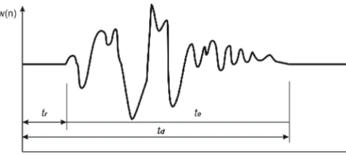
Fig. 1. Example of an impulse response of an echo path.
an estimation of the entire echo path response. The typical echo path delay (td) is formed by a pure delay (tr) and a tail
delay (te) (see Fig. 1). The pure delay is the actual
propagation time taken by the signal from its source to a place where the echo occurs (e.g., hybrid) and backwards. The tail delay, on the other hand, is the response of the hybrid circuit which terminates the four-wire line and performs impedance matching. Not all of the echo path response is relevant to the calculations of an echo canceller. The pure delay element and any portion coming after the tail delay is not relevant and accordingly need not be involved in the adaptation process of the echo canceller. Since an echo canceller’s complexity is related to the number of filter taps it uses, the reduction of the number of these filter taps is important for optimization of filter operation. In order to minimize the echo canceller’s calculations, an estimate of the echo path delay needs to be calculated such that the actual number of required taps may be determined. Therefore, a method determining the du-ration of these portions of the echo path response is necessary to optimize an echo canceller. Methods for determining pure delay estimates from an estimate of the echo path impulse response are described in [1]-[5]. Reference [1] performs a search on the coefficients of the adaptive filter to find the maximum absolute value, corresponding to the peak of the echo path response. According to that technique (illustrated in Fig. 2), assum-ing that the maximum value at coefficient or filter tap wmax,
a value wstart is calculated by subtracting a fixed integer
from wmax. Assuming that the hybrid impulse response lasts
Fig. 2. Graphical view of echo path delay estimation in [1].
Fig. 3. Graphical view of echo path delay estimation in [2].
wstart , then the end of the relevant portion of the impulse
response is wmax + H-1. This provides the boundaries for
the segment te , which is the only portion of the echo path
required for echo cancellation. Once this is established, the adaptive filter echo canceller operates on interval te, and
will only use interval tr as pure delay.
However, a problem with the technique described above is its assumption that wmax lies a fixed integer
amount of samples from the start of the hybrid response. When this assumption is not applicable to a certain system, there is an erroneous echo path calculation, causing the filter to diverge and disrupt the communication. Therefore, it is necessary in implementing this technique that there is a calibration to the type of line characteristics of each application.
Reference [2] describes a two step method that first searches for the maximum absolute value (wmax_1)
con-tained in the first D coefficients of the filter. A second step starts at this position and involves a search for the first ensuing filter coefficient (wmax_2) with an absolute value,
which is K times greater than the first maximum value. The dispersive part of the impulse response is assumed to start a predetermined number of taps before this second tap and to last a predetermined number of taps from this start po-sition. A beginning of the impulse response (wstart) is
calculated as wmax_2 – D. Fig. 3 shows a graphical view
depicting echo path delay estimation using the described technique.
The above described method assumes that the first coefficients of the impulse response have zero mean. However, this assumption is not always true, which may lead to erroneous decisions. For example, the estimated impulse response may contain oscillations with rather long periods, due to filter coefficient estimation using telephone
band speech signals in the presence of background noise from the near end side.
In the method described in [3] the echo location is determined by calculating the echo path location at which there is a high correlation between the signal outgoing to the echo path and the returned echo. The technique uses normalized cross-correlation function for this purpose. The correlation is calculated in a sliding window having the length of the digital adaptive filter. The dispersive part is assumed to start half the filter length before the position of the maximum absolute value of the impulse response estimate. This is not an especially accurate method, be-cause the tap with maximum absolute value does not need to be located in the centre of the echo tail. Moreover, this method breaks down if the impulse response consists of multiple echoes.
Reference [4] describes a method that determines regions of the impulse response where the energy is con-centrated. This is done by summing the absolute values of filter taps within a window with a predefined length and comparing each sum to a fixed threshold. The window slides over the impulse response estimate. The positions exceeding the threshold are considered to belong to echo containing regions. The remaining regions are considered to be delays. This method gives a rather coarse delay measurement. However, no method for choosing a fixed threshold value is presented.
Reference [5] is similar to reference [4] in that it describes a method that determines where in the filter impulse response the energy is concentrated. According to that method, an estimate of the average power in the waveform is computed sample by sample and when a predetermined average power threshold is exceeded a start flag is set. The power calculation is continued until the time when the average power drops below a second threshold indicating that the end of the echo signal has been passed. In order to refine the approximate location of the echo, the method utilizes a computation referred to as centre of echo. This computation is done over the entire range of samples between the first and the second flags. It is assumed that the energy of echo tail is equally distributed about the estimated centre of echo. Then, the radius of echo is computed. It is further utilized to determine the range about the centre of echo which contains the dispersive part of the echo path. However, an assumption that the dispersive region is equally distributed about the estimated centre of echo, which is simply the position of the tap with maximum absolute value, is not true.
Thus, a method and apparatus for accurately determining echo path delay, as well as for accurately determining an appropriate number of taps to utilize for a transversal adaptive filter of an echo canceller is required. It is undesirable for an echo canceller to operate at times when there is no echo. Running an echo canceller under such circumstances merely creates computational
noise as a result of finite word length accuracy in the digital transversal filter. It is therefore desirable to provide a digital echo canceller structure which overcomes these and other problems associated with conventional echo canceller structures.
2.
Dealing With Additive and
Measurement Noise
The above described procedures assumes that the echo path impulse response has been estimated using signals that are rich enough (for instance in their frequency content) to excite all the models of the actual echo path. In several cases, especially if the background noise level from the near end side has been higher than the background noise level from the near end side during a call, the impulse response (IR) estimate will contain errors at frequencies that have been under-represented in the far end signal. Existence of this kind of error components makes the testing procedure less reliable, since the variance of this type of errors is not known. In order to reduce the influence of this type of errors on the impulse response estimate, the impulse response estimate should preferably first be processed to remove (suppress) components that are normally not present in telephone band speech signals.
Echo cancellers are always designed to operate for the limited echo path delay capacity. This creates an additional computational noise as a result of finite word length accuracy. Moreover, when an estimation process is cor-rupted by random variations, it is said to be affected by measurement noise. Since the standard deviation is a meas-ure of spread in a data distribution, these random variations can be characterized by the standard deviation of the measured signal. That is, the larger the standard deviation, the noisier is the measurement. The procedure of reducing or attenuating the noise components of a measured signal is commonly known as filtering. There are many different ways to design filters, but the most common ones have
their roots in simple averaging. Known noise reduction techniques can be classified as follows:
using averaging filter,
using low-pass filter,
by spectral subtraction (Fourier, Wavelet thresholding),
using convolution with smoothing functions.
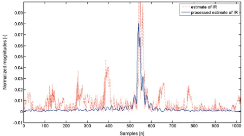
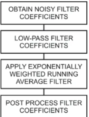
Consider a three stage process of smoothing noisy components. Fig. 4 shows a curve depicting the estimated impulse response and processed estimate of the echo path obtained by a Multi-Delay block Frequency domain (MDF) adaptive filter [6]. The depicted estimate of the echo path impulse response has a lot of noisy components due to the above discussed reasons. The smoothed version of it was obtained in accordance with the procedure show in Fig.5. It is a flowchart illustrating steps performed by an algorithm in order to reduce the influence of measurement errors. The first operation is low-pass filtering. This is done by transforming the filter coefficients using the Fast Fourier Transform (FFT) into the frequency domain. The frequency bins, which lay under the predefined cut-off fre-quency (e.g., Fcut = 200 kHz) are removed from the
spectrum. Then, the inverse FFT (IFFT) is applied to transform the filter coefficients back into the time domain. The second step uses the exponentially weighted moving average filter. This operation is performed in accordance with the following expression
k k k w w w 1 1 , (1) 1 1 1 WIN WIN , (2)
1 1 1 1 WIN (3)where wk are the low-pass filtered coefficients, k = 1, 2, …,
L (L is the adaptive filter length); WIN1 is a moving
window of k values (e.g., 8 samples or 1 ms for 8 kHz sampling rate) that are used to calculate the average of the data sequence; αis the filter constant (forgetting factor).
Fig. 5. A flow chart illustrating a smoothing procedure.
Its value dictates the degree of filtering, i.e. how strong the filtering action will be. Since k≥ 0, this means that 0 ≤α < 1. When a large number of points are being considered, α → 1, and wk→wk1. This means that the
degree of filtering is so big that the measurement does not play a part in the calculation of the average. On the other extreme, if k→0, then wk→ wk which means that virtually
no filtering is being performed.
After the previous step has completed, the averaged filter coefficient should be post processed in the following manner
1 1 , 1 , 1 0 , 1 1 2 2 2 0 2 2 L k WIN when w WIN WIN k when w WIN h k WIN k u u k u u k (4)where WIN2 is the second moving window of k values
(e.g., 8). The reason for doing this operation is to facilitate the searching scheme for dispersive regions. The following section describes a proposed method for echo canceller which determines the dispersive regions from the processed estimate of the echo path impulse response.
3.
Determining Dispersive Regions
That is, the overall echo canceller structure looks like a conventional echo canceller having a very large tapped delay element. But, only certain groups of taps are actually turned on at any given time, after the dispersive regions have been defined. The present algorithm examines the impulse response of the line (which corresponds to tap weights for a transversal filter) and allocates taps according to where an echo is actually occurring on the line. Consequently, an echo canceller includes a long transversal filter incorporated with the control element used to estimate the delays and widths of the dispersive regions. The transversal adaptive filter has length large enough so that the whole echo path impulse response (td) can be
estimated. Delay values are then estimated from the filter coefficients. When all delays are known, the number of filter taps can be greatly reduced.
When the connection starts (t0), the adaptive filter is
activated to estimate the echo path. Note, some predetermined conditions are employed to decide when the transfer of filter coefficients to the control network should occur, and these preconditions are the following. First, the approximate settling time (1 second + td + t0) for the
adaptive filter is calculated. Afterwards, this value is transferred into the counter register of the control network. This condition assures the adaptive filter will have enough time for adaptation, but no guarantee of accuracy. When double-talk situation is detected, the counter is frozen since the weight adjustment process has been prohibited. After the settling time has expired, the second condition is tested. One should still be aware that no double-talk is present, since near-end speech will affect the test result. Thus, when the first condition is satisfied and there is no near-end speech in the line, the short time powers of e(n) and y(n)
n 1
1
e2 n, R Re e (5)
n 1
1
y2 n, R Ry y (6)are calculated and then their ratio is compared to a small constant value χ. A χ of 0.01 corresponds to a 20 dB loss of echo power. Weighting factor, ρ, is a constant between 0 and 1, for example 127/128. Furthermore, the power may also be estimated by summing the squares of, for example, the last 128 samples of e(n) and y(n), but equations above require a less complex implementation. Alternatively, a quantity called the Echo Return Loss Enhancement (ERLE), represented by the following equation
], [ , log 10 ) ( 1 2 1 2 10 dB e y n ERLE n N n i i n N n i i
(7)may be used for testing the second condition. When all the conditions are satisfied, the control network will copy the filter weights, process them and perform the search for the echo delays. The method for locating the dispersive regions of the function h(k) is as follows:
a) find the maximum (hmax) value of the h(k), store
its position, as hmax_position;
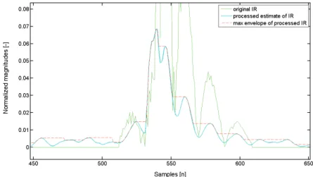
b) calculate the maximum envelope (hmax_envelope, see
Fig. 6) using algorithm shown in Fig. 7;
c) search for the 1st interval on the left from the
hmax_position, where hmax_envelope is constant;
d) store the value of hmax_envelope into variable
hmax_1_right;
e) search for the 2nd interval on the left from the
hmax_position, where hmax_envelope is constant
f) store the value of hmax_envelope into variable
hmax_2_right;
g) find local minimum of the function h(k) within the 1st interval and store it, as h
min_1_right;
h) find local minimum of the function h(k) within the 2nd interval and store it, as h
min_2_right;
Fig. 6. A graph illustrating a smoothing procedure.
else h h C right right , 0 0 , 1 1 min_1_ min_2_ , (8)j) calculate the 2nd condition (C2) using equation
else h h h h C right right right right , 0 % 40 % 100 , max , 1 2 max_1_ max_2_ _ 2 max_ _ 1 max_ , (9) k) calculate the 3rd condition (C3) using equation
else h h C right right , 0 0 , 1 3 max_1_ max_2_ , (10)l) check these three conditions in accordance with the coding scheme illustrated in Fig.8;
m) define, whether the 1st region attends to the
dispersive part of the echo impulse response (IR); n) copy parameters from the 2nd interval into the 1st
interval;
o) search for a new 2nd interval on the left from the
1st interval, where h
max_envelope is constant;
p) perform steps 6-15 again, till the end of the left-hand region of the function h(k);
q) repeat steps 3-4 again, but for the samples, which lay on the right side from the hmax.
Note, that, when the end of the dispersive region is found, the steps n) and o) are excluded. Also note, that in order to simplify the search operation, only intervals (where hmax_envelope has constant values) with the length
bigger than, e.g., 8 samples may be considered. After all the steps have passed, the width of the first dispersive region (wwidth) can be determined using the following
equation formulas start end width w w w , (11) right start h w min_1_ , (12)
Fig. 7. An engine for searching max envelope of the post-processed estimate of echo path.
Fig. 8. A transition diagram for testing conditions C1, C2, C3.
right start h w min_1_ , (12) left end h w min_1_ . (13)
Fig. 9. A simplified structure of a new frequency domain filter.
If the case with multiple dispersive parts is considered, the values of the function h(k), which belong to the determined dispersive region have to be turned to zero.
Afterwards, the whole searching operation may be repeated. Nevertheless, the time delay estimate of the entire echo signal should be preferably calculated in accordance with the following relationship
1 0 2 1 0 2 L k k L k k s n w n w k T n Delay (14)where Ts=1/Fs, Fs is a sampling rate of speech signal (e.g.,
8 kHz); wk is a particular adaptive filter weight. For the
purpose of the subsequent section define a binary vector (BIN) of length L. Its elements are formed in the following manner
elsewhere. , 0 IR, the of part dispersive the inside lays if , 1 w n n BIN k k (15)After the dispersive regions are determined, the control circuit sets the adaptive filter. The active weight values are remained turned on. To improve the accuracy of the adaptive filter, an echo estimate is calculated only using certain subfilter blocks, which are considered to cover the dispersive part of the echo path impulse response (IR).
4.
Proposed Echo Cancelling
Algorithm
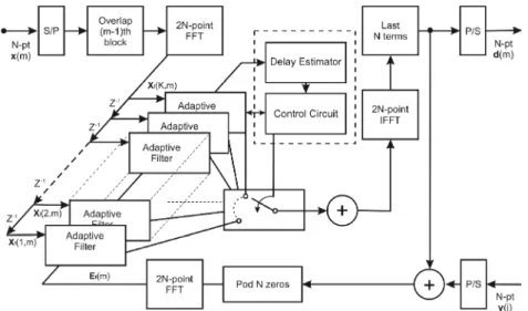
A simplified block diagram of the proposed adaptive filter is shown in Fig. 9. Its structure consists of an echo estimator, K short length (N) subfilter blocks, an output multiplexer, and a control circuit. The delay estimator is a primary whole length (L = KN) MDF or any other
frequency domain filter [7] incorporated with the control circuit used to estimate the delays and widths of the reduced dispersive regions. Note, that the value of L should be large enough so that the whole echo path impulse response can be covered. In some commercial echo canceller structures this value may be up to 4096 samples, which corresponds to the delays up to 512 ms. Echo path delay can then be determined from the estimated echo path impulse response. When all the delay values are known and the binary vector (BIN) is formed, the number of operations required for calculation of the echo signal can be greatly reduced. The output multiplexer, which is controlled by the control circuit, selects which coefficients within the adaptive filter need to be updated or not. Note that the whole length filter still may function as a weight updater. Both types of structures, the full-length and the short one, are operating exclusively. The control circuit can compare the errors from these filters to determine which one is more suitable for that instant of time to estimate echo path. In order to track the time variance of the echo path, the control circuit has to check for the location of the maximum weight value of the dispersive region to adjust the elements in the vector BIN(n) after a specified settling time (tcheck). In this way, each subfilter block can track its
own dispersive region more efficiently and accurately. The improvement in accuracy is a direct result of the fewer weights needed since the misadjustment is proportional to the number of weights [8].
The first step of the MDF algorithm is to convert the most recent overlapped input samples to the frequency domain as follows
. , ... , , , 1 , ... , 1 , 1 , 1 1 0 1 1 0 T N N f x m x m x m x m m x m x FFT diag m K X (16)The input vectors incoming to each of the subfilter blocks can be obtained via the frame index shifting without invoking any computation as follows:
k,m
f
k1,m1
, k1,...,K1.f X
X (17)
The described approach suggests that only one FFT is needed per frame iteration in order to transform the input vector into the frequency domain. It implies a significant computation saving. The output and the error frequency-domain vectors can be expressed and calculated as
last termsof
,
, , 1 1
K k f f k m k m FFT N m X W d (18)
0,0,...,0,
, terms zeros N N f m FFT y m dm E (19)
terms zeros , , 0 , ... , 0 , 0 , N N f k m FFT wk m W (20)where Wf(k,m) is the kth frequency coefficient vector and
d(m) is the desired vector. The IPMDF time coefficient update equations to minimize the Mean Square Error (MSE) are the following
k m
FFT
f
k m
SMDF
m
f
m
t X E φ , firsthalf of 1 , 1 (21)
m S
m 1
1
k,m
k,m
, SMDF MDF Xf Xf (22)
k,m 1
w
k,m
L k Gt
k,m
φt k,m
w , (23)
k m
diag
gkN
m gkN
m gkN N
m
t , , 1 ,..., 1 G , (24)
1 0 2 1 2 1 L j j l kN l kN m w m w L g (25)where k = 1, 2, …, K, l = 1, 2, …, L and μk is the block
step-size control parameter, 0 << λ < 1 is the forgetting factor. Further, we describe how the binary vector BIN
may be incorporated into the IPMDF algorithm. Define the LxL diagonal selection matrix B(m)
m diag
bkN1
m,...,bkNN
m
,k 0,...,K1 kB
(26)
and its elements are defined as follows
. 0 , 0 , 1 , ... , 0 , 1 , 1 l l l BIN LI L l BIN LI m b (27)The time-domain subfilter-selection routine is done by multiplying this matrix with the corresponding weights in every kth subfilter, as shown below
k,m 1
w
k,m
L k B
k,m
Gt k,m
φt k,m
.w (28)
Interchanging between the full-length IPMDF and the reduced length IPMDF is done every tcheck milliseconds
(e.g., 16 ms). If the performance of the algorithm decreases, the control circuit originates a new search for the active regions of the echo path impulse response.
5.
Results of Experiments
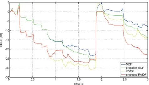
To evaluate the performance of the proposed algorithm, we implemented it as well as conventional adaptive filters in MATLAB environment. Both the conventional and the proposed adaptive filter structures are used to cancel simulated echo signal. The simulated echo signals are generated by using the models of the echo path impulse response specified in the corresponding ITU-T Recommendation [9].
For the simulation, the following main parameters are used: Fs = 8000 Hz, L = 1024, K = 8 and ERL = -6 dB. The
performance of each algorithm is evaluated by using the normalized Echo Return Loss Enhancement (ERLE) para-meter, which is used in real-life environment to evaluate the performance of an echo canceller. ERLE for each algorithm was calculated according the (7). In each experi-ment the delay of the echo path changes after the pre-defined period of time. The example ERLE curves for both the conventional and the new structure are shown in Fig. 10.
As it can be seen from the figure the proposed scheme for the MDF/IPMDF performs better over the conventional fully updated frequency domain algorithms. In comparison to conventional algorithms for echo cancelling the computational complexity, the convergence speed and the degree of estimation accuracy in the adaptation process are improved in proposed method.
It was an object of this paper to provide an improved echo canceller circuit which reduces computational noise when there is no echo to cancel. It is another object of the present research to provide an improved echo canceller structure which rapidly adapts to intermediate echoes. A method of allocating filter taps in an adaptive filter for a transmission line includes the steps of storing samples of the transmission line’s impulse response in a memory; examining the stored samples to find ranges of samples of the impulse response having echo energy; and allocating a variable number of filter taps of the adaptive filter only to taps within the ranges of samples having echo energy. A delay estimator detects ranges of samples within the impulse response having echo energy. An adaptive filter includes a plurality of weights. A control circuit activates and deactivates variable numbers of taps in response to the delay estimator so that only taps within the ranges of samples are activated within the adaptive filter. The output multiplexer operating under the control circuit selects the estimated echo outputs from a plurality of the subfilter blocks in order to calculate an echo signal, which is then subtracted from the incoming signal.
Fig. 10. Comparison in terms of misalignment and ERLE parameters.
6.
Conclusion
This paper addresses the problem of echo assessment, echo path’s delay estimation, design of robust, low computational complexity and fast converging adaptive filters for echo cancellation. Both conventional and hands-free telephone sets, occupy a prominent position in com-munications. One of the major problems over a telephone system is echo. The adaptive filtering algorithms and the detector of the dispersive regions presented in this paper successfully suggest an approved solution for existing echo problem in the telecommunications environment.
During our future work we intend to upgrade the above described algorithms. The proposed delay estimator and the control circuit may be used in conjunction with an adjustable delay block in order to compensate a flat delay presented in the echo path.
Acknowledgements
Thanks to the grant SGS No.OHK3-108/10 of the Czech Technical University and the research program MSM 6840770014 of the Ministry of Education, Youth and Sports of Czech Republic for funding.
References
[1] MONTAGNA, R., NEBBIA, L. Method of and Device for the Digital Cancellation of the Echo Generated in Connections with
Time-Varying Characteristics. U.S. Patent No. 4,736,414, 1988.
[2] MALKI, K. E. Echo Path Delay Estimation. U.S. Patent No. 5,920,548, 1999.
[3] VAHATALO, A., MAKINEN, J. Method Determining the
Location of Echo in an Echo Canceller. U.S. Patent No. 5,737,410,
1998.
[4] YIP, P. C-W., ETTER, D. M. An adaptive multiple echo canceller for slowly time-varying echo paths. IEEE Transactions on
Communications, 1990, vol. 38, no. 10, p. 1693 - 1698.
[5] MARTINEZ, A. A. Echo Canceller with Dynamically Positioned
Adaptive Filter Taps. U.S. Patent No. 4,823,382, 1989.
[6] SOO, J. S., PANG, K. K. Multidelay block frequency domain adaptive filter. IEEE Transactions on Acoustics, Speech and Signal Processing, 1990, vol. 38, no. 2, p. 373 - 376.
[7] KHONG, A. W. H., BENESTY, J., NAYLOR, P. A. An improved proportionate multi-delay block adaptive filter for packet-switched network echo cancellation. In Proceedings of the 13th European
Signal Processing Conference EUSIPCO '05. Antalya (Turkey),
2005.
[8] WAGNER, K., M. DOROSLOVACKI, M. Proportionate-type normalized least mean square algorithms with gain allocation motivated by mean-square-error minimization for white input.
IEEE Transactions on Signal Processing, 2011, vol. 59, no. 5,
p. 2410 - 2415.
[9] ITU-T Recommendation G.168, Digital network echo cancellers, Geneva (Switzerland): ITU, 2009.
![Fig. 2. Graphical view of echo path delay estimation in [1].](https://thumb-us.123doks.com/thumbv2/123dok_us/863943.2610279/2.892.83.453.108.488/fig-graphical-view-echo-path-delay-estimation.webp)