Online Full Text

Abstract: Profit and risk are perhaps the most important criteria in investment analysis. This paper aims to solve the question of how to measure the risk-return relationship for investments in emerging economies. Financial theory and a lean statistical technique are employed to perform such analysis. Stock market indexes’ behavior is observed and analyzed, while the risk and return of emerging economies are measured by estimating the parameters of the Capital Asset Pricing Model (CAPM) for the returns of 31 stock market indexes. Betas and Jensen’s alphas are estimated from the CAPM, and Sharpe and Treynor ratios are calculated from historical records of return and volatility. Finally, principal component analysis is used to build a performance benchmark of stock markets in emerging countries.

Index terms: Emerging countries, Jensen’s Alpha, performance benchmark, Sharpe Ratio, Treynor Ratio.

I. INTRODUCTION

One of the most important criteria in investing is the risk-vs.-return performance of the investment alternatives. However, this information is not always available to potential investors, especially in emerging economies.

This paper aims to build a performance benchmark for emerging markets. This is done in two steps. First, a qualitative analysis is conducted for a sample of emerging countries, based on the behavior of the following financial variables from January 2006 to November 2011:

1. Stock market indexes

2. Intermediation margin of credit default swaps (CDS)

3. Risk aversion index (VIX)

Secondly, Betas and Jensen’s alphas are estimated by applying a least squares dummy variable method (LSDV).

Manuscript received March 18, 2012, and revised April 3, 2012. This paper is based on the MSc dissertation of Juan Sebastián Lemus Esquivel completed at Universidad de los Andes in Bogotá, Colombia during the second semester of 2011.

Juan Sebastián Lemus Esquivel holds a Bachelor of Science degree with honors in Industrial Engineering and a Master of Science degree in Operations Research, Statistics, and Finance from the School of Engineering at Universidad de los Andes. He currently works as a financial analyst in the Financial Stability Department at Banco de la República (Colombia’s central bank). Phone: +57 (1) 343 0994. Email: [email protected].

Laura Juliana Oyuela Eslava holds a Bachelor of Science degree with honors in Industrial Engineering from the School of Engineering at Universidad de los Andes. She is currently pursuing a Master of Science degree in Operations Research, Statistics, and Finance at Universidad de los Andes. In addition, she works as a graduate teaching assistant in financial risk management. Phone: +57 (1) 339 4949, ext. 1823. E-mail: [email protected].

Professor Julio E. Villarreal N. is the director of the Economics and Finance academic area within the Department of Industrial Engineering at the School of Engineering at Universidad de los Andes. Phone: +57 (1) 339 4949, ext. 2883. E-mail: [email protected].

This model (linear regression) is an extension of the Capital Asset Pricing Model, in which intercepts (alphas) and slopes (Betas) differ according to the countries. Thereafter, ex-post performance measurements such as Sharpe and Treynor ratios are calculated based on the previously mentioned parameter estimations.

Finally, principal component analysis is applied to the Jensen’s Alpha and the Sharpe and Treynor ratios estimates to build a performance index to rank the evaluated emerging economies. Based on these estimates and the analysis conducted, the emerging economies’ performances are evaluated. We conclude that emerging markets’ stock indexes do not beat the market portfolio proxy and that investing in emerging economies is not efficient.

II. EMERGING MARKETS

Public market information on 31 countries classified as emerging economies is taken as the input to build a performance index benchmark.

A market must fulfill four conditions to be labeled as an emerging market (Mody, 2004):

1. Its stock market presents high volatility and, therefore, an investment is perceived as significantly risky by international investors.

2. It has the potential to develop mature financial and political institutions, allowing it to become a player in the world economy in the mid-term.

3. Its stock market indexes offer high returns; however, their historical and expected returns are lower than those of observed for developed economies’ stock market indexes.

4. It has lower levels of foreign investment than those in developed countries.

The 31 markets we chose to study were classified as “emergent” by Dow Jones (2010) and Standard and Poor’s (2010). The chosen countries and their stock exchanges (in parentheses) are:

--Africa: Morocco (Casablanca Stock Exchange), Mauritius (Stock Exchange of Mauritius), South Africa (Johannesburg Stock Exchange)

--Latin America: Argentina (Buenos Aires Stock Exchange), Brazil (Brazilian Securities, Commodities and Futures Exchange), Chile (Santiago Stock Exchange), Colombia (Colombia Stock Exchange), Mexico (Mexican Stock Exchange), Peru (Lima Stock Exchange)

--Asia: Bahrain (Bahrain Stock Exchange), China (Shanghai Stock Exchange), the Philippines (Philippine Stock Exchange), India (Bombay Stock Exchange), Indonesia (Jakarta Stock Exchange), Kuwait (Kuwait Stock Exchange), Malaysia (Bursa Malaysia), Pakistan (Karachi Stock Exchange), Qatar (Doha Stock Exchange), Sri Lanka Juan Sebastián Lemus Esquivel, Laura Juliana Oyuela Eslava, Julio E. Villarreal Navarro

(Colombo Stock Exchange), Thailand (Stock Exchange of Thailand)

--Europe: Bulgaria (Bulgarian Stock Exchange), the Czech Republic (Prague Stock Exchange), Estonia (Tallinn Stock Exchange), Slovakia (Bratislava Stock Exchange), Hungary (Budapest Stock Exchange), Poland (Warsaw Stock Exchange), Romania (Bucharest Stock Exchange), Russia (Moscow Interbank Currency Exchange), Turkey (Istanbul Stock Exchange).

III. QUALITATIVE ANALYSIS

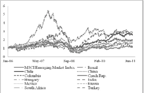
To analyze the performance and behavior of the selected emerging economies over the defined time window (January 2006 to November 2011), a record is kept of these economies’ market indexes and of the intermediation margin of the credit default swaps and the VIX.1 The last two indexes allow us to infer about international investors’ aversion to market and default risk exposure. Fig. 1 shows the behavior of these variables.

Fig. 1. Returns of the MXEF index and some emerging market indexes from January 2006 to June 2011. Source: Bloomberg.

Fig. 2. Behavior of risk aversion index VIX and intermediation spread of CDS for emerging markets from January 2006 to June 2011. Source: Bloomberg. 

The following conclusions can be made from Fig. 1 and Fig. 2, based on the most relevant facts that appeared on the Financial Stability Reports published during the analyzed time window by the central bank of Colombia (Banco de la

       1

   Chicago Board Options Exchange SPX Volatility Index.

República):

1. Stock indexes showed weak performance and the VIX and Intermediation CDS margins presented high values during two time periods: from the second half of 2007 to the first trimester of 2009 and from February 2011 to November 2011. 2. The subprime mortgage crisis which lead to the

2008 global financial crisis took place during the first period, while the natural disaster in Japan and the debt market crisis of the P.I.G.S. countries (Portugal, Italy, Greece and Spain) occurred during the second period.

3. The previously mentioned situations had a generalized, negative impact on the analyzed emerging economies, diminishing market performance and the expectations of economic growth.

4. Emerging markets tend to react homogenously in response to performance expectations of great powers’ economies. However, the global and unexpected economic events impacted developed economies first and emerging countries later. For example, Latin American and African economies received the negative impact of events (such as the 2008 subprime mortgage crisis and the 2011 disaster in Japan) later than European and Asian economies, as the latter economies have more direct relationship with great powers (U.S., Germany, Japan, U.K., France, etc.).

5. Emerging economies’ stock markets react negatively to crisis and positively to high growth expectations of developed economies.

IV. QUANTITATIVE ANALYSIS

To build the performance benchmark, three indexes are examined:

--Jensen's Alpha: Aims to evaluate portfolio performance (Jensen, 1967), which is defined as:

1. The capability of a portfolio manager to increase a portfolio’s return through a “successful forecast of future expected prices of the portfolio assets” (Jensen, pp.1).

2. The capability of a portfolio manager to minimize portfolio holders’ exposure to systematic risk. Based upon the previous definition, the Jensen's Alpha of asset i ( ) is directly estimated as the intercept of the CAPM

E R rf α β E R r ε

where

E R is the expected return of asset i in period t rf is the spot value of a risk-free asset in period t

β is a sensitivity measure and quantifies systematic risk of asset i

their risk exposure. Called ex-post since it is based on historical information of its input variables.

Sharpe (1994) defines it as

S ≡ D

σ where

is the mean of observed excess return of asset i

is the estimated standard deviation of observed return excess for asset i

--Treynor Ratio: Measures efficiency based on historical volatility (Treynor, 1965). Records of historical price volatility are good references for the evaluation of future performance. Mathematically, the ratio is defined as:

T ≡r r

β where

r is the expected return of a fund i r is the risk-free rate

β is the systematic risk of a fund i

According to Sharpe (1966), even if the Treynor index produces a portfolio performance ranking similar to that of the Sharpe Ratio, the first one captures the variability caused by lack of diversification. However, Sharpe argues that Treynor Ratio is a reasonable measure to predict future performance. Both Sharpe and Treynor ratios can be calculated based on the estimates derived from CAPM (Betas, the risk-free rate, and market risk premium).

A. Data collection and processing

The input information required to feed the LSDV regression is organized in panel data. The spot prices of the 31 emerging-economy stock market indexes are analyzed across 67 months (from January 2006 to July 2011). Based on the recommendations of Morningstar (2011), a longer time window cannot be considered, given that, in general, no longer-term information is available for emerging markets. Also, estimation via the ordinary least squares method (OLS) has proven that emerging economies’ Betas are unsteady over time.

The selected proxy for the risk-free rate was the monthly returns for four-week maturity treasury bills. The index used as a proxy for the market portfolio is the Morgan Stanley Capital International Emerging Markets Capital Index (MXEF), as this index measures the joint performance of emerging markets. Because the start and end dates were not homogeneous for all countries, only the last price P of every month was taken into account to calculate the monthly return of all the indexes: Let T be the set of all the months in the defined time window, and let J be the set of the 31 emerging markets. The return for index j in month t is calculated as follows

E R ln P

P 1 ∀ j ∈ J, ∀ t ∈ T

B. Parameter estimation by ordinary least squares To estimate the Jensen’s Alpha and the Betas of the emerging economies, the following LSDV formulation is proposed:

E R rf α α D α D ⋯ α D

λ D λ D ⋯ λ D

γ D X γ D X ⋯

γ D X u

1,2,3, … , 1,2,3, … , 1,2,3, … ,

where

is the individuals’ cross-section units (countries) is the set of time periods (months)

E R rf is the dependent variable, the excess of return of economy i over the return of the risk-free asset in time period t.

D is a dummy variable, introduced to estimate a different intercept and slope for each country,

D 1 0

if i j if i j

X E R rf is the independent variable, the

excess of return of the market portfolio over the return of the risk-free asset in time period t.

D is a dummy variable introduced to control for time effects,

D 1₀ if the observation is made in k _otherwise , k 2006, 2007, 2008, 2009, 2010, 2011

According to Greene (2008) and Cameron and Trivedi (2009), for this model to be reliable, it has to follow the following assumptions:

--The functional form of the model is linear. --The matrix of the independent variables has to have full rank.

--Residuals (u ) fit to a white-noise process, which means that:

E u 0, E u σ , Cov u , u 0

The next step was to derive the estimation of the parameters via OLS. Afterwards, the model was evaluated to verify that it fulfilled the assumptions. If the model did satisfy such assumptions, it could be labeled as valid; if it did not, anomalies were corrected.

C. Tests

Some statistical tests were carried out to verify that the model satisfied the previously mentioned assumptions. When an anomaly was identified for some individual (country), a correction was performed. The tests and corrections were performed in a sequential manner as follows.

1) Ramsey test

This test verified that the functional form of the model was accurate or, in other words, correctly specified. The results of the test suggested that the LSDV model specification should be revised or redefined.2 However, the

       2

 Sufficient statistical evidence showed that the LSDV model is

CAPM was the model that best fit our research objectives, since it allowed the identification and estimation of a linear relationship between risk and return, and, financial theory is to a great extent based on this model. Therefore, we kept this model, taking into account that the estimators may be biased.

2) Conditions for the error

According to Gujarati (2003) and Griffiths et al. (1993), the observed error of the model, (u must fit a white-noise process, in order for the OLS estimators to be considered valid.

Using the Q statistic of the Ljung-Box test, it was possible to assess whether the idiosyncratic errors of each cross-section unit satisfied the conditions of homoscedasticity and absence of serial correlation. We found that there was a low probability of making a mistake when rejecting the null hypothesis of this test for 16 cross-section units. Therefore, heteroscedasticity and correlation problems for these units were suspected.

3) Correction for heteroscedasticity

According to Long and Erwin (1998), the heteroscedasticity-consistent covariance matrix (HCCM) must be used when suspecting heteroscedasticity in an OLS model. The HC1, HC2, and HC3 corrections are applied to the panel data. The HC3 correction was selected as optimal, based on the fact that it has been proven to show the best performance when correcting extreme heteroscedasticity cases (Long & Erwin, 1998). However, the estimations from the corrected model did not differ significantly from those obtained by the LSDV regression. This occurs since the HCCM corrections assume no correlation. In particular, only Slovakia’s idiosyncratic error term fitted to a white noise after applying the HC3 correction. The remaining 15 cross-sections3 were confirmed to present serial correlation, based on the observed behavior of the estimated autocorrelation functions (ACF) of their estimated errors.

4) Correction for residuals that do not fit to a white-noise process

Residuals must fit to a white noise process (random variables with mean zero, finite variance and uncorrelated). If this is not the case, the variance can be stabilized using the method proposed by Guerrero (2003), which determines a variable transformation. After this methodology was applied, we found that no transformations were needed for the estimated residuals of the 15 “problematic” countries.

Afterwards, the Box-Jenkins iterative methodology was applied to find the autoregressive moving average (ARMA) model that correctly describes the behavior of OLS-estimated residuals for each cross-section. When the parameters of the ARMA (P,Q) model for each error term were estimated, the OLS model was re-estimated, taking this new information as an input.

To incorporate the observed errors that follow an ARMA (P,Q) process in the estimation of the OLS model, four estimation techniques were applied:

--Two-step full transformation method

and fourth power of the predicted dependent variable are equivalent to zero—was rejected.

3

 The 15 “problematic” countries are Bahrain, Chile, Estonia, Hungary,

Jordan, Kuwait, Malaysia, Oman, Pakistan, Peru, Poland, Qatar, the

Czech Republic, Romania, and Sri Lanka.

--Iterated Yule-Walker method --Maximum likelihood --Unconditional Least Squares

No significant differences were observed when comparing these estimations’ outputs. To choose the best-fit model, Aikaike information criterion (AIC), Bayesian Schwarz criterion (BSC), and the statistical significance of parameters were taken into consideration. Consequently, the technique with the best overall performance was selected.

D. Final model and estimations

Based on the corrected and final estimated model for each cross-section, the estimations of Jensen’s alphas and Betas were derived. Consequently, it was possible to calculate the Sharpe and Treynor ratios. These estimates are shown In Table 1.

TABLE 1.JENSEN'S ALPHAS, BETAS AND SHARPE AND

TREYNOR RATIOS FOR THE ANALYZED EMERGING

ECONOMIES

Country Jensen's Alpha Beta

Sharpe Ratio

Treynor Ratio Argentina 0.014 1.346 -0.484 -0.010

Bahrain -0.023 0.270 -2.380 -0.101 Brazil 0.000 1.599 -0.221 -0.007 Bulgaria 0.010 0.767 -0.742 -0.035 Chile 0.022 0.675 -0.255 -0.008 China 0.000 1.146 -0.120 -0.003 Colombia 0.014 1.532 -0.401 -0.007 Czech Rep. 0.000 1.621 -0.591 -0.011 Estonia 0.023 1.234 -0.459 -0.012 Hungary 0.007 1.804 -0.508 -0.010 India -0.018 0.484 -0.320 -0.019 Indonesia -0.017 0.653 0.045 0.002 Jordan -0.031 0.499 -1.750 -0.060 Kuwait 0.000 0.523 -1.492 -0.053 Malaysia 0.017 0.704 -0.341 -0.008 Mauritius 0.000 0.657 -0.157 -0.005 Mexico 0.000 0.436 -0.446 -0.024 Oman 0.000 0.633 -0.890 -0.027 Pakistan 0.000 0.510 -0.789 -0.043 Peru 0.015 0.727 0.146 -0.007 Philippines 0.018 1.322 -0.177 -0.003 Poland 0 1.589 -0.427 -0.008 Qatar -0.016 1.457 -0.751 -0.015 Romania 0.000 1.947 -0.626 -0.013 Russia 0.015 1.365 -0.380 -0.009 Slovakia 0.000 1.276 -1.215 -0.019 South Africa 0.014 1.078 -0.509 -0.012 Sri Lanka 0.033 0.592 -0.078 -0.003 Thailand 0.000 1.600 -0.331 -0.005 Turkey 0.023 1.421 -0.463 -0.012

V. PERFORMANCE ANALYSIS IN EMERGING ECONOMY

STOCK MARKETS

guarantees dimensionality reduction.

Principal component analysis is applied to the final performance measures estimates. As a result:

--For the Jensen’s Alpha and Treynor Ratio, there is a high variability between individuals.

--The Sharpe and Treynor ratios present asymmetry and kurtosis values different from those of the standard normal probability distribution. Nonetheless, no variable transformations are applied, since principal component analysis does not require that variables fit any probability distribution. Moreover, transformed variables would lack financial interpretation.

--Correlation between the Jensen’s Alpha and the other two indexes is close to 0.5, and in both cases statistically different from zero.

--Principal component analysis reduces the dimensionality of the problem, explaining most of the variability of the data. The first component explains roughly 80 percent of the variability.

--Consequently, the first component is chosen as the performance measure used to rank the emerging countries. This component is defined as follows:

ID w JA w SR w TR

where

is the subindex for every country

is the weight of variable j in the index, j=1,2,3 is the estimated Jensen's alpha for country i

is the estimated Sharpe Ratio for country i is the estimated Treynor Ratio for country i

--PCA results render that component weights w , w and w are 0.490549, 0.616579, and 0.349747, respectively.

Fig. 3 presents a “biplot,” which is a coordinate system that represents the individuals (countries) and the variables (first and second components) as Cartesian coordinates. The variables are represented as vectors (projections) with respect to the origin, and individuals are presented as points on the map. Sharpe and Treynor ratios are represented in the first quadrant, while the coordinates for the Jensen’s alphas are located in the fourth quadrant. This graphic representation shows that the correlation between the Alpha and the ratios is not significantly strong.

In addition, from the “biplot” is possible to infer the following:

--Peru has the highest Sharpe and Treynor ratios estimates; however, its Jensen’s Alpha estimate is not significantly high.

--Sri Lanka has the highest Jensen’s alpha estimate, with relatively high Sharpe and Treynor ratios as well.

--Turkey and Estonia have high Jensen’s-alpha estimates and average Sharpe and Treynor ratios estimates.

--Qatar and India have low Jensen’s Alpha estimates; however, India has higher Sharpe and Treynor Ratio value than Qatar.

--Jordan, Bahrain, and Kuwait have the lowest values for the three performance indexes.

--China, Mauritius, Brazil, and Thailand have average Jensen’s Alpha estimates; however, they have high Sharpe and Treynor ratios values.

--The Philippines, Chile, Malaysia, Russia, Argentina, and South Africa have the highest Sharpe and

Treynor ratios estimates.

Based on these results, we conclude that the higher the value of the first component, the better the country’s performance.

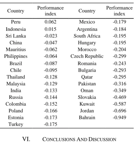
Using the first component, the analyzed countries are ranked as shown in Table 2. A higher ranking means the country had a better performance during the analyzed time period.

Fig. 3. Representation of the individuals (countries) and the first two components in a coordinate system

TABLE 2.PERFORMANCE RANKING FOR EMERGING

COUNTRIES

Country Performance

index Country

Performance index

Peru 0.062 Mexico -0.179

Indonesia 0.015 Argentina -0.184 Sri Lanka -0.023 South Africa -0.195 China -0.047 Hungary -0.195 Mauritius -0.062 Morocco -0.204 Philippines -0.064 Czech Republic -0.299 Brazil -0.087 Romania -0.243 Chile -0.095 Bulgaria -0.293 Thailand -0.128 Qatar -0.295 Malaysia -0.129 Pakistan -0.316

India -0.133 Oman -0.349

Russia -0.144 Slovakia -0.469 Colombia -0.152 Kuwait -0.587 Poland -0.166 Jordan -0.696 Estonia -0.173 Bahrain -0.949

Turkey -0.175

VI. CONCLUSIONS AND DISCUSSION

1. In 2008 and 2011, emerging economies’ stock markets performed poorly and gave a higher perception of risk than the perceived risk for great powers.

2. Poorer performance and an increase in perception of risk are consequences of global economic crisis, such as the 2008 subprime mortgage crisis, the 2011 natural disaster in Japan, and the P.I.G.S. countries’ debt market crisis.

3. Emerging markets were shown to be highly sensitive to economic crises in developed countries. However, the impact they experience comes late: Months can pass before negative effects are evidenced in emerging markets.

4. The most relevant economic events that occurred from January 2006 to November 2011 did not have homogeneous effects on emerging markets. For example, the subprime mortgage crisis led to a global financial crisis in 2008 that affected debt markets worldwide, while Japan’s natural disaster and the crisis of some European debt markets had an impact in Asia and Europe, respectively. It is expected that in the short term, the European sovereign debt crisis will have a moderate impact in emerging countries.

Thirty-one economies were studied, all of which were characterized as emerging by credit-ranking agencies and whose market information was available. Three ex-post performance measurements—Jensen’s Alpha, Sharpe Ratio, and Treynor Ratio—were calculated based on the information of the respective stock indexes of each economy. These measurements were estimated through a lean methodology, the first step of which was estimation by a LSDV method. Then, to obtain reliable estimates of the Beta and the Jensen’s Alpha for every individual, some corrections were made based on econometric and time series analysis in order to satisfy OLS assumptions. The estimates carried out in this study are dependent upon the input information. It is possible that different information used to estimate the key parameters (Betas, Jensen’s Alpha), would provide different results.

We succeeded at integrating the information of the three performance measurements analyzed by means of principal component analysis. Results show that the first component accounts for 80 percent of the variability in the data. This component is a performance index for emerging markets that weights Jensen’s alpha and Sharpe and Treynor ratios. We built a relative notion of performance, avoiding individual analysis and interpretation of the three performance measurements.

The results of the Principal Components Analysis allowed us to obtain a ranking of the different emerging countries under study. The ranking was done based on their stock market performance from January 2006 to July 2011. The estimates of the Jensen’s alphas for the stock market indexes were very close to zero, which supports the argument that stock markets follow the weak form of market efficiency proposed by Fama (1965). In this manner, the prices of

stock indexes incorporate all the available historical information without taking into consideration any public or private corporate information. Consequently, every effort to forecast the behavior of these assets will be useless, as Jensen (1967) argued.

None of the evaluated emerging-market indexes could beat the market portfolio index MXEF, based on Jensen’s Alpha estimates. This finding implies that a buy-and-hold strategy on an emerging market index would not guarantee higher positive abnormal returns than those that an investment in the market portfolio would provide. This fact validates the linear relationship between risk and return that the CAPM suggests. In addition, the estimates for the Sharpe and Treynor ratios show that the analyzed countries present lower returns than those offered by the market portfolio.

The performance measurement of stock markets, which is built on the first component rendered by PCA, has a negative value for 29 of the emerging economies. A low performance compared to market portfolio is observed in the three ex-post performance measurements discussed in this study.

Future work on this subject may seek to do the following: 1. Apply a lean methodology that allows building and

interpreting an index of the Sharpe and Treynor ratios with a reasonable financial theory interpretation, with the aim of studying the high correlation found in this study and identified for these two ratios. Principal component analysis is suggested to accomplish this task.

2. Develop a dynamic principal component analysis in order to build a performance index of stock market performance for emerging economies, and analyze its behavior throughout time.

3. Analyze the stability of the parameters (Jensen’s alphas and betas) over time.

REFERENCES

[1] Banco de la República. (September 2011). Financial Stability Report. Financial Stability Department - Monetary and Reserves Affairs Office. Bogotá D.C., Colombia: Banco de la República.

[2] Banco de la República. (March 2011). Financial Stability Report. Financial Stability Department- Monetary and Reserves Affairs Office. Bogotá D.C., Colombia: Banco de la República.

[3] Banco de la República. (September 2010). Financial Stability

Report. Financial Stability Department- Monetary and Reserves Affairs Office. Bogotá D.C., Colombia: Banco de la República.

[4] Banco de la República. (March 2010). Financial Stability Report. Financial Stability Department- Monetary and Reserves Affairs Office. Bogotá D.C., Colombia: Banco de la República.

[5] Banco de la República. (September 2009). Financial Stability

Report. Banco de la República, Financial Stability Department- Monetary and Reserves Affairs Office. Bogotá D.C., Colombia: Banco de la República.

[7] Banco de la República. (September 2008). Financial Stability Report. Financial Stability Department- Monetary and Reserves Affairs Office. Bogotá D.C., Colombia: Banco de la República.

[8] Banco de la República. (March 2008). Financial Stability Report. Financial Stability Department- Monetary and Reserves Affairs Office. Bogotá D.C., Colombia: Banco de la República.

[9] Banco de la República. (September 2007). Financial Stability

Report. Financial Stability Department- Monetary and Reserves Affairs Office. Bogotá D.C., Colombia: Banco de la República.

[10] Banco de la República. (March 2007). Financial Stability Report. Banco de la República, Financial Stability Department- Monetary and Reserves Affairs Office. Bogotá D.C., Colombia: Banco de la República.

[11] Cameron, A. C., & Trivedi, P. K. (2009). Microeconometrics Using Stata. College Station, Texas, E.E.U.U.: StataCorp LP.

[12] Dow Jones. (September 2010). Dow Jones Total Stock Market

Indexes. Available: http://www.djindexes.com/mdsidx/downloads/brochure_info/Dow_J

ones_Total_Stock_Market_Indexes_Brochure.pdf

[13] Fama, E. F. (1965). The Behavior of Stock-Market Prices. The Journal of Business, 38 (1), 34-105.

[14] Greene, W. H. (2003). Econometric Analysis (5th ed.). Upper

Saddle River, New Jersey, U.S.A.: Pearson Prentice Hall.

[15] Greene, W. H. (2008). Econometric Analysis (6th. ed.). Upper Saddle River, New jersey, U.S.A.: Pearson Prentice Hall.

[16] Gujarati, D. N. (2003). Basic Econometrics (4th_{. ed.). New York,}

New York, U.S.A.: The McGraw-Hill Companies.

[17] Guerrero V., (2003): Análisis Estadístico de Series de Tiempo Económicas, Ed. Thomson.

[18] Griffiths, W. E., Hill, R. C., & Judge, G. G. (1993). Learning and practicing econometrics. New York: John Wiley & Sons, Inc.

[19] Jensen, M. C. (1967). The Performance of Mutual Funds In the Period 1945 - 1964. Journal of Finance , 23 (2), 389-416.

[20] Judge, G. G., Carter Hill, R., Griffiths, W. E., Lütkepohl, W. E., & Lee, T. C. (1988). Introduction to the Theory and Practice of Econometrics (2nd. ed.). New York, New York, U.S.A.: John Wiley & Sons, Inc.

[21] Long, J. S., & Ervin, L. H. (September 23rd 1993). Correcting for Heteroscedasticity Consistent Standard Errors in the Linear Regression Model: Small Sample Considerations. Available: http://www.indiana.edu/~jslsoc/files_research/testing_tests/hccm/98 TAS.pdf

[22] Mody, A. (2004). What is an Emerging Market? (IMF Working

Paper) International Monetary Fund, Research Department. Washington, District of Columbia: International Monetary Fund.

[23] Morgningstar, Inc. (2011). 2011 Ibbotson Strocks, Bonds, Bills, and Inflation Valuation Yearbook. Chicago, Illinois, U.S.A.: Morningstar, Inc.

[24] Peña, D. (2002). Análisis de datos multivariantes. Madrid, España: McGraw-Hill/Interamericana de España, S.A. U.

[25] Peña, D. (2005). Análisis de Series Temporales. Madrid, España: Alianza Editorial.

[26] Sharpe, W. F. (1966). Mutual Fund Performance. The Journal of Business , 39 (1, Part 2), 119-138

[27] Sharpe, W. F. (1994). The Sharpe Ratio. The Journal of Portfolio Management, 21 (1), 49-58.

[28] Standard & Poor's. (December 31st 2010). S&P Global BMI. Available: https://www.sp-indexdata.com/idpfiles/citigroup/prc/active/factsheets/Factsheet_SP _Global_BMI.pdf

[29] Treynor, J. L. (1965). How to Rate Management of Investment Funds. Harvard Business Review, 43, 63-75.