MultiNets: A System for Real-Time Switching between Multiple Network Interfaces on Mobile Devices

121

Network Interfaces on Mobile Devices

ANGELA NICOARA, CHENG-HSIN HSU, and JATINDER PAL SINGH, Deutsche Telekom Innovation Laboratories USA

JOHN A. STANKOVIC, University of Virginia

MultiNets is a system supporting seamless switch-over between wireless interfaces on mobile devices in real-time. MultiNets is configurable to run in three different modes: (i)Energy Saving mode–for choosing the interface that saves the most energy based on the condition of the device, (ii)Offload mode–for offloading data traffic from the cellular to WiFi network, and (iii)Performance mode–for selecting the network for the fastest data connectivity. MultiNets also provides a powerful API that gives the application developers: (i) the choice to select a network interface to communicate with a specific server, and (ii) the ability to simultaneously transfer data over multiple network interfaces. MultiNets is modular, easily integrable, lightweight, and applicable to various mobile operating systems. We implement MultiNets on Android devices as a show case. MultiNets does not require any extra support from the network infrastructure and runs existing applications transparently.

To evaluate MultiNets, we first collect data traces from 13 actual Android smartphone users over three months. We then use the collected traces to show that, by automatically switching to WiFi whenever it is available, MultiNets can offload on average 79_.82% of the data traffic. We also illustrate that, by optimally switching between the interfaces, MultiNets can save on average 21_.14 KJ of energy per day, which is equivalent to 27.4% of the daily energy usage. Using our API, we demonstrate that a video streaming application achieves 43–271% higher streaming rate when concurrently using WiFi and 3G interfaces. We deploy MultiNets in a real-world scenario and our experimental results show that depending on the user requirements, it outperforms the state-of-the-art Android system either by saving up to 33.75% energy, achieving near-optimal offloading, or achieving near-optimal throughput while substantially reducing TCP interruptions due to switching.

Categories and Subject Descriptors: D.4.7 [Operating Systems]: Organization and Design General Terms: Design, Experimentation, Performance

Additional Key Words and Phrases: WiFi, 3G, energy, offload, multiple interfaces ACM Reference Format:

Shahriar Nirjon, Angela Nicoara, Cheng-Hsin Hsu, Jatinder Pal Singh, and John A. Stankovic. 2014. MultiNets: A system for real-time switching between multiple network interfaces on mobile devices. ACM Trans. Embedd. Comput. Syst. 13, 4s, Article 121 (March 2014), 25 pages.

DOI: http://dx.doi.org/10.1145/2489788

C.-H. Hsu is currently affiliated with National Tsing Hua University. J. P. Singh is currently affiliated with Stanford University.

S. Nirjon and J. A. Stankovic were funded, in part, by NSF grants EECS-1035303 and EECS-0901686. Authors’ addresses: S. Nirjon and J. A. Stankovic, Department of Computer Science, University of Virginia; A. Nicoara, Silicon Valley Innovation Center, Deutsche Telekom Innovation Laboratories USA; C.-H. Hsu, Department of Computer Science, National Tsing Hua University; J. P. Singh, Department of Electrical Engineering, Stanford University. Correspondence email: [email protected].

Permission to make digital or hard copies of part or all of this work for personal or classroom use is granted without fee provided that copies are not made or distributed for profit or commercial advantage and that copies show this notice on the first page or initial screen of a display along with the full citation. Copyrights for components of this work owned by others than ACM must be honored. Abstracting with credit is permitted. To copy otherwise, to republish, to post on servers, to redistribute to lists, or to use any component of this work in other works requires prior specific permission and/or a fee. Request permissions from [email protected].

c

2014 ACM 1539-9087/2014/03-ART121 $15.00 DOI: http://dx.doi.org/10.1145/2489788

1. INTRODUCTION

Market research indicates that the mobile data traffic will increase 18 times between 2011 and 2016 [Cisco 2012]. A large portion of this staggering traffic increase can be attributed to new mobile applications, such as video-on-demand, mobile TV, video conferencing, and tele-medicine, which demand high network throughput and fast re-sponse time. Supporting these increasingly popular applications in cellular networks is quite challenging, because the cellular networks are easily congested [AT&T 2009; T-Mobile 2009], and often incur high network latency [Marquez et al. 2008; Riva and Kangasharju 2008]. One way to cope with these challenges is to leverage auxiliary networks, as modern mobile devices often come with heterogeneous network inter-faces including WiFi and Bluetooth. In particular, compared to cellular networks, WiFi networks may be less costly (or even free), consume less energy, and offer higher bandwidth. Therefore, by offloading mobile data over WiFi networks or concurrently activating both cellular and WiFi interfaces, better user experience becomes possible. Nonetheless, existing mobile devices leave the selection of networks to end-users, which is tedious and inefficient.

We envision a real-time network switching system that allows each end-user to se-lect a high-level goal, and automatically switches to the suitable network interface (or activates both interfaces) to achieve that goal.Real-time switchingmeans activat-ing a new network interface and deactivate the current one without interruptactivat-ing the running applications. Notice that, real-time stands for switching network interfaces in real-time, rather than meeting a deadline. Real-time network switching is beneficial for: (i) prolonging the battery life by switching to the WiFi interface when the data traffic amount is high, (ii) reducing the transfer time by switching to the network in-terface with higher bandwidth, and (iii) controlling the monthly cellular data usage by offloading bulky data over the WiFi interface.

Although network switching has several potential benefits, doing so in real systems is not an easy task due to the connection-oriented nature of ongoing data sessions. Naively switching networks leads to connection interruptions, data loss, and degraded user experience. Existing studies require either additional infrastructure support such as gateways [Chalmers and Almeroth 2004; Balasubramanian et al. 2010; Thompson et al. 2006; Kandula et al. 2008; Sharma et al. 2004; Rodriguez et al. 2004] and mas-ters [Pahlavan et al. 2000], or changes in the network protocols [Wang et al. 2007; Kim and Copeland 2003; Wu et al. 2007; Perkins 1997; Nikander et al. 2003], and thus are not practical. Rahmati et al. [2013] characterize TCP flows on iPhones to analyze the feasibility of flow migration between interfaces. However, they do not consider is-sues such as the policies determining when to switch, or rigorously quantify different benefits that are achieved by switching.

In contrast to the work in the literature, we propose a lightweight client-based real-time network switching solution, called MultiNets. MultiNets does not require additional network infrastructure nor changes to network protocols, and thus trans-parently works with existing applications. Therefore, MultiNets is readily deployable. MultiNets dynamically switches between cellular and WiFi interfaces in real-time, and makes switching decisions based on its interface selection policies: (i) energy saving, (ii) data offloading, or (iii) performance. These policies address the three crucial needs of a mobile device: (i) prolonging battery life, (ii) reducing cellular traffic, and (iii) increasing throughput. A user may select one of these high-level policies and MultiNets performs dynamic switching in the background. For applications opting for the best performance rather than energy conservation, MultiNets also exposes an API to them for simultaneously activating both cellular and WiFi networks. For example, streaming videos concurrently over multiple heterogeneous networks [Freris

et al. 2012; Zhu et al. 2009] leads to better user experience due to higher aggregate throughput, more pervasive connectivity, better error resilience, and lower communi-cation delays [Apostolopoulos and Trott 2004]. These resource-demanding applicommuni-cations can leverage the MultiNets API for the highest possible performance. MultiNets was first published in Nirjon et al. [2012]; this article contains the complete treatment, including additional figures, pseudocode, and explanations, which were not included in the preliminary version due to the space limitations.

We have designed MultiNets to be general enough for various mobile operating systems, and implemented it on Android mobile devices as a show case. Like other state-of-the-art mobile OS’s, Android does not perform dynamic network switching. Furthermore, access to network interfaces is exclusive, that is, either the cellular or the WiFi is active at a time. The cellular network is the default network and is assumed to be always present. On the other hand, WiFi interface has to be manually turned on, and users are typically prompted to select the WiFi when it is available. A limitation of Android is that switching is not seamless, that is, all ongoing TCP connections are interrupted during the switch-over. Furthermore, when the device is connected to WiFi, switching back to the cellular network can only be done by manually turning off the WiFi connectivity. In MultiNets, we obviate this exclusive network access and make it possible to keep both the interfaces on concurrently for seamless and nondisruptive switching. In addition, this feature can be used to simultaneously access multiple net-work interfaces by any resource-demanding applications developed on top of MultiNets. We perform extensive experiments to evaluate various aspects of MultiNets. First, we measure the system overhead and switching time between cellular and WiFi. Second, we analyze our collected data traces from real mobile phone users and quantify the benefits of each of the three policies separately. We also implement and evaluate a video streaming application and show the benefit of simultaneously accessing multiple networks with MultiNets. Last, we demonstrate the performance of our system in a real-world scenario.

This article makes the following contributions.

—We conduct a three months long empirical study and summarize the TCP character-istics in Android smartphones, complementing a similar study with iPhone users in Rahmati et al. [2010, 2013]. We devise a switching technique which is client-based, transparent to applications, and does not require any protocol changes.

—We design and implement three switching policies. Our analysis on usage data col-lected from real mobile device users shows that with dynamic switching we can save 27.4% of the energy, offload 79.82% data traffic, and achieve 7 times more throughput on average.

—We present MultiNets, which is to the best of our knowledge, the first complete sys-tem of this kind and demonstrate its performance in a real-world scenario. For typical applications, MultiNets outperforms the state-of-the-art Android system either by saving up to 33.75% energy, or achieving optimal offloading, or achieving near-optimal throughput while substantially reducing TCP interruptions due to switching. For recourse-demanding applications, MultiNets concurrently activates both inter-faces to meet the demands, which leads to much better performance. For example, MultiNets increases the video streaming rate by up to 43% and 271%, compared to WiFi- and cellular-only cases, respectively.

The rest of the article is structured as follows. Section 2 presents an empirical study and describes the switching algorithm. Section 3 presents in detail how MultiNets is implemented. Section 4 describes an example usage of MultiNets API for resource-demanding applications. Section 5 shows performance results. Section 6 situates Multi-Nets in relation to other works. We conclude in Section 7.

2. SWITCHING NETWORK INTERFACES

In this section, we describe the problem of seamlessly switching interfaces, and provide a solution to this problem based on our study on the characteristics of data flows in Android phones.

2.1. Switching Interfaces: The Challenge

Switching from one wireless interface to another is not as trivial as it may appear to be at first. Simply turning on one interface and turning off the other does not work as it results in interruptions, partially loaded web pages, loss of data, annoying error messages and user dissatisfaction in general. It is rather a challenging problem to transfer connection-oriented data traffic from one interface to another under the constraints of no user interventions, no interruptions, no changes of network protocols and requiring no extra support from the existing network infrastructure.

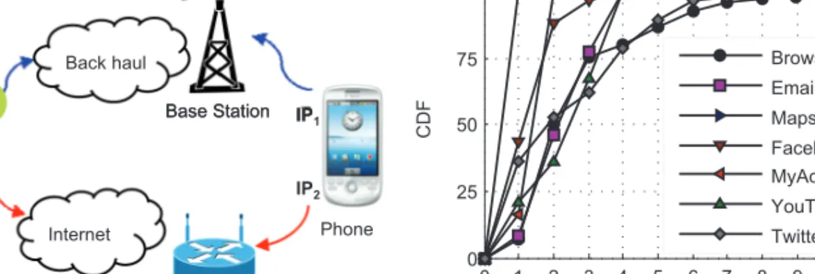
Figure 1 illustrates this problem briefly. An end host, having two interfaces (IP1 and IP2) creates a TCP connection at its port Awith the remote server’s (IP3) port

B. The connection is uniquely identified by the pair (IP1/A,IP3/B). We now analyze what happens if the host decides to turn off its interface,IP1 and wants to continue the communication overIP2. By changing the routes of all outgoing packets, the host may be able to send the next data packets using IP2, but these packets will not be recognized as belonging to the same session at the server, as to the server,IP1andIP2 are two different hosts. If we change the packet headers at the host to carryIP1 as their sources even if they are sent usingIP2, the packets will be either dropped atIP2’s network or even if they get to the server, the ACKs will not reach the host as the server will send ACK toIP1which is closed.

2.2. Potential for Switching Interfaces

A client-based solution that deals with this problem has to wait for all ongoing sessions over the first interface to finish, before it turns off the interface and activates the other one in order to not cause any interruptions. This waiting time can be theoretically infi-nite, but in practice, it depends on the usage of the phone and the characteristics of the applications that are running. To understand the type of data flows in mobile phones, we conduct a 3-month-long experiment to collect the usage data from 13 Android phone users. These users are of different ages, demography, sex, and used a variety of appli-cations. The results are therefore not homogeneous, rather highly diverse as evident later in Figures 15, 16, and 17. The results are also consistent with a 3-month-long study involving 27 iPhone users in Rahmati et al. [2010, 2013].

In our study, the users used a total of 221 applications, and 35 of these applications require Internet connectivity. We analyze the collected data traces of these 35 applica-tions and study the characteristics of the TCP sessions. We study TCP since our earlier work shows that almost all (99.7%) mobile traffic is TCP [Rahmati et al. 2010]. From this log, we try to answer three questions: (1) how many concurrent TCP sessions are there at any instant of time within a mobile phone? (2) what are the durations of these sessions? and (3) how much activities are there over these sessions? Answers to these questions are crucial since if we see that there are a large number of TCP sessions having long durations and high data activities, it is not practical to wait for them and not wise to close them.

Figure 2 shows the cumulative distribution functions (CDF) of concurrent TCP ses-sions of the most popular seven applications in the order of their usages. This is averaged over 10-minutes time windows of all users. This figure has to be studied in conjunction with Figure 3 which classifies these sessions into five classes based on their durations. In Figure 2, we observe that the concurrency of the TCP sessions has

Fig. 1. A phone is trying to switch TCP sessions from 3G(IP1) to WiFi(IP2).

Fig. 2. A steep rise in CDF in between 1–3 indicates that the mean concurrency lies in that interval.

Fig. 3. Applications with high concurrency tend to have most of their sessions with a lifetime of_<15 sec.

Fig. 4. Data activity in long sessions are not con-tinuous, rather they have an average burst length of_∼3 sec.

a steep rise between 1–3. This means that the average value (∼2) lies in this region. Therefore, turning off the interface at any time may interrupt about two sessions on average, assuming that only one application is active at a time. In case of multitasking phones, the number of interruptions is not much higher. Applications like Browser and Twitter seem to show high concurrency (of maximum 10–11), but Figure 3 shows that about 80% of their sessions have a lifetime of<15 seconds. For these applications, we may on average have to wait for 15 seconds before switching to the other interface. Applications like Email, Maps, and T-Mobile’s MyAccount have very high percentage of long-lasting sessions (>120 seconds) which may seem to be a barrier to waiting for them to finish. However, the number of such long TCP sessions is very small (about 1), and with these TCP sessions, the applications keep themselves connected to a specific server (e.g., in case of Google Maps, it is74.125.45.100) for the entire lifetime, and that explains why they are so long.

We conduct further investigation to examine the data activities in these long sessions. Figure 4 shows the presence of data activity of the longest-lasting TCP sessions of each of these applications for a randomly selected user for the first 100 seconds as an example. This shows that, the data activities over these longest TCP sessions are not continuous, but rather sporadic. Averaged over all usages, we see an average of 3-second data activity between any two gaps over these sessions. This indicates that we may have to wait on average about 3 seconds for these applications before switching to a new interface to prevent any data loss. Although this technique will cause that TCP session to terminate, luckily, mobile phone applications are written keeping in mind the sudden loss of network connectivity. Therefore, in such cases, when we switch to a

new interface, the application considers it as a loss of connectivity and re-establishes the connection with the server. We empirically observed this in all 35 applications.

The characteristics of TCP sessions in mobile phones can be summarized as follows: —Average lifetime of TCP sessions is∼2 seconds.

—Average concurrency of these sessions is<2. —TCP activities are in bursts of average∼3 seconds.

—There exist some sessions that are alive during the entire lifetime of the application, which keep the application connected to its server. Disconnections of such sessions are automatically reestablished by the application.

2.3. Switching in MultiNets

MultiNets handles connectionless and connection-oriented sessions separately during switching. UDP and TCP are the dominant transport protocols that we have observed in Android, and therefore we use them in this section for illustrations.

2.3.1. Connectionless Sessions.Connectionless sessions (e.g., UDP) are rare: less than 0.3% of the traffic amount. They are easier to switch. UDP applications communicate using DatagramSocket and each connection is bound to a port and assigned an IP address of an available interface by the OS. To switch the network interface, MultiNets first turns on the new interface and removes the default route over the old interface. We have found that doing so does not affect the functionality of DatagramSocket: the out-bound traffic is sent with the IP of the new interface, while the in-bound traffic is received at the old interface. MultiNets then turns off the old interface, which initially incurs some packet loss of the in-bound traffic, but we have observed that, in most cases, this is handled by the application layer.

2.3.2. Connection-Oriented Sessions.Connection-oriented sessions are mostly TCP, com-prising of about 99.7%. These are trickier to switch as explained earlier. MultiNets performs the following steps for switching these sessions.

Step 1.MultiNets counts the number of ongoing TCP connections on theoldinterface. We should not harm these connections. We exclude the sessions that have gone past the ESTABLISHED state during the counting.

Step 2. If the count is non-zero, MultiNets adds new routing table entries for all these connections explicitly specifying the destination address, gateway, and mask for theoldinterface. This is to ensure that the ongoing TCP sessions still remain in the

oldinterface.

Step 3.MultiNets now brings up thenewinterface and adds routing table entries for it including the default route and removes the default route of theoldinterface from the routing table. Any new connections start using thenewinterface from now on.

Step 4.MultiNets waits for a predefined timeout in order for the ongoing TCP sessions over theoldinterface to finish. Finally, it tears down theoldinterface completely and the system moves on to the new interface.

The users of MultiNets have to configure the WiFi network by providing the authenti-cation information only once. After that, MultiNets switches the interfaces dynamically without requiring any manual intervention. The proposed switching solution in Multi-Nets is fully client based – it does not require additional support from the access points or gateways. Furthermore, MultiNets does not require any modification to the network protocols. It only reads the transport information and adds or removes routing table entries to perform a switch. This is why, existing applications run transparently on MultiNets without any change. There is a possibility that during the Step 4 of the switching, a very long TCP session may get interrupted due to timeout. In Section 5.3,

Fig. 5. Using switchInterface() method to switch to the cellular interface.

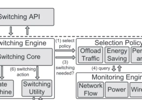
Fig. 6. MultiNets architecture.

we empirically derive a timeout value, for which this interruption becomes a rare phe-nomena. We notice that the proposed switching technique may also be applicable to other applications, for example, Alperovich and Noble [2010] propose a similar tech-nique to switch among homogeneous WiFi access points, and thus is quite different from MultiNets.

2.3.3. Switching API.MultiNets uses the API shown in Figure 5 to switch to a new inter-face. The methodswitchInterface()takes the name of the interface as an argument and returns either success or failure. Upon failure, it throws an exception explaining the reason of failure.

3. DESIGN AND IMPLEMENTATION

The design of MultiNets is modular, consisting of three principal components – Switch-ing Engine,Monitoring Engine, andSelection Policyas shown in Figure 6. These com-ponents isolate the mechanism, policy and monitoring tasks of the system, and allow extending their capabilities without requiring any changes to the architecture.

3.1. The Switching Engine

The Switching Engine performs the switching between cellular and WiFi. It main-tains an internal state machine to keep track of the connectivity status. It also has a Switching Utility module that performs some low-level tasks related to switching. The Switching Core module coordinates these two.

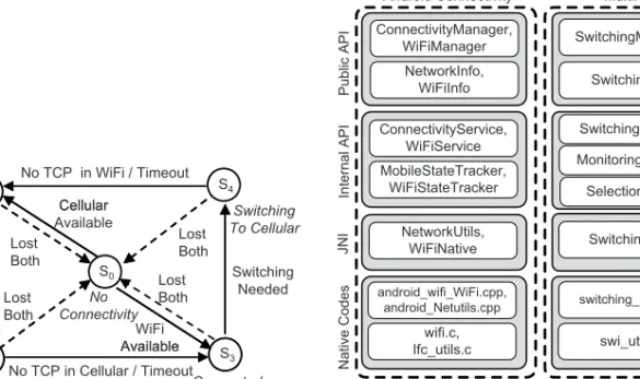
3.1.1. The State Machine.Figure 7 shows the state diagram together with all the states and transitions. The system remains atNoConnectivitystate (S0) when neither cellu-lar nor WiFi is available, and keeps seeking for a network to connect to. The states

ConnectedToCellular(S1) andConnectedToWiFi(S3) are similar. At these states, the device uses only one wireless interface and periodically checks with the Selection Pol-icy (see Section 3.3) to see if a switch is needed. The statesSwitchingToWiFi(S2) and

Fig. 7. State diagram. Fig. 8. Layered implementation.

SwitchingToCellular(S4) are the transition states. Both of the interfaces are active during these states, but only the new connections start over the new interface while existing sessions still remain in the previous interface. The engine stays at these states as long as the old interface has active TCP sessions or until a timeout. Under normal circumstances, the system moves around within the states{S1,S2,S3,S4} circularly. To cope with any loss of connectivity, the system makes transitions shown in dotted arrows. A loss of WiFi connectivity at S2 takes the system to S3, but it immediately starts switching back to cellular upon detecting such a disconnection.

3.1.2. The Switching Utility.The Switching Utility provides the utility methods to per-form the switching. It includes the following tasks – counting the ongoing TCP sessions over a specific network interface; updating the routing table to keep the existing TCP sessions over a specific interface; adding and deleting default routes of the network interfaces; and connecting, reconnecting, or tearing down interfaces. These methods are called by the core switching module to perform a switch.

3.2. The Monitoring Engine

The Monitoring Engine is responsible for monitoring all the necessary phenomena pertaining to switching. It contains several different monitors, each of which observes one or more system variables, and holds the latest value of that variable. We have implemented four monitors – (i)Data Monitor. Monitors the amount of transmitted and received data over WiFi and cellular interfaces in bytes and packets since the interface is turned on, (ii)Wireless Monitor.Monitors the connectivity status, signal strengths, and information of access points, (iii)Network Flow Monitor.Monitors the number and state of all TCP and UDP sessions, routing information from the routing table, and (iv)Power Monitor.Monitors the state of the battery and its voltage, current, and capacity. All these monitors are singleton, that is, there exists only one instance of a monitor in the system. They have a common interface to answer all the queries. The query and its response form a<key, value>pair. The Selection Policy component (see Section 3.3) issues these queries. The modular design of the monitors and a common

interface to talk to them allow us to add new monitors into the system and to easily extend the capability of the existing monitors.

3.3. The Selection Policy

The Selection Policy defines the policy for interface switching. By separating the policies from the rest of the system, we are able to add new policies or modify the existing ones without requiring any change to the other parts of the system. For example, one of our policies is based on the fact that WiFi is much faster than the cellular network. But in the future, this situation may change and cellular data connectivity may outperform WiFi, thereby requiring a change in current policy or adding a new policy. Currently, we have developed and implemented three policies which are described next. Only one of these policies is active at a time. The user of MultiNets determines which policy is used.

3.3.1. Energy-Saving Policy.The aim of this policy is to minimize the power

consump-tion. We describe an optimum energy-saving algorithm in Appendix A, which requires the knowledge of future data traffic. For a realistic setup, we propose a switching heuristic, which is inspired by our energy measurements. According to this policy, the mobile device connects to the cellular network when it is idle, and starts to count the number of bytes sent over the cellular network after the user launches an application. As soon as the total amount of data over the cellular network exceeds a thresholdτ, the device decides to switch to WiFi. The mobile device switches back to the cellular network once the WiFi network is idle forζ seconds. We empirically derive the best τ and ζ values in Section 5.5.1. This policy levarages one fact that the idle power of WiFi is much higher than that of cellular. Techniques such as Ananthanarayanan and Stoica [2009] and Kim et al. [2011] may save some part of the energy that is consumed for scanning WiFi APs– which accounts for about 40% of the idle energy. But even after applying such techniques, WiFi’s idle power remains more than 50 times higher. Hence, switching interfaces dynamically is a better option to save energy.

3.3.2. Offload Policy.The aim of this policy is to offload cellular data traffic to any available WiFi network. According to this policy, whenever WiFi is available, we switch to WiFi. We only switch back to the cellular network when WiFi’s signal strength is below a thresholdηdBm for smooth switching. The advantage of this policy is to reduce data traffic on cellular networks. But the downside is that, if the network is not being used, to keep the WiFi interface idle is more expensive in terms of energy.

3.3.3. Performance Policy.The aim of this policy is to maximize the network

through-put. It achieves this by switching to the network interface with the highest bandwidth. Let, BW(s) and BC(s) be the bandwidth functions for WiFi and cellular networks, re-spectively, wheresdenotes the signal strength, which is read via the Android system API. We empirically derive the bandwidth functions BW(s) and BC(s) in Section 5.5.3 through extensive experiments. The performance policy compares the values of these two functions everyδ seconds, and switches to the network interface with the higher bandwidth.

3.4. Layered Implementation

We have closely studied the software architecture of the data connectivity in Android. Like Android, the implementation of MultiNets is layered. Classes and methods of our system that are similar to those of Android are implemented at the same layer. Yet, our system is vertically distinguishable from Android as shown in Figure 8. At the bottom of the architecture, we have the unmodified Linux Kernel. Right above the Kernel, we have a layer of native C/C++ modules that perform the lower-level tasks

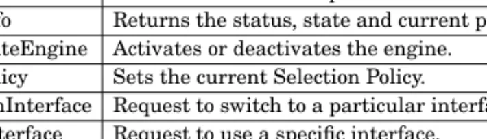
Table I. Descriptions of SwitchingManager API

Method Description

getInfo Returns the status, state and current policy. activateEngine Activates or deactivates the engine. setPolicy Sets the current Selection Policy.

switchInterface Request to switch to a particular interface. useInterface Request to use a specific interface.

of file I/O to get all the information used by the Monitors and some socket I/O to add, remove or update routing table entries. We improve the implementation of Android’s

ifc util.c,route.c, andnetstat.cby adding these nonexisting modules and put them into our own moduleswi utils.c. But no changes are made into the network protocols. These modules are wrapped by JNI and are called from the Internal Classes layer. The Switching Service, Monitoring Service, and Selection Policy are implemented as system services at the Internal Classes layer. These services are created during the device start-up and they run as long as the device is running. We have modified the Android’s System Server to start these services when the device starts. All the changes are done by adding 209 lines of C/C++ code and 650 lines of Java code to Android (Eclair 2.1).

We provide an API to configure and control the Switching Engine which is described in Table I. We use this API to extend Android’s built in wireless control settings appli-cation so that the Switching Engine can be stopped, restarted, and configured to run in different modes from the application layer. When the engine is stopped, this API can also be used by the application programmers to switch interfaces, send a specific flow using a specific interface, or to use multiple interfaces simultaneously. Two of the meth-ods in the API are very useful from the application programmers’ point of view. The first one is, theswitchInterface()method, which allows the programmers to switch inter-faces when needed. This is useful for those kinds of applications that need to send, for example, proprietary data over the cellular network, but for all other purposes prefer to be on WiFi. Another important method is, theuseInterface()method. It is useful to send or receive data using a specific interface for a specific connection. Note that, it does not switch the interface, rather if the preferred network is available, it sends the data using that interface for the specified connection only. With this method, an application can use multiple interfaces simultaneously. In Section 4, we describe this feature in detail.

4. MULTIPLE NETWORK ACCESS

State-of-the-art mobile operating systems maintain static priorities over its network interfaces and always connect to the interface with the highest priority and tear down the interface with a lower priority. The applications cannot choose the network interface by themselves. In contrast, using MultiNets API, applications with proper permissions can request the OS to use a specific interface for communicating with a specific re-mote device. An application notifies MultiNets which interface it wants to use for a remote device. MultiNets then checks whether the interface is available for connectiv-ity, and in case it is available, a route is added into the system routing table for the specific remote IP. Any subsequent TCP or UDP connections are bound to the chosen interface. Figure 9 gives a sample API usage, in which the application transfers sensi-tive data, such as user credentials, over a secured cellular network, and less sensisensi-tive data over a public WiFi network. By using this API, it is also possible to use multiple network interfaces simultaneously for sending and receiving data to separate remote devices.

Fig. 9. Using useInterface() method.

5. EVALUATION

Our evaluation consists of three sets of experiments. First, we measure the system overhead (Section 5.2), switching time overhead (Section 5.3), and energy consumption of interfaces (Section 5.4) to determine the system parameters that are used in the later experiments. Second, we discuss a set of experiments (Section 5.5) that are trace based, where we apply the three policies on the 3-month-long collected data trace to demonstrate the benefits of switching. We also present a video streaming application that uses our API to concurrently activate multiple interfaces. Third, we demonstrate the performance of MultiNets in a real world scenario (Section 5.6).

5.1. Experimental Methodology

5.1.1. Hardware Setup.All experiments are performed on multiple Android Developer

Phones 2 (ADP2) [ADP2 2011]. The mobile devices are running MultiNets which is developed on top of Android OS (Eclair 2.1-update 1). The devices are 3G-enabled T-Mobile phones that use 3G, EDGE, GPRS, and WiFi 802.11 b/g connectivity and are equipped with an 528MHz ARM processor, 512MB flash memory, 192MB RAM, and 1GB microSD card.

5.1.2. Software Setup.We have used benchmarks, data traces from real users, and real

usage of our system as our workloads. We have used a number of benchmarks that are available in the market, such that they as a whole exercise different aspects of the system. Although these benchmarks are useful to evaluate the overhead of the system, we find none of them useful for evaluating the performance of the connectivity of the phone.

Driven by this need, we have developed adata loggerthat is capable of logging ev-ery important information of the running applications within the phone periodically and send it to a remote server. Thirteen volunteers from our research lab, including research scientists, graduate students, faculty, and staffs of age group 25 to 35, were equipped with these phones with our data logger and they carried around the phones to wherever they wanted and used them for both voice and data connectivity for 90 days. The information that we collect from these logs include the names and types of the applications, the frequency and the duration of their usage, and the data usage infor-mation for each wireless interface for each user. For each of these applications, we have the total number of bytes and packets transmitted and received over cellular and WiFi. We modified the Linux’snetstattool for Android to get the information about all the TCP and UDP sessions, which include IP addresses, ports, start time, and durations.

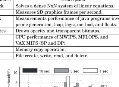
Table II. Description of the Benchmarks

Benchmark Description

Linpack Solves a dense NxN system of linear equations. Fps2d Measures 2D graphics frames per second.

CMark Measurements performance of java programs involving prime generation, loop, logic, method, and floats. Graphics Draws opacity and transparent bitmaps. Cpu CPU performance of MWIPS, MFLOPS, and

VAX MIPS (SP and DP). Mem Memory copy operation.

File File create, write, read, and delete.

Fig. 10. A monitring interval of 5 sec or more keeps the overhead below 5%.

We then implement a traffic generator to reproduce the data sessions. The traffic generator replays the exact same sessions as that are in the log except for that they are now using different server IPs which are situated in our lab instead of the original ones. We load the information about all the sessions into the traffic generator running on the phone and start a process that replays those sessions. As an example, if we want to reproduce Mr. John’s 30 minutes activity of last Friday morning, we just lookup our processed logs to find out the applications that he used during that time window and then instruct each of our servers to mimic one or more of the original servers.

One may argue that instead of collecting the logs and then replaying it, why we do not install and run our engine on the phones in the first place? The answer is that, in order to evaluate the effect of various parameters on our system, or finding the tradeoffs between different parameters of the system, we need to run the engine with the exact same sequence of data activity for different parameter values to cancel out any chance of bias. Therefore, we find this technique useful for generating a realistic and replayable workload for the system evaluation.

5.2. System Overhead

The Switching Engine starts several background system services at the device startup. Running such system services may add additional overhead to the system. The goal of this experiment is to derive a minimal sleeping interval for the monitoring ser-vices so that their overhead is reasonable. We run a set of benchmarks on the device, with and without the Switching Engine and compare the two scores. None of these benchmarks use any data connectivity and, hence, no switching happens during this experiment. The overhead is due to the engine’s continuously monitoring and checking for an opportunity to switch only. We use seven sets of benchmarks that are available in Android Market that has been downloaded 10,000 to 50,000 times. Table II describes the benchmarks.

Figure 10 shows the benchmark scores of the device for running the Switching Engine at 10-, 5-, and 1- second sleeping intervals. The scores are normalized to the scores achieved by a phone running original Android. We see that the longer the sleeping interval, the smaller the overhead and the closer the score is to that of without running

Table III. Lines of Code Lines of code Added Modified

C/C++ 209 0

Java 642 8

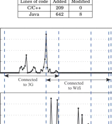
Fig. 11. The top (bottom) figure shows the instantaneous data rate over 3G (WiFi) against the time (sec). Switching from 3G to WiFi starts att1sec when the data rate crosses the 16KBps threshold that we use for this illustration. Both interfaces are active during the switching time [t1,t2], and att2sec, the device completely switches to WiFi. WiFi remains idle during [t3,t4] sec, and switching from WiFi to 3G happens during [t4,t5].

the engine. But if this interval is large, the responsiveness of the engine becomes lazy. We therefore run the engine in 5-second intervals which keeps the overhead below 5% and at the same time the responsiveness is also good. Note that, this overhead is due to the polling style implementation of the monitoring engine and is not an inherent problem of the switching technique itself. A more efficient implementation of the engine is left as our future work. The amount of source code that are added or changed in the original source code of Android is shown in Table III.

5.3. Switching Time

The switching time is the duration between the instant when the engine decides to switch and the instant when it completely connects to the new interface and disconnects the old one. Figure 11 illustrates an example of switching. In this scenario, we start sending data over the 3G, and switch to WiFi when the data rate over 3G exceeds 16 KBps, and switch back to 3G when the WiFi is idle for the last 30 seconds. The timeout for all ongoing TCP sessions over the old interface is set to 20 seconds. The parameters chosen for this experiment are for the demonstration purpose only, they are not set for optimizing anything. The top figure shows the data rate over 3G and the bottom one shows the same for WiFi. We start using 3G for browsing various web pages att0. Att1, when the Monitoring Engine detects that the threshold of 16 KBps is exceeded, the Switching Engine decides to switch to WiFi. It turns on the WiFi connectivity and guides all new sessions to start over WiFi while keeping old sessions

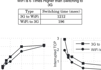
Table IV. Minimum Time to Switch to WiFi is6Times Higher than Switching to

3G

Type Switching time (msec)

3G to WiFi 1212

WiFi to 3G 196

Fig. 12. Timeout value of 30 sec or more makes the switching time ∼15 sec, and keeps the TCP disconnections<1.

active over 3G. This continues tillt2, when the timeout occurs and all existing TCPs over 3G are closed. The duration of [t1,t2], is the switching time during when both the interfaces have one or more active TCP sessions. Aftert2, the phone is connected to WiFi only and continues at this state until it discovers att4that it has been idle since

t3=t4−30s. Att4, the engine again initiates a switching from WiFi to 3G. Since this time we do not have any ongoing TCP over WiFi, the switching to 3G happens almost immediately att5.

Table IV shows the measured switching time overhead. In this case, we do not send or receive any data over any interface. Switching to WiFi takes about 1 second longer than switching to 3G. This is because, connecting to WiFi goes through a number of steps involving scanning for access points, associating with one of them, handshaking and a dhcp request, which are not required for 3G.

Figure 11 reveals that the timeout (20 secs) is the principal component that deter-mines the switching time. To prevent TCP interruptions, we should set the timeout to infinity. But doing so would increase the energy consumption as both interfaces are on during the transition time. Hence, we conduct several experiments to quantify the tradeoff between switching time and number of interrupted TCP sessions.

Figure 12 (left) shows the switching time in presence of data activity for different timeout values. We see that the switching times are closer to the corresponding timeouts for values<5 seconds. As most of the TCP sessions are short-lived and they finish in 10–15 seconds, towards the right of the figure this difference is higher. There are still some sessions that remain till the end of timeout even for values>30 seconds, but they are small in number. Figure 12 (right) plots the number of TCP sessions that gets disconnected against varying timeouts. We see that this number becomes less than 1 after 15 seconds and continues to get lower with increasing values. These long sessions are the ones that the applications use to communicate with their servers and any interruptions of these automatically initiate new connections with the server, and hence there are no visual interruptions for this. Yet, we set the timeout to 30 seconds to reduce the number TCP disconnections and maintain an average switching time of 15 seconds.

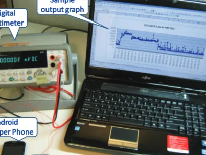
Fig. 13. The digital multimeter, an open battery used for energy measurements, and a sample output graph is shown.

5.4. Energy Measurements

We used a high-precision digital multimeter [Agilent 34410A 2012] to obtain fine-grained energy measurements once every 1 msec as shown in Figure 13. To measure the power drawn by the battery, we opened the battery case to place a 0.1-ohm resistor in series with the battery. The voltage drop across the resistor was used to get the battery current, and this current and the input voltage to the phone were used to calculate the energy consumption. The battery charger was disconnected to eliminate interference from the charging circuitry during this measurement.

We performed energy measurements for data transfers of varying data sizes over 3G and WiFi networks. We measured the energy needed for sending and receiving different data sizes to and from a remote server using HTTP requests. Once a download or upload has been completed, the smartphone sends the next HTTP request to the remote server. Figure 14 shows the average energy consumption for both downloading and upload-ing of 4 KB to 4 MB data over 3G and WiFi networks. Our experiments were performed using a remote server running Linux 2.6.28 with a static IP address located in our lab. We repeated the experiment ten times for each data size and averaged the results. The standard deviation for all these measurements is less than 5%.

For all experiments, we configured the smartphone screen brightness to minimum. We measured the average idle power consumed by the 3G and WiFi network interfaces and found them to be 295.85 mW in case of WiFi and 3.11 mW in case of 3G. In addition, the average energy costs of turning on WiFi and 3G interfaces are 7.19 J and 13.13 J, respectively. We subtract these numbers during the energy measurements in Figure 14 and report only the energy costs for data transfers.

Every data transfer request contains an energy overhead of 12 J for 3G and 1 J for WiFi. After the connection has been established, the energy used to both upload and download is increasing with the amount of data being uploaded or downloaded. These observations are consistent with previous work [Balasubramanian et al. 2009; Rahmati and Zhong 2007]. Figure 14 shows that the energy needed to upload data is higher than that for download since the upload bandwidth is typically smaller.

Fig. 14. Energy consumption during data activity is higher for 3G than WiFi, and uploading is more costly than download.

Fig. 15. Energy-saving heuristic cuts down the av-erage daily energy usage by 27.4% and is close to optimum.

Similarly, because of lower bandwidth of 3G, 3G consumes more energy than WiFi for the same amount of data transfer.

We use the energy measurements for data transfers, turning and keeping on the interfaces to obtain a simple energy model. The energy model is used to estimate the energy for downloading or uploading varying data sizes across 3G and WiFi networks without any other activity on the mobile device. We model the energy cost as follows:

E=EON+ED(d)+P¯ ×(d/R¯), (1) whereEONis the energy to turn on the interface,ED(d) is the energy to transferdbytes of data, ¯Pis the average power to keep the interface on, and ¯Ris the average data rate. We determineED(d) by using linear interpolation and extrapolation on sample points in Figure 14.

5.5. Trace Driven Experiments

5.5.1. Energy Efficiency.Using the energy model, we estimate the average daily

en-ergy consumption for each user in our data traces. We have considered data transfer over WiFi and 3G, and also considered the idle power. We then compute the optimum energy consumption of each user assuming they switched optimally. We use dynamic programming to get this optimum value, which is described in Appendix A. While the algorithm achieves the optimum energy consumption, it assumes that the future data usage is known, which is not realistic. Therefore, in MultiNets, we use a simple heuristic to switch interfaces. As data communication in WiFi is cheaper, for switching from 3G to WiFi, we use a data threshold ofτ KB. If the phone crosses this limit, we switch to WiFi. On the other hand, since idle power of WiFi is much higher than 3G, we switch the phone back to 3G when data activity is absent over WiFi for the last ζ seconds. We systematically tried various τ andζ values using the data traces, and found thatτ =1 KB andζ =60 seconds minimizes the deviation from the optimum en-ergy saving. Therefore, we use these two values throughout the article if not otherwise specified.

Figure 15 shows the average daily energy consumptions of all the users for three strategies: optimum, actual, and the heuristic that we use in MultiNets. This figure shows that switching optimally saves on average 24.17 KJ energy per user per day, which is as high as 89–179 KJ for some users (e.g., 12, 13). We also see that our simple heuristic achieves near-optimal energy consumption with an average deviation of only 13.8%, and we are able to cut down the daily energy usage by 27.4% (21.14 KJ) on average.

Fig. 16. An average of 22.45 MB more data per day per user is offloadable using dynamic switching.

5.5.2. Offloading Traffic.In order to estimate how much data traffic we are able to off-load from 3G to WiFi network with MultiNets, we analyze the data traces that we have collected. For each user, we compute the average daily WiFi usage and compare it to the amount of data that is possible to offload if MultiNets was used. Our offloading strategy is to switch all 3G traffic to WiFi whenever we find a connectible access point. We consider an access point connectible if and only if its signal strength sis above η= −90 dBm and has been used by the user in the past. The threshold−90 dBm is derived from real experiments: when the signal strength is below it, the WiFi is not usable. Figure 16 shows this comparison for each of the users. We see that, for some users (e.g., 3, 7), we are able to offload 11–14 times more data, and for some users who does not tend to use available WiFi at all (e.g., 13) this difference is about 150 MB per day. Considering all users, with switching, we are able to offload on average 22.45 MB of data per day per user which is 79.82% of the average daily usage (28.13 MB).

5.5.3. Performance.Performance of web applications get a significant boost by switch-ing to the interface with the higher bandwidth. In our data trace, we have recorded the signal strengths of both the cellular and all available WiFi networks at 30 seconds intervals. We conduct extensive measurements usingiperftool to find the correlation between signal strengthsand bandwidth B. We runiperfserver on our server, and

iperfclient on Android phones, andiperfpackets traverse through the Internet. We have taken measurements in both indoor and outdoor environments and report the average of 10 measurements at varying signal strengths in Table V. We define the bandwidth functionBW(s) (for WiFi) andBC(s) (for cellular) using linear interpolations on measurement samples in this table.

Using the bandwidth functions, we calculate the average daily throughput of each user for actual usage, and we also do the same if MultiNets was used. Figure 17 shows that, with MultiNets, it is possible to achieve an average throughout of 2.58 MBits/sec, which is 7 times more than the actual usages. For some users (e.g., 1,2,4,13) this gain is about 14–24 times. These are the users who tend to remain in the 3G network even if WiFi is available for them to connect.

Note that, based on our measurement results, even if we take decisions to switch based on the signal strengths, state-of-the-art 3G network being always slower than WiFi, the policy selects WiFi almost as if it were in offload mode. This is, however, not always true, for example, with the rapid advancement of cellular data network technology, this gap is diminishing. Our measurements with recent High Speed Packet Access Network (HSPA+) in Table V shows that this network is about eight times faster than 3G. We believe, in the near future, cellular networks will have a comparable bandwidth to WiFi, and the performance mode of MultiNets will have a higher impact at that moment. Finally, measurement studies report that WiFi throughput may be lower than 3G throughput under certain practical circumstances [Balasubramanian et al. 2010].

Table V. Bandwidth of WiFi, HSPA+, and 3G at Different Signal Levels Measured byiperf

WiFi HSPA+ 3G

Signal Bandwidth Signal Bandwidth Signal Bandwidth (dBm) (Mbps) (dBm) (Kbps) (dBm) (Kbps) ≤ −50 8.58 −65 929 −63 138 (−50,−60] 7.06 −73 858 −89 115 (₋60_,−70] 6_.16 ₋89 746 ₋101 104 (−70,−80] 3.99 −97 509 >−80 1_.25

Fig. 17. The achievable throughput is 7 times higher with switching.

5.5.4. Video Streaming over Multiple Interfaces.Unlike generic applications, video stream-ing services consume high network bandwidth and have strstream-ingent delay constraints, and thus can benefit from concurrently using multiple interfaces [Apostolopoulos and Trott 2004]. Through a real implementation, we demonstrate that MultiNets also sup-ports real-time applications.

We have implemented a streaming server on Linux, which transmits video data using UDP packets to mobile clients. The streaming server supports multipath video streaming for each client, and employs a leaky bucket for every path to control the transmission rate. We have also implemented an Android client using the MultiNets API, which can receive video packets from 3G, WiFi, or both interfaces. The client con-tinuously requests video packets from the server, and periodically reports the average packet loss ratio of each interface to the server. The server adjusts the transmission rates to ensure that the packet loss ratio is below 5% and can be concealed by standard video coding tools [Wang et al. 2000]. The mean packet loss ratio across all experiments is 4.48%.

To faithfully emulate a commercial service, the streaming server is connected to the Internet via a 10Mbps dedicated link, and the mobile phone has two access networks: a 3G network and a WiFi network with residential DSL service. We randomly chose six video traces from a video trace library [Web Page of Video Traces Research Group 2010]. The video traces were extracted from MPEG-4 and H.264/AVC coded streams with diverse video characteristics. We configure the server to stream each video for two minutes, and we instruct the mobile client to log packet arrival times. We repeat the experiments with 3G, WiFi, and both interfaces. We consider two performance metrics:

streaming rateandpreroll delay. Streaming rate refers to the achieved transmission rate, and preroll delay is the time for the client to fill its receiving buffer in order to guarantee smooth playout.

We plot streaming rates in Figure 18, which shows that the streaming service achieves higher streaming rates by using both interfaces. More precisely, compared to WiFi and 3G, streaming over both interfaces increases the streaming rate by 43% and 271%, respectively. Table VI presents the preroll delays of three high-resolution

Fig. 18. Streaming with both interfaces leads to higher streaming rate. Table VI. Streaming with Both Interfaces Achieves Lower Preroll

Delay

Preroll Delay Matrix (sec) StarWar (sec) Olympic (sec)

3G 195.50 77.42 477

WiFi 20 1.36 117

3G & WiFi 0.16 0.15 51

videos; other videos have much lower encoding rates and require negligible preroll delays. Table VI illustrates that streaming over both interfaces significantly reduces the preroll delay, for example, the preroll delay of Matrix is reduced from 195.5 sec-onds (or 20 secsec-onds) to merely 0.16 seconds by using both interfaces. Higher streaming rates and lower preroll delays lead to better user experience, which is made possible by MultiNets.

5.6. Real Deployment

To quantify the performance of our system in a real-world scenario, we conduct actual experiments at the Stanford University campus. We have chosen this campus since it has WiFi connectivity both inside and outside of the buildings and also has several areas where WiFi is either completely unavailable or has a very poor signal strength. High availability of WiFi is important for us since we want to demonstrate that our system is switching back to 3G to conserve energy even in presence of WiFi. On the other hand, loss and reconnection of WiFi connectivity is important to demonstrate that our system is capable of switching smoothly. We take four ADP2 phones with us. Two of these have our system installed and the other two run Android (Eclair 2.1). All four phones are fully charged and their screen brightnesses are set to the lowest level. For a fair comparison, we use our traffic generator to replay the same data traffic in all of them. The traffic generator runs in the phone and sends and receives data over the Internet to and from our server which is situated in our lab at 4 miles distant from Stanford. The phones replay the traffic patterns of the most popular six applications from our data traces having sessions of varying numbers, durations, delays, and concurrencies. Once started, the phones run each of these applications for 10 minutes followed by a 10-minute break, repeatedly one after the other. We log the transmitted and received bytes, signal strengths, MAC addresses of WiFi APs, battery current, voltage and capacity into the file system of the phone periodically every 2 seconds for later analyses.

5.6.1. Energy Efficiency.In this experiment, we configure one of our phones into the

energy-saving mode. We take another two phones that run Android – one with WiFi enabled, and the other staying over 3G only. We start the traffic generator in all three phones and begin our 168-minute campus tour starting from the Computer Science building. We move around all five floors of the building for an hour, then take an

Fig. 19. We encounter 37 WiFi APs, average signal strengths of−68.46 dBm (inside) and−82.34 dBm (outside), and 28 WiFi disconnections during the tour.

Fig. 20. Energy saving mode saves about 28.4%–33.75% energy as compared to Android.

hour-long round-trip tour within the campus as shown in Figure 19, and finally get back to the building to spend the rest of the tour. During this tour, we encounter 37 different WiFi APs, an average signal strength of−68.46 dBm inside the building and

−82.34 dBm outside the building, 28 disconnections from WiFi to 3G, and a total of 49 switchings by our system. Using the instantaneous values of current and voltage obtained from the log, we compute the energy consumption of each of these phones and plot the cumulative energy consumption in Figure 20. Despite the fact that the battery voltages and currents read from the Android system are not in high precision, we still see a clear difference of the energy consumption among these three phones. We see that for the same data traffic, our system achieves about 28.4%–33.75% energy savings as compared to the state-of-the-art Android systems.

5.6.2. Offloading and Throughput.In this experiment, we compare the offloading and

throughput of our system with that of the state-of-the-art Android. In MultiNets, we set the switching timeout to be 30 seconds. Recall that, cellular network being much slower than WiFi, the outcomes of Offload and Performance modes are similar, although their decision mechanisms are completely different. Therefore, we present them together in Table VII. This table also gives the achievable lower and upper bounds of Android

Table VII. For Near-Optimal Offloading and Throughput, MultiNets Experiences no TCP Disconnections Thought the Experiments

System Offload (MB) Throughput (kbps) Disconnections (Count)

MultiNets 45.41 116.20 0

Android (3G Only) 0 39.29 0

Android (WiFi ON) 44.54 116.26 8

Table VIII. Energy-Saving Mode Saves55_.85%More Energy, but Sacrifices14.25%Offloading

Mode Energy Consumption (J) Offload (MB)

Energy Saving 90.36 38.94

Offload 204.65 45.41

on offloading and throughput. The lower bound is derived by disabling WiFi interface (3G Only), and the upper bound is achieved by always switching to WiFi whenever it is available (WiFi ON). This table shows that: MultiNets (i) leads to three times higher throughput than the Android lower bound, (ii) achieves near-optimal offloading and throughput, and (iii) experienceszeroTCP disconnections throughout the experiments, while Android upper bound results ineightTCP disconnections.

5.6.3. Energy Efficiency vs. Offload Tradeoff.It is interesting to see the tradeoffs between the energy savings and offloading. Table VIII shows that, MultiNets in energy-saving mode consumes about 55.85% less energy than offload mode, but sacrifices about 14.25% of offloading capability. The reason behind this is that energy-saving mode keeps the phone in 3G while it is idle. When data transmission starts, it keeps the phone in 3G mode for a while before completely switching to WiFi, and hence the overall WiFi offloading is slightly lower in this case. This experiment illustrates that, users of MultiNets achieve different objectives by putting the system in different modes.

6. RELATED WORK

Switching among multiple network interfaces of a mobile device has been considered in the literature. However, all the prior proposals require either new network infras-tructure or new network protocols, and thus are not widely deployed in the Internet. In contrast, we design and implement practical OS support to realize dynamic network traffic distribution without new infrastructure and protocol. Our solution can work with various optimization criteria yet be totally transparent to existing applications. It can also be tightly integrated with applications with strict Quality-of-Service (QoS) re-quirements, for example, real-time video streaming systems. The previously proposed solutions can be categorized into three groups.

—Protocol.New protocols in various layers have been designed to support switching among access networks. Wang et al. [2007] propose a rate control algorithm for mul-tiple access networks, which needs to be integrated into application-layer protocols. Kim and Copeland [2003] and Wu et al. [2007] propose TCP variants that result in better performance by switching among access networks. Mobile IP [Perkins 1997] uses foreign/home agents to forward network traffic from/to a smartphone that move among access networks. Such traffic forwarding increases traffic load on agents and incurs additional network latency. Mobile IP v6 [Nikander et al. 2003] uses optimized routes for lower network latency, but it still relies on deploying foreign/home agents for mobility management. In contrast to MultiNets, widely deploying TCP variants and mobile IP agents in the Internet incurs tremendous costs and burden, and may take years to be done.

—Gateway.Gateways between smartphones and the Internet can be used for accessing multiple network interfaces. Balasubramanian et al. [2010] design a system to reduce the network traffic over cellular networks by switching between cellular and WiFi networks. More specifically, it transmits delay tolerant data over WiFi networks, which may not be always available, and real-time data over cellular networks, which have better coverage. Sharma et al. [2004] propose a system that uses gateways to aggregate network resources from multiple access networks among several collab-orative smartphones. Armstrong et al. [2006] uses a proxy to notify the phone via sms about content updates and suggests interface to use. Unlike MultiNets, gateway solutions require deploying expensive gateways, incurs additional network latency, and may need users to configure the proxy settings in applications.

—Master/slave. A master/slave solution [Pahlavan et al. 2000] chooses an always-connected access network as the master network, and uses other access networks as slave networks for opportunistic routing. While control traffic always goes through the master network, data traffic is offloaded via slave networks whenever they are available. Different from MultiNets, deploying master/slave solutions requires com-plete control over multiple access networks, which is difficult due to business reasons. Higgins et al. [2010] propose intentional networking where applications provide hints to the system and system chooses the best interface opportunistically. In contrast, MultiNets is completely transparent to the existing applications.

Last, Rahmati et al. [2013] demonstrate the feasibility of TCP flow migration on iPhones, but they do not address or rigorously quantify the policies and different bene-fits of switching interfaces. A preliminary version of MultiNets was presented in Nirjon et al. [2012]; more details are given in the current article.

7. CONCLUSION AND FUTURE WORK

In this article, we consider the problem of real-time switching between multiple net-work interfaces on mobile devices. We first conduct a three-month-long empirical study to understand the TCP characteristics on Android devices. Based on this study, we de-sign a client-based solution to the switching problem. We then present the MultiNets system that uses this technique to switch dynamically between WiFi and cellular networks based on three policies: energy efficiency, offloading data traffic, and higher throughput. Our evaluation results show that our system outperforms the state-of-the-art Android either by saving up to 33.75% energy, or achieving near-optimal offloading, or achieving near-optimal throughput while substantially reducing TCP interruptions due to switching. Moreover, our system also allows resource-demanding applications to concurrently activate both network interfaces. Although our implementation is An-droid based and considers only two types of networks: WiFi and cellular, the same technique and principle is applicable to any mobile OS’s and extensible to any number of interfaces. With the growing number of wireless protocols and support for multi-ple radios in mobile devices, most future systems will adopt this concept of interface switching to achieve a better efficiency in network access.

We emphasize that MultiNets is general and can work with different selection poli-cies. While the three sample policies presented in this article might look a bit simple at first glance, readers can always define new selection policies for potentially better out-comes at the expense of higher complexity. For example, the performance policy (see Section 3.3.3) predicts the wireless network throughput using signal strength only, which may be less accurate than using both the signal strength and congestion level. However, measuring the congestion level of wireless networks itself is a challenging issue [Acharya et al. 2008], and is out of the scope of this article. Last, we note that our current selection policies employ models trained offline. As one of our future tasks,

we plan to develop online models for the selection policies, which adapt to the dynamic environments on-the-fly. We also plan to study the possibility of employing crowdsourc-ing [Yuen et al. 2011] to collect more samples for model traincrowdsourc-ing, in order to shorten the training time and increase the model accuracy.

APPENDIX

A. OPTIMUM ENERGY COMPUTATION

Given, the data usage Di of a user for every T seconds, energy for turning on (EW_ON,

EC

ON), data transfer (EWD(Di), EDC(Di)), and idle power (PW, PC) of the WiFi and cellu-lar, and the availability of WiFi, our goal is to find the optimum energy consumption considering switching. The problem is an instance of classical multistage graph op-timization problem where the time points are the stages and the interfaces are the choices (sometimes only one choice of 3G) at each stage. Let us define f(i,C) as the optimum energy from the starting time (time=1) tillith time such that we use 3G at timei. The definition of f(i,W) for WiFi is similar. We now formulate the following recurrence relations: f(i,C)=min f(i−1,C)+PC_{×T +E}C D(Di) f(i−1,W)+EC ON+P C_{×T +E}C D(Di), and f(i,W)=min f(i−1,W)+PW×T +E_DW(Di) f(i−1,C)+EW ON+PW×T +EWD(Di), where the initial conditions are f(0,C)=EC

ON, f(0,W)=EWON. These recurrences are written assuming WiFi is available. To address the cases when WiFi is not available, we ignore f(i−1,W) in f(i,C), and make f(i,W)= f(i,C). Finally, the optimum energy is computed as the minimum of f(n,W) and f(n,C) wherenis the total number of time points.

REFERENCES

Agilent. 2012. Agilent 34410A digital multimeter. http://cp.literature.agilent.com/litweb/pdf/34410-90001. pdf.

P. Acharya, A. Sharma, E. Belding, K. Almeroth, and K. Papagiannaki. 2008. Congestion-aware rate adapta-tion in wireless networks: A measurement-driven approach. InProceedings of the IEEE Communications Society Conference on Sensor, Mesh and Ad Hoc Communications and Networks (SECON’08). 1–9. ADP2. 2011. Android developer phone 2 (ADP2). http://web.archive.org/web/20110712230222/http://

developer.htc.com/google-io-device.html.

T. Alperovich and B. Noble. 2010. The case for elastic access. InProceedings of the ACM 5th International Workshop on Mobility in the Evolving Internet Architecture (MobiArch’10). ACM.

G. Ananthanarayanan and I. Stoica. 2009. Blue-fi: Enhancing wi-fi performance using bluetooth signals. InProceedings of the ACM 7th International Conference on Mobile Systems, Applications, and Services (MobiSys’09).

J. Apostolopoulos and M. Trott. 2004. Path diversity for enhanced media streaming.IEEE Commun. Mag. 42, 80–87.

T. Armstrong, O. Trescases, C. Amza, and E. Lara. 2006. Efficient and transparent dynamic content up-dates for mobile clients. InProceedings of the ACM 4th International Conference on Mobile Systems, Applications, and Services (MobiSys’06).

AT&T. 2009. AT&T faces 5,000 percent surge in traffic. http://www.internetnews.com/mobility/article. php/3843001.

A. Balasubramanian, R. Mahajan, and A. Venkataramani. 2010. Augmenting mobile 3G using WiFi. In Proceedings of the ACM 8th International Conference on Mobile Systems, Applications, and Services (MobiSys’10).