Multi-line distance minimization: A visualized many-objective test problem suite

Multi-Line Distance Minimization: A Visualized

Many-Objective Test Problem Suite

Miqing Li, Crina Grosan, Shengxiang Yang,

Senior Member, IEEE

, Xiaohui Liu, and Xin Yao,

Fellow, IEEE

Abstract—Studying the search behavior of evolutionary

many-objective optimization is an important, but challenging issue. Existing studies rely mainly on the use of performance indica-tors which, however, not only encounter increasing difficulties with the number of objectives, but also fail to provide the visual information of the evolutionary search. In this paper, we propose a class of scalable test problems, called multi-line distance minimization problem (ML-DMP), which are used to visually examine the behavior of many-objective search. Two key characteristics of the ML-DMP problem are: 1) its Pareto optimal solutions lie in a regular polygon in the two-dimensional decision space, and 2) these solutions are similar (in the sense of Euclidean geometry) to their images in the high-dimensional objective space. This allows a straightforward understanding of the distribution of the objective vector set (e.g., its uniformity and coverage over the Pareto front) via observing the solution set in the two-dimensional decision space. Fifteen well-established algorithms have been investigated on three types of 10 ML-DMP problem instances. Weakness has been revealed across classic multi-objective algorithms (such as Pareto-based, decomposition-based and indicator-decomposition-based algorithms) and even state-of-the-art algorithms designed especially for many-objective optimization. This, together with some interesting observations from the experimental studies, suggests that the proposed ML-DMP may also be used as a benchmark function to challenge the search ability of optimization algorithms.

Index Terms—Many-objective optimization, evolutionary

algo-rithms, test problems, visualization, search behavior examination.

I. INTRODUCTION

E

Manuscript received Match 15, 2016; revised July 24, 2016 and November 7, 2016; accepted January 4, 2017. This work was supported in part by the Engineering and Physical Sciences Research Council (EPSRC) of U.K. under Grants EP/K001523/1 and EP/K001310/1, National Natural Science Founda-tion of China (NSFC) under Grants 61329302, 61403326 and 61673331. X. Yao was also supported by a Royal Society Wolfson Research Merit Award. M. Li and X. Yao are with the Centre of Excellence for Research in Computational Intelligence and Applications (CERCIA), School of Computer Science, University of Birmingham, Birmingham B15 2TT, U. K. (e-mail: [email protected], [email protected]).

C. Grosan is with the Department of Computer Science, Brunel Uni-versity London, Uxbridge UB8 3PH, U. K. and also with the Department of Compuer Science, Babes-Bolyai University, Cluj Napoca, Romania (e-mail: [email protected]).

S. Yang is with the School of Computer Science and Informatics, De Montfort University, Leicester LE1 9BH, U. K. (e-mail: [email protected]). X. Liu is with the Department of Computer Science, Brunel University London, Uxbridge UB8 3PH, U. K. (e-mail: [email protected]).

However, search behavior examination can be challenging in the context of evolutionary multi-objective optimization (EMO). For a multi-objective optimization problem (MOP), there is often no single optimal solution (point) but rather a set of Pareto optimal solutions (Pareto optimal region). We may need to consider not only the convergence of the evolutionary population to these optimal solutions but also the representativeness of the population to the whole optimal region. This becomes even more difficult when an MOP has four or more objectives, usually called a many-objective optimization problem [1]–[3]. In many-objective optimization, the observation of the evolutionary population by the scatter plot, which is the predominating, most effective visualization method in bi- and tri-objective cases, becomes difficult to comprehend [4]–[8].

In the EMO community, there exist several test problem suites available for many-objective optimization. Among these, DTLZ [9] and WFG [10] are representations of continuous problem suites, and Knapsack [11], TSP [12] and MNK-Landscapes [13] are representations of discrete ones. Recently, researchers have also presented several new MOPs for many-objective optimization [14]–[16]. The above test problems have their own characteristics, and some of them have been widely used to examine the performance of many-objective evolutionary algorithms [17]–[26]. In the performance exam-ination, an algorithm is called on a test problem and then returns a set of solutions with high dimensions.

How to assess such a solution set is not a trivial task. The basic way is to resort to performance indicators. Unfortunately, there is no performance indicator that is able to fully reflect the search behavior of evolutionary algorithms. On the one hand, it is challenging to find (or design) a performance indicator suited well to many-objective optimization, as a result of growing difficulties with the number of objectives, such as the requirement of time and space complexity, ineffectiveness of the Pareto dominance criterion, sensitivity of the parameter settings, and inaccuracy of the Pareto front’s substitution. Many performance indicators that are designed in principle for any number of objectives may be invalid or infeasible in practice in many-objective optimization [27].

On the other hand, one performance indicator only examines one specific aspect of algorithms’ behavior. Even those perfor-mance indicators that aim to examine the same aspect of the population performance also have their own preference. For example, two commonly used indicators, inverted generational distance (IGD) [28] and hypervolume (HV) [11], both of which provide a combined information of convergence and diversity of the population, can bring inconsistent assessment

results [29]–[31]. For two populations being of same conver-gence, IGD, which is calculated on the basis of uniformly distributed points along the Pareto front, prefers the one having uniformly distributed individuals, while HV, which is typically influenced more by the boundary individuals, has a bias towards the one having good extensity.

More importantly, performance indicators cannot provide the visual information of the evolutionary search. This matters, especially for researchers and practitioners with the real-world application background who typically have no expertise in the EMO performance assessment – it could be hard for them to understand the behavior of EMO algorithms only on the basis of the returned indicator values.

Recently, EMO researchers introduced a class of test prob-lems (called the multi-point distance minimization problem (MP-DMP)1[37]) for visual examination of the search behav-ior of multi-objective optimizers. As its name suggests, the MP-DMP problem is to simultaneously minimize the distance of a point to a pre-specified set (or several pre-specified sets) of target points. One key characteristic of MP-DMP is its Pareto optimal region in the decision space is typically a 2D manifold (regardless of the dimensionality of its objective vectors and decision variables). This naturally allows a direct observation of the search behavior of EMO algorithms, e.g., the convergence of their population to the Pareto optimal solutions and the coverage of the population over the optimal region.

Over the last decade, the MP-DMP problem and its variants have gained increasing attention in the evolutionary multi-objective (esp. many-multi-objective) optimization area. K¨oppen and Yoshida [33] constructed a simple MP-DMP instance which minimizes the Euclidean distance of a point to a set of target points in a 2D space. This leads to the Pareto optimal solutions residing in the convex polygon formed by the target points. Rudolph et al. [38] introduces a variant of MP-DMP whose Pareto optimal solutions are distributed in multiple symmetrical regions in order to investigate if EMO algorithms are capable of detecting and preserving equivalent Pareto subsets. Sch¨utze et al. [39] and Singh et al. [40] used the MP-DMP problem to help understand the characteristics of many-objective optimization, analytically and empirically, respectively. Ishibuchi et al. [41] generalized the MP-DMP problem and introduced multiple Pareto optimal polygons with same [41] or different shapes [42]. Later on, they examined the behavior of EMO algorithms on the MP-DMP problem with an arbitrary number of decision variables [34], and also further generalized this problem by specifying reference points on a plane in the high-dimensional decision space [43]. Very recently, Zille and Mostaghim [35] used the Manhattan distance measure in MP-DMPs and found that this can drastically change the problem’s property and difficulty. Xu et al. [36] proposed a systematic procedure to identify Pareto optimal solutions of the MP-DMP under

1_{The multi-point distance minimization problem has different names or}

abbreviations in the literature (such as the Pareto box problem [32], P∗

problem [33], distance minimization problem [34], DMP [35], and M-DMP [36]). For the contrast of the work presented in this paper, we abbreviate it as MP-DMP here.

the Manhattan distance measure and also gave a theoretical proof of their Pareto optimality. Fieldsend [44] embedded dominance resistance regions into the MP-DMP problem and demonstrated that Pareto-based approach can be fragile to dominance resistance points. Overall, the MP-DMP problems present a good alternative for researchers to understand the behavior of multi-objective search. Consequently, they have been frequently used to visually compare many-objective optimizers in recent studies [45]–[47].

However, one weakness of the MP-DMP problem is its inability to facilitate examination of the search behavior in the objective space. There is no explicit (geometric) similarity relationship between decision variables’ distribution and that of objective vectors. Even when a set of objective vectors are distributed perfectly over the Pareto front, we cannot know this fact via observing the corresponding solution variables in the decision space.

As the first attempt to solve the above issue, we recently presented a four-objective test problem whose Pareto optimal solutions in the decision space are similar (in the sense of Euclidean geometry) to their images in the objective space [48]. This therefore allows a straightforward understanding of the behavior of objective vectors, e.g., their uniformity and coverage over the Pareto front. However, to comply to the geometric similarity between the Pareto optimal solutions and their objective images, the presented problem fixes its objective dimensionality to four. This makes it impossible to examine the search behavior of EMO algorithms in a higher-dimensional objective space.

In this paper, we significantly extend our previous work in [48] and propose a class of test problems (called the multi-line distance minimization problem, ML-DMP) whose objective dimensionality is changeable. In contrast to the MP-DMP which minimizes the distance of a point to a set of target points, the proposed ML-DMP minimizes the distance of a point to a set of target lines. Two key characteristics of the ML-DMP are that its Pareto optimal solutions 1) lie in a regular polygon in the two-dimensional decision space and 2) are similar (in the sense of Euclidean geometry) to their images in the high-dimensional objective space. In addition to these, the ML-DMP has the following properties.

• It is scalable with respect to the number of objectives –

its objective dimensionality can be set by the user freely.

• Its difficulty level is adjustable, which allows a viable

ex-amination of diverse search abilities of EMO algorithms.

• It provides an interesting dominance structure which

varies with the number of objectives, e.g., for the four-objective instance there exist some areas dominated only by one line segment and for the five-objective one there exist some areas dominated only by one particular point. The paper conducts a theoretical analysis of the geometric similarity of the Pareto optimal solutions and also of their optimality in the polygon as to the given search space. For experimental examination, the paper considers 10 instances of the ML-DMP problem with 3, 4, 5, and 10 objectives and investigates the search behavior of 15 well-established algo-rithms on these instances. This investigation provides a visual

Y

X

Fig. 1. A tri-objective ML-DMP instance where A1,A2 andA3 are the three vertexes of the regular triangle.

understanding of the search behavior of EMO algorithms on different objective dimensionality and varying search space.

The rest of this paper is structured as follows. Section II describes the proposed ML-DMP and this includes an analysis of the problem’s geometric similarity and Pareto optimality. Section III introduces experimental design. Section IV is devoted to experimental results. Finally, Section V draws conclusions and gives possible lines of future work.

II. MULTI-LINEDISTANCEMINIMIZATIONPROBLEM (ML-DMP)

The multi-line distance minimization problem considers a two-dimensional decision space. For any point P = (x, y) in this space, the ML-DMP calculates the Euclidean distance from P to a set of m target straight lines, each of which passes through an edge of the given regular polygon with m vertexes(A1, A2, ..., Am), wherem≥3. The goal in the

ML-DMP is to optimize these m distance values simultaneously. Fig. 1 gives a tri-objective ML-DMP instance.A1,A2andA3 are the three vertexes of a regular triangle, and←−−→A1A2,←−−→A2A3 and←−−→A3A1 are the three target lines passing through the three edges of the triangle. Thus, the objective vector of a pointP is (f1, f2, f3) = (d(P,←−−→A1A2), d(P,←−−→A2A3), d(P,←−−→A3A1)), where d(P,←−→AiAj) denotes the Euclidean distance from pointP to

straight line←−→AiAj.

It is clear that there does not exist a single point P on the decision space that can reach minimal value for all the objectives. For the tri- or four-objective ML-DMP, the Pareto optimal region is their corresponding regular polygon. But this may not be the case for the ML-DMP with five or more objectives. The identification of the Pareto optimal solutions of the ML-DMP will be presented in the later part of this section (Section II-B).

A. Geometric Similarity of the ML-DMP

An important characteristic of the ML-DMP is that the points in the regular polygon (including the boundaries) and their objective images are similar in the sense of Euclidean geometry. In other words, the ratio of the distance between

-1.0 -0.5 0.0 0.5 1.0 -0.5 0.0 0.5 1.0 Y X

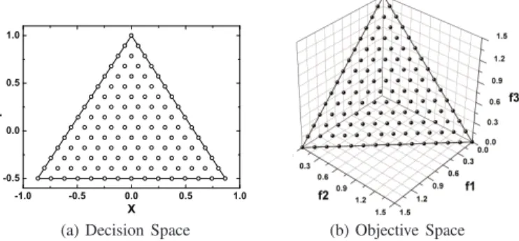
(a) Decision Space (b) Objective Space Fig. 2. An illustration of geometric similarity of the ML-DMP on a tri-objective instance, where a set of uniformly-distributed points over the regular triangle in the decision space lead to a set of uniformly-distributed objective vectors.

any two points in the polygon to the distance between their corresponding objective vectors is a constant. Fig. 2 illustrates the geometric similarity between the polygon points and their images on a tri-objective ML-DMP. Next, we give the definition of the geometric similarity for an ML-DMP with any number of objectives.

Theorem 1. For an ML-DMP problem, the Euclidean distance between any two solutions that lie inside the regular polygon (including the boundaries) is equal to the Euclidean distance between their objective images multiplied by a constant. For-mally, for any two interior solutionsP1(x1, y1)andP2(x2, y2) of the polygon of an ML-DMP problemF = (f1, f2, ..., fm),

we have

||P1−P2||=k||F(P1)−F(P2)||

which can be rewritten as

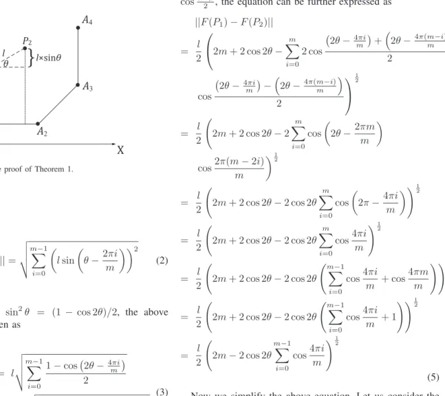
p (x1−x2)2−(y1−y2)2=k v u u t m X i=1 (fi(P1)−fi(P2))2 (1) Proof:Let us consider the notations as in Fig. 3. Without loss of generality, it can be supposed that one edge of the polygon (for instance A1A2) is parallel with X axis and P1 andP2 are two points inside the polygon. Let us denote byθ the angle between the line←−→P1P2 andXaxis. Then

f1(P1)−f1(P2) = d(P1,A←−−→1A2)−d(P2,←−−→A1A2) = lsinθ

where l is the Euclidean distance between P1 and P2 (i.e.,

||P1−P2||=l).

Since the polygon is regular, the same property holds for the edge←−−→A2A3, with the difference that the angle between←−−→A2A3 andXaxis is 2π/m. Thus, we have

f2(P1)−f2(P2) = d(P1,A←−−→2A3)−d(P2,←−−→A2A3) = lsin(θ−2π/m)

This can be visualized as rotating the coordinate system with 2π/m degrees, when the angle between the line ←−→P1P2 andX axis in the new coordinate system isθ−2π/m. Now

Y

A

X

A

A

A

Fig. 3. Illustration for the proof of Theorem 1.

we further have ||F(P1)−F(P2)||= v u u t m−1 X i=0 lsin θ−2πi m 2 (2)

Using the relation sin2θ = (1 − cos 2θ)/2, the above equation can be written as

||F(P1)−F(P2)||= l v u u t m−1 X i=0 1−cos 2θ−4πi m 2 = √l 2 v u u tm− m−1 X i=0 cos 2θ−4_mπi (3)

If we change the index of the sum fromi= 0,1, ..., m−1to i= 0,1, ..., m−1, mand use the relationcos(2θ−4πm/m) = cos 2θ, the equation can be expressed as

||F(P1)−F(P2)|| = √l 2 m+ cos 2θ− m X i=0 cos 2θ−4_mπi ! 1 2 = l 2 2m+ 2 cos 2θ−2 m X i=0 cos 2θ−4_mπi ! 1 2 = l 2 2m+ 2 cos 2θ− m X i=0 cos 2θ−4_mπi + cos 2θ−4π(m_m−i) 12 (4)

According to the relation cosα+ cosβ = 2 cosα+₂β ·

cosα−β

2 , the equation can be further expressed as

||F(P1)−F(P2)|| = l 2  2m+ 2 cos 2θ− m X i=0 2 cos 2θ−4πi m +2θ−4π(m−i) m 2 cos 2θ− 4πi m −2θ−4π(m−i) m 2   1 2 = l 2 2m+ 2 cos 2θ−2 m X i=0 cos 2θ−2πm_m cos2π(m−2i) m 12 = l 2 2m+ 2 cos 2θ−2 cos 2θ m X i=0 cos 2π−4πi m ! 1 2 = l 2 2m+ 2 cos 2θ−2 cos 2θ m X i=0 cos4πi m !12 = l 2 2m+ 2 cos 2θ−2 cos 2θ m−1 X i=0 cos4πi m + cos 4πm m !!12 = l 2 2m+ 2 cos 2θ−2 cos 2θ m−1 X i=0 cos4πi m + 1 !!12 = l 2 2m−2 cos 2θ m−1 X i=0 cos4πi m !12 (5) Now we simplify the above equation. Let us consider the complex numberω=cos4_mπ+isin4_mπ. Thenωx_{= cos}4πx

m +

isin4_mπx andωm_{= cos}4πm m +isin

4πm

m =cos 4π+isin 4π=

1. We know thatωm_{−1 = 0. Thus(ω−1)(ω}m−1_+ωm−2₊

· · ·+ω+ 1) = 0. Sinceω6= 1, it holdsωm−1_+ωm−2_{+· · ·+}

ω+ 1 = 0, which means thatPm−1

i=0 (cos4mπi+isin

4πi m) = 0.

This indicates that both real and imaginary parts equal0. Thus

m−1

X

i=0

cos4πi m = 0 If we now go back to Eq. (5), we have

||F(P1)−F(P2)|| = l 2 2m−2 cos 2θ m−1 X i=0 cos4πi m !12 = l 2 √ 2m=l r m 2 (6) Since||P1−P2||=l, we finally have

||P1−P2||=

r

2

m||F(P1)−F(P2)|| (7) where m is the problem’s objective dimensionality. This completes the proof of Theorem 1.

Note that the polygon of the ML-DMP should be regular; otherwise, this theorem does not hold.

B. Pareto Optimality of the ML-DMP

To consider the Pareto optimality of the ML-DMP, let us first recall several well-known concepts in multi-objective opti-mization: Pareto dominance, Pareto optimality, Pareto optimal set and Pareto front. Without loss of generality, we consider the minimization MOP here.

Definition 1 (Pareto dominance). For an MOP F(P) = (f1(P), f2(P), ..., fm(P)), let P1 and P2 be two feasible solutions (denoted as P1, P2 ∈ Ω). P1 is said to Pareto dominateP2 (denoted asP1≺P2), if and only if

∀i∈(1,2, ..., m) :fi(P1)≤fi(P2)∧

∃j∈(1,2, ..., m) :fj(P1)< fj(P2) (8)

On the basis of the concept of Pareto dominance, the Pareto optimality and Pareto optimal set (Pareto front) can be defined as follow.

Definition 2 (Pareto optimality). A solution P∗ _{∈Ω is said}

to be Pareto optimal if there is no P ∈Ω,P≺P∗_.

Definition 3(Pareto optimal set and Pareto front). The Pareto optimal set is defined as the set of all Pareto optimal solutions, and the Pareto front is the set of their corresponding images in the objective space.

Next, we discuss the Pareto optimal solutions of the ML-DMP problem.

Theorem 2. For an ML-DMP (Ω = R2) with a regular polygon of m vertexes (A1, A2, ..., Am), points inside the

polygon (including the boundary points) are the Pareto optimal solutions. In other words, for any point in the polygon, there is no point _∈R2 that dominates it.

Proof: See Section I in the Supplement of the paper. This theorem indicates that all points inside the polygon are the Pareto optimal solutions. However, these points may not be the sole Pareto optimal solutions of the problem. That is, there may exist some points outside the polygon that are not dominated by these points.

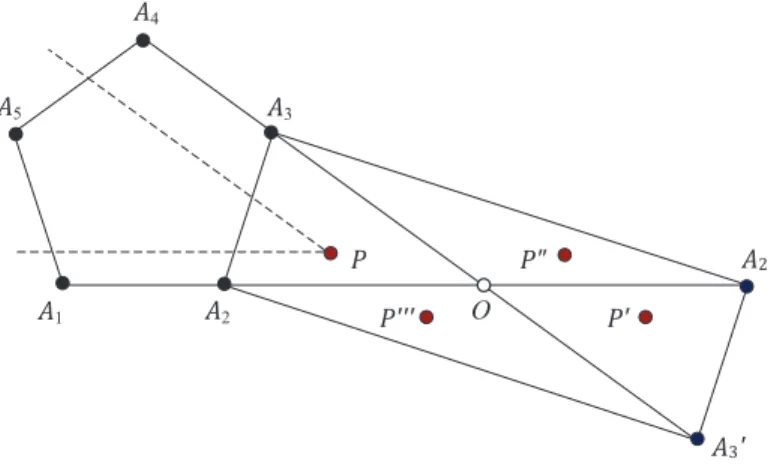
Consider a five-objective ML-DMP in Fig. 4, whereA1 to A5 are the five vertexes of the regular pentagon. Point O is the intersection point of the two target lines←−−→A1A2and←−−→A4A3, andA′

2 andA′3 are the symmetric points of A2 andA3 with respect to point O, respectively. As to the two objectives of target lines ←−−→A1A2 and ←−−→A4A3, we have that there is no point inside the pentagon that is better than any point in the region bounded by points A2, A′3, A′2 and A3 (denoted as polygon A2A′3A′2A3A2). To see this, let us divide polygon A2A′3A′2A3A2 into four triangles: A2OA3A2, A′2OA′3A′2, A3OA′2A3 andA2OA′3A2. For triangleA2OA3A2, it is clear that its points are not dominated by the pentagon point with respect to the two objectives of target lines ←−−→A1A2 and←−−→A4A3. This can be explained by the fact that for any point in triangleA2OA3A2(e.g.,P in Fig. 4), there is no intersection of the two areas of the regular pentagon: one is the area that is better than P for target line ←−−→A1A2 and the other is the area that is better than P for target line ←−−→A4A3. On the other hand, according to the structure properties of the

A1 A2' A5 A4 A3 A2 A3' P" P' O P P'''

Fig. 4. An illustration of some areas outside the polygon being nondominated areas on a five-objective ML-DMP.

polygon A2A′3A′2A3A2, it is not difficult to obtain that for any point in the other three triangles A′

2OA′3A′2, A3OA′2A3 andA2OA′3A2, there exists a corresponding point in triangle A2OA3A2 that has same distance to target lines ←−−→A1A2 and

←−−→

A4A3(i.e., same value on these two objectives). This includes that when a point is located on boundary lines A3A′2, A′2A′3 or A′

3A2, there exists a corresponding point on line A2A3. So, for any point inside polygonA2A′3A′2A3A2(excluding the boundary), there is no point in the regular pentagon (including the boundary) that is better than (or equal to) it with respect to both target lines←−−→A1A2 and←−−→A4A3.

The above discussions indicate that in an ML-DMP if two target lines intersect outside the regular polygon, there exist some areas whose points are nondominated with the interior points of the polygon. Apparently, such areas exist in an ML-DMP with five or more objectives in view of the convexity of the considered polygon. However, according to Theorem 1, the geometric similarity holds only for the points inside the regular polygon. The Pareto optimal solutions that are located outside the polygon will affect this similarity property. To address this issue, we constrain some regions in the search space of the ML-DMP so that the points inside the regular polygon are the sole Pareto optimal solutions of the problem.

Formally, consider an m-objective ML-DMP with a regular polygon of vertexes (A1, A2, ..., Am). For

any two target lines ←−−−→Ai−1Ai and ←−−−−→AnAn+1 (without loss of generality, assuming i < n) that intersect one point (O) outside the considered regular polygon, we can construct a polygon (denoted as ΦAi₋1AiAnAn+1) bounded by a set of 2(n − i) + 2 line segments: AiA′n, A′nA′n−1, ..., A′i+1A′i, A′iAn, AnAn−1, ..., Ai+1Ai,

where points A′

i, A′i+1, ..., A′n−1, A′n are symmetric points

of Ai, Ai+1, ...An−1, An with respect to central point O.

We constrain the search space of the ML-DMP outside such polygons (but not including the boundary). Now we have the following theorem.

Theorem 3. Considering an ML-DMP with a regular polygon ofmvertexes(A1, A2, ..., Am), the feasible regionΩ = Φ∧S,

where Φ is the union set of all the constrained polygons and S is a two-dimensional rectangle space in R2 (i.e.,

the rectangle constraint defined by the marginal values of decision variables). Then, the points inside the regular polygon (including the boundary) are the sole Pareto optimal solutions of the ML-DMP.

Proof: See Section II in the Supplement of the paper. Note that the feasible region of the problem includes the boundary points of the constrained polygons, which are typically dominated by only one Pareto optimal point. This property can cause difficulty for EMO algorithms to converge. In addition, unlike MP-DMP where solutions far from the optimal polygon have poor values on all the objectives (as they are away from all the target vertexes of the polygon), in ML-DMP solutions far from the optimal polygon will have the best (or near best) value on one of the objectives when they are located on (or around) one target line. Such solutions belong to so-called dominance resistant solutions [49] (i.e., the solutions with an (near) optimal value in at least one of the objectives but with quite poor values in the others), which many EMO algorithms have difficulty in getting rid of [49], [50]. Moreover, for an ML-DMP with an even number of objectives (m = 2k where k ≥ 2), there exist k pairs of parallel target lines. Any point (outside the regular polygon) residing between a pair of parallel target lines is dominated by only a line segment parallel to these two lines. This property of the ML-DMP problem poses a great challenge for EMO algorithms which use Pareto dominance as the sole selection criterion in terms of convergence, typically leading to their populations trapped between these parallel lines.

III. EXPERIMENTALDESIGN A. Three Types of ML-DMP Instances

To systematically examine the search behavior of EMO algorithms in terms of convergence and diversity, three types of ML-DMP instances are considered. For all the instances, the center coordinates of the regular polygon (i.e., Pareto optimal region) are (0,0) and the radius of the polygon (i.e., the distance of the vertexes to the center) is1.0.

In Type I, the search space of the ML-DMP is precisely the Pareto optimal region (i.e., the regular polygon). This allows us to solely understand the ability of EMO algorithms in main-taining diversity. The search space of Type II is[−100,100]2_, which is used to examine the ability of algorithms in balancing convergence and diversity. In Type III, the search space of the problem is extended hugely to[−1010_,1010_]2_{. This focuses on} the examination of algorithms’ ability in driving the population towards the optimal region.

Three-, four-, five-, and ten-objective ML-DMP problems are considered in the experimental studies. In the 3-objective ML-DMP, there are no parallel target lines and constrained areas. It is expected that EMO algorithms can relatively easily find the optimal polygon. The 4- and 5-objective ML-DMPs have parallel target lines and constrained areas, respec-tively, which present difficulties for Pareto-based algorithms to converge. The 10-objective problem has a lot of parallel target lines and constrained areas. This should provide a big challenge for EMO algorithms in guiding the population into the optimal region.

B. Examined Algorithms

Fifteen EMO algorithms are examined, including classic EMO algorithms (such as Pareto-based, decomposition-based and indicator-based algorithms) and also those designed spe-cially for many-objective optimization. Next, we briefly de-scribe these algorithms.

• Nondominated Sorting Genetic Algorithm II (NSGA-II) [51]. As one of the most popular EMO algorithms, NSGA-II is characterized as the Pareto nondominated sorting and crowding distance in its fitness assignment.

• Strength Pareto Evolutionary Algorithm 2 (SPEA2)

[52]. SPEA2 is also a prevalent Pareto-based algorithm, which uses a so-called fitness strength and the nearest neighbor technique to compare individuals during the evolutionary process.

• Average Ranking (AR) [53]. AR is regarded as a

good alternative in solving many-objective optimization problems [12]. It first ranks solutions in each objective and then sums up all the rank values to evaluate the so-lutions. However, due to a lack of diversity maintenance mechanism, AR often leads the population to converge into a sub-area of the Pareto front [18], [64].

• Indicator-Based Evolutionary Algorithm (IBEA)[54].

As the pioneer of indicator-based EMO algorithms, IBEA defines the optimization goal in terms of a binary perfor-mance measure and then utilizes this measure to guide the search. Two indicators,Iǫ+andIHV, were considered in

IBEA. Here,Iǫ+ is used in our experimental studies.

• ǫ-dominance Multiobjective Evolutionary Algorithm (ǫ-MOEA) [55]. Using the ǫ dominance [65] to strengthen the selection pressure, ǫ-MOEA has been found to be promising in many-objective optimization [19], [45]. The algorithm divides the objective space into many hyperboxes and allows each hyperbox at most one solution according to the ǫ dominance and the distance from solutions to the utopia point in the hyperbox.

• S Metric Selection EMO Algorithm (SMS-EMOA)

[56]. SMS-EMOA, like IBEA, is also an indicator-based algorithm. It combines the maximization of the hypervol-ume contribution with the nondominated sorting. Despite having good performance in terms of both convergence and diversity, SMS-EMOA suffers from an exponentially increasing computational cost. In this study, when the number of the problem’s objectives reaches five, we approximately estimate the hypervolume contribution of SMS-EMOA by the Monte Carlo sampling method used in [59].

• Multiobjective Evolutionary Algorithm based on De-composition (MOEA/D)[57]. As one of the most well-known algorithms developed recently, MOEA/D converts a multiobjective problem into a set of scalar optimization subproblems by a set of weight vectors and an achieve-ment scalarizing function, and then tackles them simulta-neously. Here, two commonly-used achievement scalar-izing functions, Tchebycheff and penalty-based boundary intersection, are considered in our study (denoted as MOEA/D-TCH and MOEA/D-PBI).

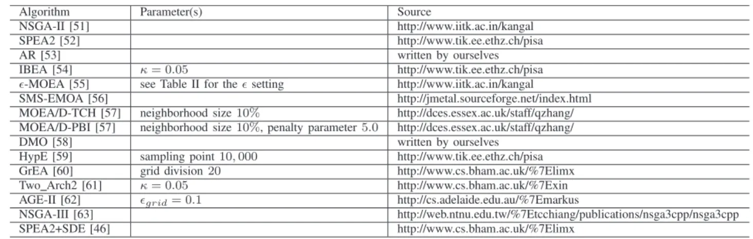
TABLE I

THE PARAMETER SETTING AND THE SOURCE OF THE TESTED ALGORITHMS

Algorithm Parameter(s) Source

NSGA-II [51] http://www.iitk.ac.in/kangal

SPEA2 [52] http://www.tik.ee.ethz.ch/pisa

AR [53] written by ourselves

IBEA [54] κ= 0.05 http://www.tik.ee.ethz.ch/pisa

ǫ-MOEA [55] see Table II for theǫsetting http://www.iitk.ac.in/kangal

SMS-EMOA [56] http://jmetal.sourceforge.net/index.html

MOEA/D-TCH [57] neighborhood size10% http://dces.essex.ac.uk/staff/qzhang/ MOEA/D-PBI [57] neighborhood size10%, penalty parameter5.0 http://dces.essex.ac.uk/staff/qzhang/

DMO [58] written by ourselves

HypE [59] sampling point10,000 http://www.tik.ee.ethz.ch/pisa

GrEA [60] grid division20 http://www.cs.bham.ac.uk/%7Elimx

Two Arch2 [61] κ= 0.05 http://www.cs.bham.ac.uk/%7Exin

AGE-II [62] ǫgrid= 0.1 http://cs.adelaide.edu.au/%7Emarkus

NSGA-III [63] http://web.ntnu.edu.tw/%7Etcchiang/publications/nsga3cpp/nsga3cpp

SPEA2+SDE [46] http://www.cs.bham.ac.uk/%7Elimx

• Diversity Management Operator (DMO)[58]. DMO is

an attempt of using a diversity management operator to adjust the diversity requirement in the selection process of evolutionary many-objective optimization. By comparing the boundary values between the current population and the Pareto front, the diversity maintenance mechanism is controlled (i.e., activated or inactivated).

• Hypervolume Estimation Algorithm (HypE)[59]. As

a representative indicator-based algorithm for many-objective optimization, HypE adopts the Monte Carlo simulation to approximate the exact hypervolume value, thereby significantly reducing the time cost of the HV calculation.

• Grid-based Evolutionary Algorithm (GrEA) [60].

GrEA explores the potential of the use of the grid in many-objective optimization. In GrEA, a set of grid-based criteria are introduced to guide the search towards the optimal front, and a grid-based fitness adjustment strategy to maintain an extensive and uniform distribution among individuals.

• Two-Archive Algorithm 2 (Two Arch2)[61]. As a

bi-population evolutionary algorithm, Two Arch2 considers different selection criteria in the two archive sets, with one set being guided by the indicator Iepsilon+ (from IBEA [54]) and the other by Pareto dominance and a Lp-norm based distance measure, wherepis set to1/m.

• Approximation-Guided Evolutionary Algorithm II (AGE-II) [62]. AGE-II incorporates a formal notion of approximation into an EMO algorithm. To improve the original AGE algorithm [66] suffering from heavy computational cost, AGE-II introduces an adaptive ǫ -dominance approach to balance the convergence speed and runtime. Also, the mating selection strategy is re-designed to emphasize the population diversity.

• Nondominated Sorting Genetic Algorithm III (NSGA-III)[63]. NSGA-III is a recent many-objective algorithm whose framework is based on NSGA-II but with signifi-cant changes in the selection mechanism. Instead of the crowding distance, NSGA-III uses a decomposition-based niching technique to maintain diversity by a set of well-distributed weight vectors.

TABLE II

THE POPULATION SIZE,THEǫSETTING INǫ-MOEA,THE NUMBER OF REFERENCE POINTS/DIRECTIONS(h)ALONG EACH OBJECTIVE IN THE DECOMPOSITION-BASED ALGORITHMSMOEA/D-TCH, MOEA/D-PBI

ANDNSGA-III

Test Instance ǫ h Population Size Group I, 3-Obj. 0.095 14 120 Group II, 3-Obj 0.085 14 120 Group III, 3-Obj 8.000 14 120 Group II, 4-Obj 0.120 7 120 Group III, 4-Obj 10.00 7 120 Group II, 5-Obj 0.135 5 128 Group III, 5-Obj 10.00 5 128 Group I, 10-Obj 0.179 3 220 Group II, 10-Obj 0.179 3 220 Group III, 10-Obj 10.00 3 220

• SPEA2 with Shift-based Density Estimation (SPEA2+SDE) [46]. Shifting individuals’ position before estimating their density, SDE can make Pareto-based algorithms work effectively in many-objective optimization. In contrast to traditional density estimation which only involves individuals’ distribution, SDE covers both the distribution and convergence information of individuals. The Pareto-based algorithm SPEA2 has been demonstrated to be promising when working with SDE.

C. General Experimental Setting

A crossover probabilitypc= 1.0and a mutation probability

pm= 1/n(wherendenotes the number of decision variables)

were used. The operators for crossover and mutation are sim-ulated binary crossover (SBX) and polynomial mutation with both distribution indexes 20. For newly-produced individuals which are located in the constrained areas of the ML-DMP, we simply reproduce them until they are feasible.

The termination criterion of the examined algorithms was 15,000, 30,000 and 60,000 evaluations for Types I, II and III of the ML-DMP instances, respectively. In the decomposition-based algorithms, the population size, which is determined by the number of reference points/directions (h) along each objective, cannot be specified arbitrarily. In the experimental studies, we set h to 14, 7, 5 and 3 for the 3-, 4-, 5- and 10-objective ML-DMP, respectively. In addition, for some of

the tested algorithms, such as NSGA-II and NSGA-III, the population size needs to be divisible by four. In view of these two requirements, we specify the population size (and the archive set) to 120, 120, 128 and 220 for the 3-, 4-, 5- and 10-objective ML-DMPs. In ǫ-MOEA, the size of the archive set is determined by parameterǫ. For a fair comparison, we set ǫ such that the archive set is approximately of the same size as that of the other algorithms. Table I summarizes parameter settings as well as the source of all the algorithms. The setting of these parameters in our experimental studies either follows the suggestion in their original papers or has been found to enable the algorithm to perform better on the ML-DMP.

IV. EXPERIMENTALRESULTS

In this section, we examine the search behavior of the 15 EMO algorithms by demonstrating their solution sets in the two-dimensional decision space for the three types of ML-DMP instances described in the previous section. Each algorithm was executed 10 independent runs, from which we displayed the best solution set (determined by the IGD indicator [28]) of one run. For a quantitative understanding, the GD [67] and IGD results of the best solution set were also included in the figures. GD and IGD are two popular performance indicators which assess a solution set’s conver-gence and comprehensive performance (i.e., both converconver-gence and diversity), respectively. To calculate GD, we considered the average Euclidean distance of the solutions to the optimal polygon. That is, if a solution is inside the optimal polygon the distance is zero; otherwise, it is the distance from the solution to its closest edge of the polygon. For IGD, we randomly generated 50,000 points inside the optimal polygon and then calculated the average Euclidean distance from these points to their closest solution in the considered solution set.

In addition, to examine the stability of the algorithms in terms of convergence and diversity individually, we provide two number indexes I1 and I2, with I1 being the number of runs (out of all 10 runs) in which the final solutions obtained by the tested algorithm converge into (or are very close to) the optimal polygon and I2 being the number of runs in which the solutions have a good coverage over the optimal polygon. These two indexes are determined by GD and IGD, respectively.

A. Type I ML-DMP

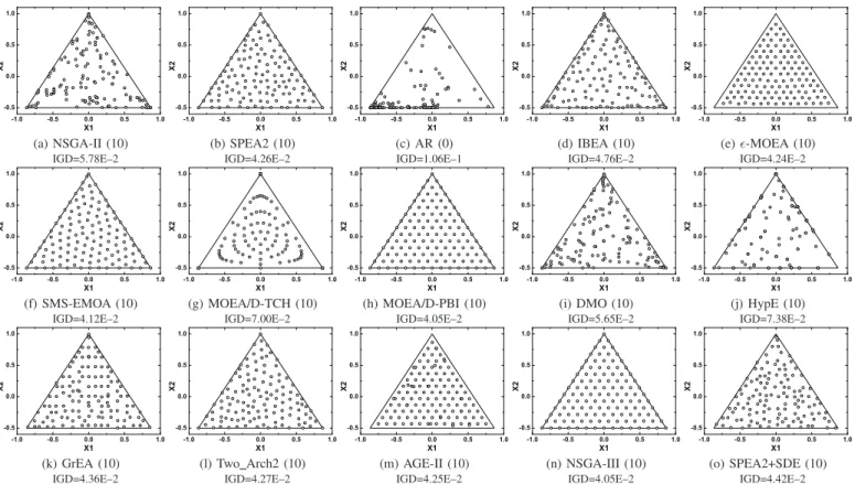
Fig. 5 shows the best one-run solution sets obtained by the 15 algorithms on the tri-objective Type I ML-DMP instance where the search space is precisely the optimal triangle. This allows an independent examination of the algorithms’ performance in maintaining diversity. As can be seen in the figure, the solutions of all the algorithms except AR are widely distributed over the triangle, which verifies their ability in di-versifying the population on the tri-objective problem. Among these algorithms, however, some fail to maintain the unifor-mity of distribution, leading to the solutions crowded (or even overlapping) in some areas but sparse in some others. Such algorithms includes NSGA-II, DMO, HypE, and MOEA/D-TCH; the last one, interestingly, has a regularly-distributed

solution set. In contrast, the solutions obtained by ǫ-MOEA and AGE-II have an excellent uniformity, but cannot cover the boundary of the triangle. SPEA2, IBEA, GrEA, Two Arch2 and SPEA2+SDE are the algorithms which achieve a good bal-ance between uniformity and extensity. In addition, three well-known algorithms, SMS-EMOA, MOEA/D-PBI and NSGA-III, tend to have a perfect performance on this problem, with their solutions being highly uniform over the whole triangle.

The above observations show that most of the tested EMO algorithms are able to effectively maintain solutions’ diversity on the tri-objective instance. So, how do they perform when more objectives are involved? Fig. 6 gives the results of the best solution sets of the 15 algorithms on the 10-objective Type I instance. We here do not show the results on 4- and 5-objective instances since the algorithms perform very similarly on all the Type I instances with more than three objectives. As shown in the figure, most of the algorithms have the similar pattern as in the tri-objective instance. This means that their ability of maintaining diversity does not degrade with the increase of the number of objectives. That is, if there are sufficient well-converged solutions being produced during the evolutionary process, these algorithms can diversify them well even in the high-dimensional space.

Nevertheless, there do exist some algorithms which scale up badly with the number of objectives. They include ǫ -MOEA, SMS-EMOA, MOEA/D-TCH, MOEA/D-PBI, HypE and NSGA-III. It is worth mentioning that all of these algo-rithms do not use directly density-based methods in diversity maintenance.ǫ-MOEA maintains the population diversity by the ǫ dominance, SMS-EMOA and HypE rely on the HV indicator, and MOEA/D-TCH, MOEA/D-PBI and NSGA-III use the decomposition-based strategy. The failure ofǫ-MOEA in obtaining a uniformly-distributed solution set suggests the difficulty that the ǫdominance faces in the high-dimensional space. One possible explanation of SMS-EMOA and HypE’s underperformance on the 10-objective instance is that an approximate estimation of the HV contribution may affect the performance of the algorithms. In addition, it is not surprising that the three decomposition-based algorithms cannot maintain solutions’ diversity on this instance since the ML-DMP with more than three objectives has a degenerate Pareto front (i.e., the dimensionality of the Pareto front is less than the number of objectives), on which decomposition-based algorithms com-monly struggle [31], [63]. Finally, an interesting observation is that AR which does not use any diversity maintenance scheme during the evolutionary process performs better than some of the other algorithms (such as MOEA/D-TCH and HypE). This indicates that random selection could even pick out more diversified individuals than some decomposition-based or indicator-decomposition-based selection in high-dimensional ML-DMP problems.

B. Type II ML-DMP

The search space of the Type II ML-DMP problem is [−100,100]2_{, significantly larger than the optimal region (<} [−1,1]2_{), thus providing a challenge for EMO algorithms to} achieve a balance between convergence and diversity. Fig. 7

-1.0 -0.5 0.0 0.5 1.0 -0.5 0.0 0.5 1.0 X 2 X1 -1.0 -0.5 0.0 0.5 1.0 -0.5 0.0 0.5 1.0 X 2 X1 -1.0 -0.5 0.0 0.5 1.0 -0.5 0.0 0.5 1.0 X 2 X1 -1.0 -0.5 0.0 0.5 1.0 -0.5 0.0 0.5 1.0 X 2 X1 -1.0 -0.5 0.0 0.5 1.0 -0.5 0.0 0.5 1.0 X1 X 2

(a) NSGA-II (10) (b) SPEA2 (10) (c) AR (0) (d) IBEA (10) (e)ǫ-MOEA (10)

IGD=5.78E–2 IGD=4.26E–2 IGD=1.06E–1 IGD=4.76E–2 IGD=4.24E–2

-1.0 -0.5 0.0 0.5 1.0 -0.5 0.0 0.5 1.0 X 2 X1 -1.0 -0.5 0.0 0.5 1.0 -0.5 0.0 0.5 1.0 X 2 X1 -1.0 -0.5 0.0 0.5 1.0 -0.5 0.0 0.5 1.0 X1 X 2 -1.0 -0.5 0.0 0.5 1.0 -0.5 0.0 0.5 1.0 X 2 X1 -1.0 -0.5 0.0 0.5 1.0 -0.5 0.0 0.5 1.0 X 2 X1

(f) SMS-EMOA (10) (g) MOEA/D-TCH (10) (h) MOEA/D-PBI (10) (i) DMO (10) (j) HypE (10)

IGD=4.12E–2 IGD=7.00E–2 IGD=4.05E–2 IGD=5.65E–2 IGD=7.38E–2

-1.0 -0.5 0.0 0.5 1.0 -0.5 0.0 0.5 1.0 X 2 X1 -1.0 -0.5 0.0 0.5 1.0 -0.5 0.0 0.5 1.0 X 2 X1 -1.0 -0.5 0.0 0.5 1.0 -0.5 0.0 0.5 1.0 X 2 X1 -1.0 -0.5 0.0 0.5 1.0 -0.5 0.0 0.5 1.0 X 2 X1 -1.0 -0.5 0.0 0.5 1.0 -0.5 0.0 0.5 1.0 X 2 X1

(k) GrEA (10) (l) Two Arch2 (10) (m) AGE-II (10) (n) NSGA-III (10) (o) SPEA2+SDE (10)

IGD=4.36E–2 IGD=4.27E–2 IGD=4.25E–2 IGD=4.05E–2 IGD=4.42E–2

Fig. 5. The best solution set of the 15 algorithms on a tri-objective ML-DMP instance where the search space is precisely the optimal polygon, and its corresponding IGD result. The associated index of the algorithm represents the number of runs (out of all 10 runs) in which the obtained solutions have a good coverage over the optimal polygon.

-1.0 -0.5 0.0 0.5 1.0 -1.0 -0.5 0.0 0.5 1.0 X 2 X1 -1.0 -0.5 0.0 0.5 1.0 -1.0 -0.5 0.0 0.5 1.0 X 2 X1 -1.0 -0.5 0.0 0.5 1.0 -1.0 -0.5 0.0 0.5 1.0 X 2 X1 -1.0 -0.5 0.0 0.5 1.0 -1.0 -0.5 0.0 0.5 1.0 X 2 X1 -1.0 -0.5 0.0 0.5 1.0 -1.0 -0.5 0.0 0.5 1.0 X 2 X1

(a) NSGA-II (10) (b) SPEA2 (10) (c) AR (9) (d) IBEA (10) (e)ǫ-MOEA (10)

IGD=6.01E–2 IGD=4.65E–2 IGD=8.11E–2 IGD=4.98E–2 IGD=5.40E–2

-1.0 -0.5 0.0 0.5 1.0 -1.0 -0.5 0.0 0.5 1.0 X 2 X1 -1.0 -0.5 0.0 0.5 1.0 -1.0 -0.5 0.0 0.5 1.0 X 2 X1 -1.0 -0.5 0.0 0.5 1.0 -1.0 -0.5 0.0 0.5 1.0 X 2 X1 -1.0 -0.5 0.0 0.5 1.0 -1.0 -0.5 0.0 0.5 1.0 X1 X 2 -1.0 -0.5 0.0 0.5 1.0 -1.0 -0.5 0.0 0.5 1.0 X1 X 2

(f) SMS-EMOA (10) (g) MOEA/D-TCH (0) (h) MOEA/D-PBI (0) (i) DMO (10) (j) HypE (0)

IGD=6.18E–2 IGD=1.30E–1 IGD=1.51E–1 IGD=6.00E–2 IGD=2.62E–1

-1.0 -0.5 0.0 0.5 1.0 -1.0 -0.5 0.0 0.5 1.0 X1 X 2 -1.0 -0.5 0.0 0.5 1.0 -1.0 -0.5 0.0 0.5 1.0 X1 X 2 -1.0 -0.5 0.0 0.5 1.0 -1.0 -0.5 0.0 0.5 1.0 X 2 X1 -1.0 -0.5 0.0 0.5 1.0 -1.0 -0.5 0.0 0.5 1.0 X 2 X1 -1.0 -0.5 0.0 0.5 1.0 -1.0 -0.5 0.0 0.5 1.0 X 2 X1

(k) GrEA (10) (l) Two Arch2 (10) (m) AGE-II (10) (n) NSGA-III (0) (o) SPEA2+SDE (10)

IGD=4.87E–2 IGD=4.78E–2 IGD=4.69E–2 IGD=9.03E–2 IGD=4.84E–2

Fig. 6. The best solution set of the 15 algorithms on a ten-objective ML-DMP instance where the search space is precisely the optimal polygon, and its corresponding IGD result. The associated index of the algorithm represents the number of runs (out of all 10 runs) in which the obtained solutions have a good coverage over the optimal polygon.

-1.0 -0.5 0.0 0.5 1.0 -0.5 0.0 0.5 1.0 X 2 X1 -1.0 -0.5 0.0 0.5 1.0 -0.5 0.0 0.5 1.0 X 2 X1 -1.0 -0.5 0.0 0.5 1.0 -0.5 0.0 0.5 1.0 X 2 X1 -1.0 -0.5 0.0 0.5 1.0 -0.5 0.0 0.5 1.0 X 2 X1 -1.0 -0.5 0.0 0.5 1.0 -0.5 0.0 0.5 1.0 X1 X 2

(a) NSGA-II (10, 10) (b) SPEA2 (10, 10) (c) AR (10, 0) (d) IBEA (10, 0) (e)ǫ-MOEA (10, 10)

GD=3.10E–3, IGD=6.38E–2 GD=1.25E–3, IGD=4.28E–2 GD=2.65E–3, IGD=1.16E–1 GD=2.24E–4, IGD=1.05E–1 GD=0.00E+0, IGD=4.32E–2

-1.0 -0.5 0.0 0.5 1.0 -0.5 0.0 0.5 1.0 X 2 X1 -1.0 -0.5 0.0 0.5 1.0 -0.5 0.0 0.5 1.0 X 2 X1 -1.0 -0.5 0.0 0.5 1.0 -0.5 0.0 0.5 1.0 X1 X 2 -1.0 -0.5 0.0 0.5 1.0 -0.5 0.0 0.5 1.0 X 2 X1 -1.0 -0.5 0.0 0.5 1.0 -0.5 0.0 0.5 1.0 X 2 X1

(f) SMS-EMOA (10, 10) (g) MOEA/D-TCH (10, 10) (h) MOEA/D-PBI (10, 10) (i) DMO (9, 10) (j) HypE (10, 10)

GD=2.98E–5, IGD=4.16E–2 GD=2.51E–5, IGD=6.45E–2 GD=4.01E–5, IGD=4.17E–2 GD=2.43E–3, IGD=6.17E–2 GD=1.37E–4, IGD=8.09E–2

-1.0 -0.5 0.0 0.5 1.0 -0.5 0.0 0.5 1.0 X 2 X1 -1.0 -0.5 0.0 0.5 1.0 -0.5 0.0 0.5 1.0 X1 X 2 -1.0 -0.5 0.0 0.5 1.0 -0.5 0.0 0.5 1.0 X 2 X1 -1.0 -0.5 0.0 0.5 1.0 -0.5 0.0 0.5 1.0 X 2 X1 -1.0 -0.5 0.0 0.5 1.0 -0.5 0.0 0.5 1.0 X 2 X1

(k) GrEA (10, 7) (l) Two Arch2 (10, 10) (m) AGE-II (10, 10) (n) NSGA-III (10, 10) (o) SPEA2+SDE (10, 10)

GD=5.07E–6, IGD=4.53E–2 GD=1.89E–3, IGD=4.64E–2 GD=0.00E+0, IGD=4.27E–2 GD=2.88E–4, IGD=4.06E–2 GD=1.96E–4, IGD=4.37E–2

Fig. 7. The best solution set of the 15 algorithms on a tri-objective ML-DMP instance where the search space is[−100,100]

2

, and its corresponding GD and IGD results. The associated indexes (I1,I2) of the algorithm respectively represent the number of runs (out of all 10 runs) in which all obtained solutions converge into (or are close to) the optimal polygon and the number of runs in which the obtained solutions have a good coverage over the optimal polygon.

-100 -50 0 50 100 -100 -50 0 50 100 X 2 X1 -100 -50 0 50 100 -100 -50 0 50 100 X 2 X1 -20 -10 0 10 20 -20 -10 0 10 20 X 2 X1 -1.0 -0.5 0.0 0.5 1.0 -1.0 -0.5 0.0 0.5 1.0 X 2 X1 -1.0 -0.5 0.0 0.5 1.0 -1.0 -0.5 0.0 0.5 1.0 X1 X 2

(a) NSGA-II (0, 0) (b) SPEA2 (0, 0) (c) AR (0, 0) (d) IBEA (10, 0) (e)ǫ-MOEA (10, 10)

GD=4.20E+1, IGD=5.45E–1 GD=3.63E+1, IGD=4.92E–1 GD=3.81E+0, IGD=1.42E–1 GD=1.70E–4, IGD=2.72E–1 GD=0.00E+0, IGD=5.32E–2

-1.0 -0.5 0.0 0.5 1.0 -1.0 -0.5 0.0 0.5 1.0 X 2 X1 -40 -20 0 20 40 -40 -20 0 20 40 X 2 X1 -1.5 -1.0 -0.5 0.0 0.5 1.0 1.5 -1.5 -1.0 -0.5 0.0 0.5 1.0 1.5 X1 X 2 -40 -20 0 20 40 -40 -20 0 20 40 X 2 X1 -1.0 -0.5 0.0 0.5 1.0 -1.0 -0.5 0.0 0.5 1.0 X 2 X1

(f) SMS-EMOA (10, 10) (g) MOEA/D-TCH (0, 0) (h) MOEA/D-PBI (0, 10) (i) DMO (0, 0) (j) HypE (10, 10)

GD=3.21E–5, IGD=5.78E–2 GD=8.03E–1, IGD=9.63E–2 GD=6.71E–2, IGD=7.66E–2 GD=7.60E+0, IGD=1.50E–1 GD=2.83E–4, IGD=8.44E–2

-3 -2 -1 0 1 2 3 -3 -2 -1 0 1 2 3 X 2 X1 -40 -20 0 20 40 -40 -20 0 20 40 X 2 X1 -1.0 -0.5 0.0 0.5 1.0 -1.0 -0.5 0.0 0.5 1.0 X 2 X1 -10 -5 0 5 10 -10 -5 0 5 10 X 2 X1 -1.0 -0.5 0.0 0.5 1.0 -1.0 -0.5 0.0 0.5 1.0 X 2 X1

(k) GrEA (5, 0) (l) Two Arch2 (0, 0) (m) AGE-II (10, 10) (n) NSGA-III (0, 0) (o) SPEA2+SDE (10, 10)

GD=2.72E–2, IGD=1.56E–1 GD=1.53E+1, IGD=2.11E–1 GD=0.00E+0, IGD=5.36E–2 GD=4.88E+0, IGD=1.23E–1 GD=0.00E+0, IGD=5.34E–2

Fig. 8. The best solution set of the 15 algorithms on a four-objective ML-DMP instance where the search space is[−100,100]

2

, and its corresponding GD and IGD results. The associated indexes (I1,I2) of the algorithm respectively represent the number of runs (out of all 10 runs) in which all obtained solutions converge into (or are close to) the optimal polygon and the number of runs in which the obtained solutions have a good coverage over the optimal polygon.

P2 P1

A1 A2

A4 A3

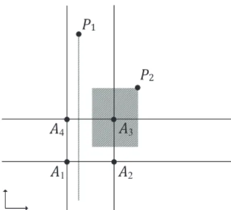
Fig. 9. An illustration of the difficulty for EMO algorithms to converge on the four-objective ML-DMP problem. whereA1,A2,A3andA4are the four vertexes of the optimal polygon. The shadows are the regions that dominate

P1andP2, respectively.

shows the best one-run solution sets obtained by the 15 algorithms on the tri-objective instance. As shown, all the algorithms have a good convergence, with their individuals inside (or very close to) the optimal triangle. Also, the solution sets obtained by most algorithms are distributed similarly as on the Type I ML-DMP. One exception is IBEA, which performs significantly worse than on the Type I instance since many of its solutions are overlapping. This indicates that the measure of IBEA’s indicator prefers overlapping solutions to poorly-converged ones.

The above results show the ability of the examined al-gorithms in balancing convergence and diversity on the tri-objective ML-DMP. Then, how do they perform on the prob-lem with more objectives? Fig. 8 shows the solution sets obtained by the 15 algorithms on the four-objective Type II ML-DMP. As shown, only five algorithms, ǫ-MOEA, SMS-EMOA, AGE-II, SPEA2+SDE, and HypE, perform well on this problem, from whichǫ-MOEA has an excellent uniformity and SMS-EMOA, AGE-II and SPEA2+SDE have a good bal-ance between uniformity and extensity. Most of the remaining algorithms are unable to guide their population to converge into the optimal rectangle, with their solution sets typically distributed in the form of a cross.

Fig. 9 gives an illustration to explain why this happens. P1 and P2 are two solutions for a four-objective ML-DMP problem with four vertexes A1, A2, A3 and A4. P1 resides between two parallel target lines ←−−→A1A4 and ←−−→A2A3, and P2 in the right upper area to the optimal square. As seen, the region that Pareto dominatesP1is a line segment, far smaller than that dominatingP2, althoughP1is farther to the optimal polygon than P2. In fact, any solution (outside the optimal polygon) located between a pair of parallel target lines is dominated by only a line segment parallel to these two lines; an improvement of its distance to the one line will lead to the degradation to the other. This property poses a big challenge not only for the algorithms who use Pareto dominance as the main selection criterion, such as NSGA-II, SPEA2, DMO, Two Arch2 and NSGA-INSGA-II, but also for some other modern algorithms, such as MOEA/D-TCH and GrEA. The solutions obtained by these algorithms can easily

be distributed crisscross in the space.

Fig. 10 shows the solution sets obtained by the 15 algo-rithms on the five-objective instance. Similar to the situation on the four-objective instance, the Pareto-based EMO algorithms struggle to converge. This is because solutions in some regions (i.e., the boundary of the constrained polygons) are only dominated by one point in the pentagon. One difference from the four-objective situation is that all the solutions obtained by MOEA/D-PBI and GrEA can converge into the optimal region. This indicates that the difficulty of the ML-DMP problem does not certainly increase with the number of objectives.

When the considered objective dimensionality of the ML-DMP is 10, both parallel target lines and constrained areas are involved in the problem. This naturally leads to bigger challenges for EMO algorithms to balance the convergence and diversity. As can be seen in Fig. 11, only three algorithms, ǫ-MOEA, AGE-II and SPEA2+SDE, work well on the 10-objective instance. The solution sets of IBEA, MOEA/D-PBI and HypE can converge into the optimal region but fail to cover the whole polygon.

C. Type III ML-DMP

Type III ML-DMP hugely extends the problem’s search space ([−1010_,1010_{]) to test the algorithms’ ability of leading} solutions to converge towards the Pareto optimal region. Fig. 12 shows the best one-run solution sets obtained by the 15 algorithms on the tri-objective instance. An interesting ob-servation is that different decomposition-based and indicator-based algorithms behave rather differently, such as IBEA vs SMS-EMOA and HypE, and MOEA/D vs NSGA-III. One explanation for this is that the Pareto dominance criterion can effectively guide the population into the optimal region – the decomposition-based and indicator-based algorithms which use Pareto dominance as the primary selection criterion (i.e., SMS-EMOA, HypE and NSGA-III) perform much better than those not using the Pareto dominance criterion (i.e., IBEA, MOEA/D-TCH and MOEA/D-PBI). This has also been proven by the fact that some classic Pareto-based algorithms work well on this problem, such as NSGA-II and SPEA2. In addition, note that only one solution is obtained byǫ-MOEA. In fact, no matter how the ǫ value of the algorithm is set, there is always a sole solution left in the final archive set when the problem’s search space becomes huge. This applies to all the Type III ML-DMP instances with any number of objectives. Finally, it is worth mentioning that there is none of the tested algorithms able to obtain a stable performance in terms of both convergence and diversity, as shown by the two indexes I1 and I2 in the figure. This indicates that the proposed problem poses great challenges for EMO algorithms even in the three-dimensional space.

Consider the 4- and 5-objective instances shown in Fig. 13 and Fig. 14, respectively. Only AGE-II and SPEA2+SDE are able to find a well-converged, well-distributed solution set on both instances. HypE performs fairly well on the 4-objective instance, and SMS-EMOA occasionally converges for the objective instance. Interesting observations regarding the 5-objective results are from SPEA2 and Two Arch2 which

-6 -3 0 3 6 -6 -3 0 3 6 X 2 X1 -6 -3 0 3 6 -6 -3 0 3 6 X 2 X1 -4 -2 0 2 4 -4 -2 0 2 4 X 2 X1 -1.0 -0.5 0.0 0.5 1.0 -1.0 -0.5 0.0 0.5 1.0 X 2 X1 -1.0 -0.5 0.0 0.5 1.0 -1.0 -0.5 0.0 0.5 1.0 X1 X 2

(a) NSGA-II (0, 0) (b) SPEA2 (0, 0) (c) AR (0, 0) (d) IBEA (10, 0) (e)ǫ-MOEA (10, 10)

GD=2.48E+0, IGD=2.40E–1 GD=1.59E+0, IGD=1.01E–1 GD=1.16E–1, IGD=1.12E–1 GD=2.73E–4, IGD=4.36E–1 GD=0.00E+0, IGD=5.78E–2

-1.0 -0.5 0.0 0.5 1.0 -1.0 -0.5 0.0 0.5 1.0 X 2 X1 -3 0 3 6 9 -6 -4 -2 0 2 4 X 2 X1 -1.0 -0.5 0.0 0.5 1.0 -1.0 -0.5 0.0 0.5 1.0 X1 X 2 -3 -2 -1 0 1 2 3 -3 -2 -1 0 1 2 3 X 2 X1 -1.0 -0.5 0.0 0.5 1.0 -1.0 -0.5 0.0 0.5 1.0 X 2 X1

(f) SMS-EMOA (10, 10) (g) MOEA/D-TCH (0, 10) (h) MOEA/D-PBI (10, 10) (i) DMO (0, 0) (j) HypE (10, 10)

GD=1.81E–4, IGD=6.97E–2 GD=2.50E–1, IGD=7.76E–2 GD=0.00E+0, IGD=7.33E–2 GD=2.76E–1, IGD=1.15E–1 GD=0.00E+0, IGD=8.57E–2

-1.0 -0.5 0.0 0.5 1.0 -1.0 -0.5 0.0 0.5 1.0 X 2 X1 -2 0 2 4 -4 -2 0 2 X 2 X1 -1.0 -0.5 0.0 0.5 1.0 -1.0 -0.5 0.0 0.5 1.0 X 2 X1 -4 -2 0 2 4 -4 -2 0 2 4 X 2 X1 -1.0 -0.5 0.0 0.5 1.0 -1.0 -0.5 0.0 0.5 1.0 X 2 X1

(k) GrEA (9, 9) (l) Two Arch2 (0, 7) (m) AGE-II (10, 10) (n) NSGA-III (0, 0) (o) SPEA2+SDE (9, 10)

GD=0.00E+0, IGD=6.53E–2 GD=6.30E–1, IGD=7.77E–2 GD=0.00E+0, IGD=5.77E–2 GD=6.23E–1, IGD=1.08E–1 GD=0.00E+0, IGD=5.80E–2

Fig. 10. The best solution set of the 15 algorithms on a five-objective ML-DMP instance where the search space is[−100,100]

2

, and its corresponding GD and IGD results. The associated indexes (I1,I2) of the algorithm respectively represent the number of runs (out of all 10 runs) in which all obtained solutions converge into (or are close to) the optimal polygon and the number of runs (out of all 10 runs) in which the obtained solutions have a good coverage over the optimal polygon.

-100 -50 0 50 100 -100 -50 0 50 100 X 2 X1 -100 -50 0 50 100 -100 -50 0 50 100 X 2 X1 -60 -30 0 30 60 -60 -30 0 30 60 X 2 X1 -1.0 -0.5 0.0 0.5 1.0 -1.0 -0.5 0.0 0.5 1.0 X 2 X1 -1.0 -0.5 0.0 0.5 1.0 -1.0 -0.5 0.0 0.5 1.0 X1 X 2

(a) NSGA-II (0, 0) (b) SPEA2 (0, 0) (c) AR (0, 0) (d) IBEA (10, 0) (e)ǫ-MOEA (10, 10)

GD=7.03E+1, IGD=1.11E+0 GD=5.62E+1, IGD=8.44E–1 GD=6.21E+0, IGD=1.19E–1 GD=0.00E+0, IGD=3.70E–1 GD=0.00E+0, IGD=5.31E–2

-40 -20 0 20 40 -30 -20 -10 0 10 20 30 X 2 X1 -10 -5 0 5 10 -2 -1 0 1 2 X 2 X1 -1.0 -0.5 0.0 0.5 1.0 -1.0 -0.5 0.0 0.5 1.0 X1 X 2 -40 -20 0 20 40 -40 -20 0 20 40 X 2 X1 -1.0 -0.5 0.0 0.5 1.0 -1.0 -0.5 0.0 0.5 1.0 X 2 X1

(f) SMS-EMOA (0, 0) (g) MOEA/D-TCH (0, 0) (h) MOEA/D-PBI (10, 0) (i) DMO (0, 0) (j) HypE (10, 0)

GD=5.75E+0, IGD=1.02E–1 GD=1.86E–1, IGD=1.39E–1 GD=0.00E+0, IGD=1.54E–1 GD=1.05E+1, IGD=4.97E–1 GD=0.00E+0, IGD=2.56E–1

-10 -5 0 5 10 -10 -5 0 5 10 X 2 X1 -100 -50 0 50 100 -100 -50 0 50 100 X 2 X1 -1.0 -0.5 0.0 0.5 1.0 -1.0 -0.5 0.0 0.5 1.0 X 2 X1 -30 -20 -10 0 10 20 30 -30 -20 -10 0 10 20 30 X 2 X1 -1.0 -0.5 0.0 0.5 1.0 -1.0 -0.5 0.0 0.5 1.0 X 2 X1

(k) GrEA (0, 0) (l) Two Arch2 (0, 0) (m) AGE-II (10, 10) (n) NSGA-III (0, 0) (o) SPEA2+SDE (10, 10)

GD=2.35E+0, IGD=1.44E–1 GD=5.24E+1, IGD=5.06E–1 GD=0.00E+0, IGD=4.76E–2 GD=6.30E+0, IGD=1.55E–1 GD=0.00E+0, IGD=4.79E–2

Fig. 11. The best solution set of the 15 algorithms on a ten-objective ML-DMP instance where the search space is[−100,100]

2

, and its corresponding GD and IGD results. The associated indexes (I1,I2) of the algorithm respectively represent the number of runs (out of all 10 runs) in which all obtained solutions converge into (or are close to) the optimal polygon and the number of runs in which the obtained solutions have a good coverage over the optimal polygon.

-1.0 -0.5 0.0 0.5 1.0 -0.5 0.0 0.5 1.0 X 2 X1 -1.0 -0.5 0.0 0.5 1.0 -0.5 0.0 0.5 1.0 X 2 X1 -3 0 3 6 9 12 -1.0 -0.5 0.0 0.5 1.0 X 2 X1 -60 -50 -40 -30 -20 -10 0 10 -100 -50 0 50 100 X 2 X1 -1.0 -0.5 0.0 0.5 1.0 -0.5 0.0 0.5 1.0 X 2 X1

(a) NSGA-II (2, 4) (b) SPEA2 (2, 3) (c) AR (0, 0) (d) IBEA (0, 0) (e)ǫ-MOEA (7, 0)

GD=6.12E–3, IGD=7.08E–2 GD=1.46E–3, IGD=4.36E–2 GD=4.31E+1, IGD=4.72E+2 GD=2.18E+1, IGD=1.31E+2 GD=0.00E+0, IGD=5.06E–1

-1.0 -0.5 0.0 0.5 1.0 -0.5 0.0 0.5 1.0 X 2 X1 -120 -100 -80 -60 -40 -20 0 0 20 40 60 X 2 X1 -2000 -1500 -1000 -500 0 0 500 1000 1500 X1 X 2 -1.0 -0.5 0.0 0.5 1.0 -0.5 0.0 0.5 1.0 X 2 X1 -1.0 -0.5 0.0 0.5 1.0 -0.5 0.0 0.5 1.0 X 2 X1

(f) SMS-EMOA (3, 3) (g) MOEA/D-TCH (0, 0) (h) MOEA/D-PBI (0, 0) (i) DMO (5, 2) (j) HypE (4, 2)

GD=8.15E–5, IGD=4.31E–2 GD=8.40E+1, IGD=2.99E+2 GD=7.19E+2, IGD=1.99E+3 GD=4.01E–4, IGD=7.60E–2 GD=7.19E–4, IGD=8.75E–2

-1.0 -0.5 0.0 0.5 1.0 -0.5 0.0 0.5 1.0 X1 X 2 -1.0 -0.5 0.0 0.5 1.0 -0.5 0.0 0.5 1.0 X 2 X1 -1.0 -0.5 0.0 0.5 1.0 -0.5 0.0 0.5 1.0 X 2 X1 -1.0 -0.5 0.0 0.5 1.0 -0.5 0.0 0.5 1.0 X 2 X1 -1.0 -0.5 0.0 0.5 1.0 -0.5 0.0 0.5 1.0 X 2 X1

(k) GrEA (4, 0) (l) Two Arch2 (5, 5) (m) AGE-II (4, 1) (n) NSGA-III (4, 2) (o) SPEA2+SDE (8, 5)

GD=3.61E–4, IGD=1.60E–1 GD=3.50E–3, IGD=5.05E–2 GD=0.00E+0, IGD=5.36E–2 GD=3.70E–4, IGD=4.25E–2 GD=2.33E–4, IGD=4.98E–2

Fig. 12. The best solution set of the 15 algorithms on a tri-objective ML-DMP instance where the search space is[−10

10_, 1010

]2

, and its corresponding GD and IGD results. The associated indexes (I1,I2) of the algorithm respectively represent the number of runs (out of all 10 runs) in which all obtained solutions converge into (or are close to) the optimal polygon and the number of runs in which the obtained solutions have a good coverage over the optimal polygon.

sometimes have a good coverage over the optimal pentagon, but cannot lead all of their solutions into the optimal region.

The Type III 10-objective ML-DMP is the hardest problem that we tested in this experimental study. As can be seen in Fig. 15, only SPEA2+SDE can obtain a good convergence and diversity on nearly half of the 10 runs. Among the other algorithms, IBEA andǫ-MOEA can occasionally converge, but their solutions concentrate in either several boundary points or the central point of the polygon.

D. Summary

On the basis of the investigation on the three types of ten ML-DMP instances, the following observations of the 15 EMO algorithms can be made:

• Despite failing on the ML-DMP with two parallel target

lines, the conventional Pareto-based algorithms NSGA-II and SPEA2 have shown their advantage on the low-dimensional instances. They clearly outperform some of the decomposition-based or indicator-based algorithms (e.g., MOEA/D-TCH, MOEA/D-PBI and IBEA) on the 3-objective Type III ML-DMP.

• Due to the lack of diversity maintenance, AR is the

algorithm with poor performance on all the instances but the 10-objective Type I, where AR is superior to MOEA/D-TCH and HypE in terms of diversity.

• The performance of IBEA varies, with its solutions

dis-tributed well on the Type I instances, concentrating into

the boundaries of the polygon on the Type II instances, and being generally far from the optimal region on the Type III instances.

• ǫ-MOEA performs well on all the Type I and II instances,

but cannot diversify its solutions on the Type III instances. An interesting observation is that ǫ-MOEA struggles to maintain the uniformity on the 10-objective ML-DMP. This is in contrary to some previous studies [19], [68], where the ǫ dominance has been demonstrated to work well in this respect in the high-dimensional space.

• SMS-EMOA performs excellently on many relatively

easy ML-DMP instances (e.g., on all the 3-objective in-stances). However, when the number of objectives reaches ten, SMS-EMOA fails to provide a good balance between convergence and diversity.

• MOEA/D-TCH struggles to maintain the uniformity of

the solutions over the optimal polygon. This, as explained in [63], is because in the Tchebycheff metric a uniform set of weight vectors may not lead to a uniformly-distributed solutions. In addition, in most cases MOEA/D-TCH cannot guide all of its solutions to converge into the optimal region, although the algorithm performs signifi-cantly better than most of the tested algorithms in terms of convergence on the Type III instances.

• The performance of MOEA/D-PBI has a sharp contrast

on different instances. It performs perfectly on the 3-objective Type I and II ML-DMPs, but cannot maintain