DDoS: DeepDefence and Machine Learning for identifying attacks

QATAR UNIVERSITY

COLLEGE OF ENGINEERING

DDoS: DEEPDEFENCE AND MACHINE LEARNING FOR IDENTIFYING

ATTACKS

BY

AKHILESH BHATI

A Thesis Submitted to the College of Engineering

in Partial Fulfillment of the Requirements for the Degree of Master of Science in Computing

June 2020

COMMITTEE PAGE

The members of the Committee approve the Thesis of Akhilesh Bhati defended on 28-April-2020

___________________________________ Dr. Abdelaziz Bouras Thesis/Dissertation Supervisor

___________________________________ Dr. Uvais Ahmed Qidwai

Co-Supervisor

___________________________________ Dr. Osama Halabi Committee Member

___________________________________ Dr. Radhouane Ben Hamadou

Committee Member ___________________________________ Dr. Ibrahim Khalil Committee Member

Approved:

ABSTRACT

BHATI, AKHILESH, Masters: June 2020, Masters of Science in Computing Title: DDoS: DeepDefence and Machine Learning for identifying attacks Supervisor of Thesis: Dr. Abdelaziz Bouras

Distributed Denial of Service (DDoS) attacks are very common type of computer attack in the world of internet today. Automatically detecting such type of DDoS attack packets & dropping them before passing through the network is the best prevention method. Conventional solution only monitors and provide the feedforward solution instead of the feedback machine-based learning. A Design of Deep neural network has been suggested in this work and developments have been made on proactive detection of attacks. In this approach, high level features are extracted for representation and inference of the dataset. Experiment has been conducted based on the ISCX dataset published in year 2017,2018 and CICDDoS2019 and program has been developed in Matlab R17b, utilizing Wireshark for features extraction from the datasets.

Network Intrusion attacks on critical oil and gas industrial installation become common nowadays, which in turn bring down the giant industrial sites to standstill and suffer financial impacts. This has made the production companies to started investing millions of dollars revenue to protect their critical infrastructure with such attacks with the active and passive solutions available. Our thesis constitutes a contribution to such domain, focusing mainly on security of industrial network, impersonation and attacking with DDoS.

iv DEDICATION

I dedicate this work to my thesis Supervisor Dr. Abdelaziz Bouras and my children Abhishek and Aakanksha.

ACKNOWLEDGMENTS

Technical and moral support provided by my supervisor Dr. Abdelaziz Bouras, I cannot forget, without which it was near to impossible for me to achieve this work.

I acknowledge the support of Dr. Uvais Ahmed Qidwai for guiding me in troubleshooting the various problems faced during the simulation of the experiment.

vi

TABLE OF CONTENT

1.1. Distributed Denial of Service attack: ... 1

1.2. Problem Statement ... 2

1.3. Research Questions ... 2

1.4. Research Objectives ... 2

1.5. Thesis Outline ... 3

CHAPTER 2: Literature Review ... 4

2.1. DDoS Research and description ... 4

2.2. Classification of DDoS ... 6

2.2.1. Impact Size: ... 6

2.2.2. Degrading Network: ... 6

2.3. Based on network Vulnerability ... 6

2.3.1. Flood Attack: ... 6

2.3.2. Amplification Attack using DNS: ... 7

2.3.4. Malformed Server Packet attack ... 7

2.4. Countermeasure ... 8

2.4.1. Ingres Filtering: ... 8

2.4.2. D-Ward ... 8

2.4.3. Hop Count Filtering ... 8

2.4.4. SYN Cookies: ... 9

2.5. Trace back technique ... 10

2.5.1. Entropy Variation ... 10 2.5.2. Packet Marking ... 10 2.5.3. Packet Logging ... 10 2.5.4. Pushback Mechanism ... 10 2.5.5. ICMP Messaging ... 10 2.5.6. IP Sec tracing ... 11

2.6. Regression Analysis of Network Traffic ... 11

2.6.1. Profiling of Activity ... 11

2.6.2. Change Point detection ... 11

2.6.3. Wavelet detection ... 11

2.7. Related Work ... 12

2.8. DDoS Detection Using Machine Learning ... 14

viii

2.8.2. Deep Learning based of RNN approach ... 15

CHAPTER 3: Implementation ... 20

3.1 Dataset Features extraction and Transformation ... 20

CHAPTER 4: Data Collection ... 22

4.1 Results of collection of Data ... 22

4.1.1 Collection Phase of Data ... 22

4.1.2 ISCX NSL-KDD ... 23

4.1.3 Datasets for year 2017 ... 24

4.1.4 CIC-IDS 2018 ... 28

4.1.5 CICDDoS2019 dataset from UNB ... 29

4.2 Segmentation of Data and cleansing ... 30

4.3 Pre-Processing of Data ... 31

4.4 Neural network Training and Testing Phase ... 31

4.5 DDoS attacks Classification ... 32

CHAPTER 5: Discussion ... 33

5.1 Model test with CIC2017 ( dataset 01A)... 35

5.1.1 Model run with 15% samples. ... 35

5.1.2 Architecture of the neural network. ... 36

5.1.3 Training of algorithm ... 37

5.1.5 Plot of the samples ... 39

5.1.6 Regression Plot ... 40

5.1.7 Performance of the network ... 41

5.1.8 Network training & validation gradient ... 42

5.2 Set-up 2 training and validation ... 42

5.2.1 Results of setup 2: ... 43

5.2.2 Plot fitting is observed as perfect matching ... 45

5.2.3 ROC and Confusion matrix ... 45

5.2.4 Confusion Matrix: ... 47

5.2.5 Validation Performance ... 48

5.3 Model with samples from dataset 01B ... 49

5.3.1 Test Samples,Training and Validation ... 49

5.3.2 Modelling and network architecture ... 50

5.3.3 Training of the Network ... 51

5.3.4 Results of training model ... 52

CHAPTER 6: Conclusion ... 57

CHAPTER 7:Future Work ... 59

x LIST OF TABLES

Table 1. DDoS types of attack ... 5

Table 2. Comparative of various work done in past to detect the attack ... 16

Table 3. Features selected from dataset. ... 26

Table 4. Features Description in details [5], [7] on datasets ... 27

LIST OF FIGURES

Figure 1. Architecture of DDoS attack ... 5

Figure 2. Trends in size of DDoS attacks ... 6

Figure 3. Classification of DDoS by Vulnerability Exploiting... 7

Figure 4.Classification of DDoS by Trace Back Technique... 10

Figure 5. DDoS detection Architecture of using machine learning ... 15

Figure 6. Single directional RNN ... 20

Figure 7. Bi-directional RNN functional representation... 21

Figure 8. NSL-KDD dataset contents ... 23

Figure 9. ISCX link content for CIC2017. ... 24

Figure 10. ISCX 2017 dataset ... 25

Figure 11. CIC Dataset 2018 location contents ... 29

Figure 12. Model Configuration ... 35

Figure 13. Network architecture ... 36

Figure 14. Model Training results ... 37

Figure 15. Result from model configured ... 38

Figure 16. Function Plot for Output element ... 39

Figure 17. Regression Plot ... 40

Figure 18. Validation Performance Curve ... 41

Figure 19. Network training gradient and Validation checks ... 42

Figure 20. Experiment setup 2 Modelling ... 43

Figure 21. Result of setup 2 ... 44

Figure 22. Function fit for output element. ... 45

Figure 23. RoC for Setup 2 ... 46

xii

Figure 25. Cross entropy performance ... 48

Figure 26. Model Configuration ... 49

Figure 27. Training Network architecture ... 50

Figure 28. Result of setup in section 5.3 ... 51

Figure 29. Training result ... 52

Figure 30. Validation performance over cross-entropy ... 53

Figure 31. Gradient and validation checks curves ... 53

Figure 32. Confusion Metrix... 55

CHAPTER 1: INTRODUCTION

1.1. Distributed Denial of Service attack:

Network Intrusion attacks on critical oil and gas industrial installation become common nowadays. Recent industrial attack using malware Stuxnet on Iranian nuclear sites and compromising the live industrial process applications to get them damaged or make then un-operational, have alerted industrial units. Malwares like Shamoon, Mirai, Wannacry etc are few names who have added further dimension in threat profiling to industries. Recent example of oil giant companies like Saudi ARAMCO etc are the prevalent examples in the vicinity. This has made the production companies to take the proactive measure to protect their critical infrastructure and started investing millions of dollars revenue.

Denial of Service (DoS) attacks are very common network exploitation type of computer attack in the world of internet today, in which, an attacker makes a computer or fails the network system and makes its network exhaustion to its legitimate users temporarily or indefinitely, thus in term, stopping them to get connected to either a host or the Internet.

Distributed DoS (DDoS) attack floods the inward network traffic of the victim network through various online hacked victimized devices on internet (ranges up to millions), called bots, on the network, where in such case it is will be almost not possible to stop the attack by blocking some of the incoming traffic source. Botnets are the network of Internet-connected computers or devices communicating with each other. DDoS type of attacks are very hard to stop, when made it as a targeted attack using the botnets.

Traditional neural networks observe network traffic and detect attack based on statistical analysis from legitimate network traffic. Machine learning is an evolving

technique to identify attack with enhanced performance and improving the detection based on historical data. However, these machine learning algorithms have limitation of shallow representation of models.

Criminal attackers often target web service providing high profile servers such as banks, antivirus companies, web hosting sites (OVH, GoDaddy Dyn etc which hosts many important sites and manages them) [3], credit card payment gateways and gaming websites with DDoS attack having the intentions of revenge, extortion and activism.

1.2. Problem Statement

This research proposal aims to provide the identification of various DDoS attacks by using physical layer devices (routers, switches) including Internet of Things (IoT) devices (camera health devices) or Botnets and device a mechanism to handle such attacks.

1.3. Research Questions

In this work we are developing the methodology to answer research question as follows:

RQ1 : What type of datasets to be used for the detection of the DDoS?

RQ2 : What features are to be used in datasets to be able to detect the DDoS efficiently without false detection.

RQ3 : What Machine Learning approach to be used for the detection of the DDoS?

1.4. Research Objectives

 Following are the research objectives:

 Automate the detection of the DDoS at the perimeter of the victim.

 Optimum number of features to be used to reduce the CPU usage as to build the required hardware setup on a GPU or small electronic board of the all

communication network cards.

 Explore Matlab program and various built-in algorithms to detect the attack based on the datasets and identify the same accurately.

1.5. Thesis Outline

The work is arranged as follows. Chapter 2 describes basic introduction to the DDoS attack, Chapter 3 describes about the related previous researches and work, Chapter 4 explains about the machine learning based model and proposed DeepDefence mechanism while experimental setup has been explained in Chapter 5. Chapter 6 describes the result while future work and conclusion explained in Chapter 7.

CHAPTER 2: LITERATURE REVIEW

2.1. DDoS Research and description

Botnet are the number of Internet-connected devices, hacked IoTs or computers, communicating with each of either other devices [1]. Such machines when networked then they can be coordinate for their actions using command and control (C&C) and sometimes sending messages from one to another.

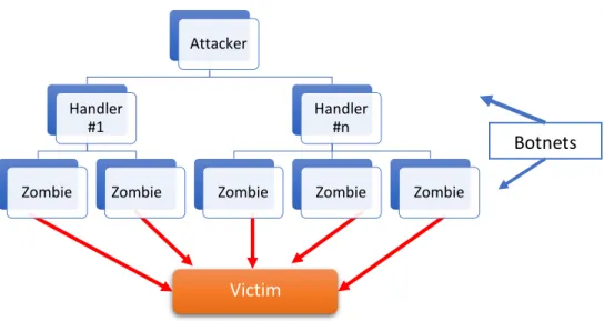
Botnet is the word made from robot and network. Many new bots are working on peer to peer network to communicate in the similar way like client-server but does not requires the centralized server to command [2], [3]. An attacker can choose some of the botnets as ‘handlers’ which can work as command and control functions which in turn provides the instructions to other botnets which will work as zombies and overall form the architecture of the DDoS attack as explained in the figure (see Figure 1). Since zombies, their handlers and other bots are compromised machines in the internet public domain so these machines are under control of attacker which can be used by attacker as and when required. [4][5].

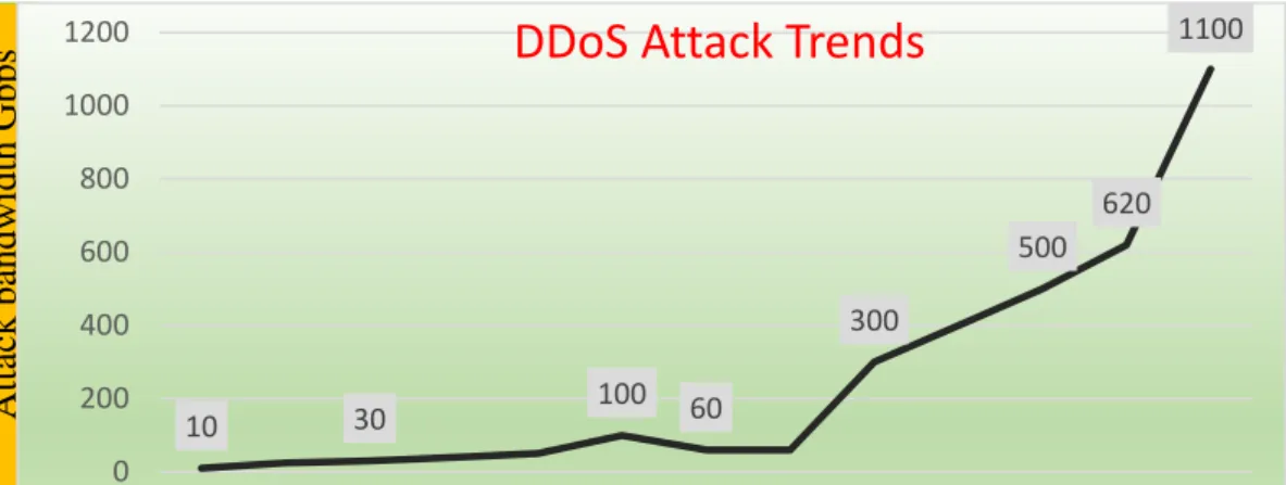
It is evident (see Figure 2) that the Internet botnets development of over the past few years enabled hacker to launch DDoS attacks at a scale higher and higher from the recent one (over terra bytes), which are impossible to stop. Recently in year 2016 Mirai malware has been configured and planned through IoT devices to attack with a disruption potential of 1100 Gbps (1.1 TB) attack on OVH website, which caused many websites like CNN to not function at all. This shows the seriousness of the efforts for research is required to tackle such targeted attacks [3].

Figure 1. Architecture of DDoS attack

Some common types of DoS attacks are given in Table 1

Table 1. DDoS types of attack

S/N Type of DoS attacks Vulnerability exploited / Target 1 Attack on Network

Device

Attacking on hardware and exploiting software bugs in the devices like router etc

2 Attack on Operating System or equivalent levels

Operating System bugs on the level of services and exploiting such services

3 Attack on application or its level

Bugs of software exploited on the application layer 4 Attack through data

flooding

Connection of the servers are limited by the attacking on bandwidth utilization

5 Failure on the Protocol Attacking on the protocol services like spoofing of IP address on the network layer.

Victim Botnets Attacker Handler #1 Zombie Zombie Handler #n

Figure 2. Trends in size of DDoS attacks since 2005 to 2016 in Gbps

2.2. Classification of DDoS

There are many ways in which DDoS classification is done based on criteria like impact size, application layer, attack profile and internet devices communication based on clouds [6], [7], [19]. DDoS attacks can be classified as per the research literature [6] [19]:

2.2.1. Impact Size:

The size of impact on the victim in which it can adversely affect to make it not available to users.

2.2.2. Degrading Network:

It directly affects the services of the victim and make it degraded network and reduce the speed of the network.

2.3. Based on network Vulnerability

DDoS can be classified based on exploiting the network vulnerability [7] or bots available in the network. This can be explained by the attached (see figure 3).

2.3.1. Flood Attack:

In this class of attack network or the machine band width of the victim is brought Year - - - > Attac k ba ndwidth Gbps 10 30 100 60 300 500 620 1100 0 200 400 600 800 1000 1200 2005 2006 2007 2008 2009 2010 2011 2012 2013 2014 2015 09/16 10/16

down to bare minimum or not to be available. Flooding attack can be initiated as direct attack (attack in which Zombies directly affect the victim’s computers) or reflective attack. In this way of attack, reflection is observed in the traffic.

2.3.2. Amplification Attack using DNS:

This is a reflection-based DDoS, in which attacker spoofed up the victim’s IP address to vulnerable DNS server(s) and sends DNS requests using EDNS0 extensions to large DNS messages and cause increased size of requests from 40 bytes to 4000 bytes. This can be further divided in to Smurf and Fragile attack.

2.3.3. Amplification Attack

In such type of DDoS, attacker transmits succession of SYN requests to victim’s machine and consume server’s resources which causing down the system as unresponsive and not responding to the legitimate traffic.

Figure 3. Classification of DDoS by Vulnerability Exploiting [31]

2.3.4. Malformed Server Packet attack

sending modified entries to the IP address of the victim’s machine. This can be further compared in the table 2.

2.4. Countermeasure

There are some countermeasures identified so far now in various researches. Some are proactive and some of them are reactive techniques [2], [8]:

2.4.1. Ingres Filtering:

In this techniques IP addresses are filtered at the router level. Known IP addresses are being blocked before entering the premises of the victim. This can be employed at the ISP and easier to deploy. This has some limitations like 1. IP spoofing,

2. multiple zombies, 3. Its implementation requires additional work at administrator level.

2.4.2. D-Ward

In this technique, firewall is being installed and programmed at the source end networks. Firewall detects such sources originated traffics by collecting information regarding transport and application layers. By analyzing the pre-configured comparison techniques firewall detect and identifies the legitimate and attacker traffic and blocks it at its level. This technique also has some disadvantages like

1. degraded network performance due to computation and filtering algorithms,

2. larger computations tasks to be performed by routers and

3. less efficiency of algorithms performed by the firewalls which may skips new incoming network traffics.

2.4.3. Hop Count Filtering

This technique works on the principle of calculating the time to live (TTL) values which are being inserted by the sender. Difference between the initial TTL value and calculated value at the victim end provides the value of the hop counter. Server at

the victim end measures and calculate the hop counter of various traffics and in this way, it distinguishes the legitimate and the infected traffic. This technique also has some short comings like

1. DHCP pool normally affected by denial of services,

2. techniques does not guarantee the legitimate users which are working being the NAT,

3. sometimes legitimate user’s records (hop counting) are not being maintained

by the server may also face denial of the services.

2.4.4. SYN Cookies:

In this technique server stores the SYN/ACK authentication information instead of storing their Initial sequence numbers. This make this technique as most promising among the other techniques. However, this technique also has some short comings like

1. SYN cookies does not provide robustness, 2. limitation in resending the ACK/SYN packets and 3. excessive utilization of the computing power.

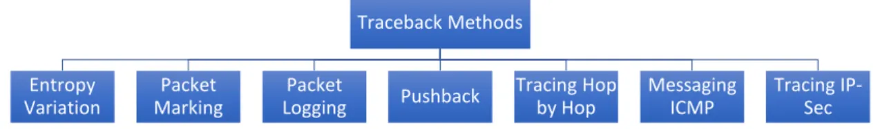
2.5. Trace back technique

Trace back technique DDoS source is being identified though some mechanism and attack vector is isolated before the occurrence of the attack.

Figure 4.Classification of DDoS by Trace Back Technique

2.5.1. Entropy Variation

In this technique difference between the entropies calculated for a normal traffic and under attack traffic.

2.5.2. Packet Marking

In this technique path of the packet is identified from source to destination and marking is done.

2.5.3. Packet Logging

In this technique packet information is stored at each router and being logged. All such routers are teamed together to form a network of sharing this information.

2.5.4. Pushback Mechanism

In this technique, upstream routers are informed about the congestion of the traffic at the downstream routers. This information is being sent to further upstream routers and in case of congestion all upstream routers regulates the traffic to the downstream routers and inhibits the congestion of attack projectile.

2.5.5. ICMP Messaging

In this technique routers are programmed in such a way so that they can to send

Traceback Methods Entropy Variation Packet Marking Packet Logging Pushback Tracing Hop by Hop Messaging ICMP Tracing IP-Sec

the ICMP message with the low utilization of the network traffic.

2.5.6. IP Sec tracing

In this technique authentication of each packet is performed through the shared secret keys. In this way, more secured communication is provided between the terminals.

2.6. Regression Analysis of Network Traffic

Due to severity of the DDoS and its after effects, researchers have analyzed the network traffic statistical analysis for the detection of attack. With the use of regression analysis DDoS attack strength is calculated or estimated with respected to the actual strength. These results are observed as much positive for the routers. There are multiple and polynomial analysis of regression have been used. It has been noticed that combining the various techniques and their effects in suitable circumstances increases the chances of avoiding the DDoS attack [9]. Three different techniques of detection of DDoS identified as:

2.6.1. Profiling of Activity

In this technique header information of the packet is monitored for a proposed network. This helps in calculating the average flow of the packet in the network.

2.6.2. Change Point detection

In this technique network traffic is filtered for fields of IP packets address or protocol and then outcome is stored in the time series, which is a nothing but the outcome of the activity presentation in term of time domain.

2.6.3. Wavelet detection

This is nothing but the monitoring the network performance in the spectral domain of the frequency. During the attack period, some ambiguous signals presence is observed in the spectrum which is equivalent to a signal of noise or the attack.

2.7. Related Work

In study [18] study on botnet performed in IoT devices and networks using deep learning algorithms for detecting the DDoS, LSTM Bayes based methodology has resulted in 98.15% accuracy in the detection of the attack. In LSTM-Bayes algorithm, DDoS attack detected by LSTM technique for higher confidence values and left out low confidence signals are being detected by Bayes method [19]. In some instances where an insider attacker can easily access the system and take controls on the security measure which can lead to the attack proxies. A Moving target mechanism of the protection is proposed to inhibit insiders attacker and load balancing performed on the insider DDoS attack detection which minimizes the proxies involved in.

In software defined network [20] defensive protection framework based on control plane and data plane has been devised. Machine learning techniques used for the detection of the attack in the control plane and at the same time data plan is protected using monitoring algorithm. It has been observed that some of the mechanism of the DDoS detection are working for IPV4 while some of the detection mechanisms are working of IPV6. Researchers [21] proposed protection for IPV6 DDoS attacks, which comprising of mainly ICMP flood attack, can be used. Cloud platforms are vulnerable in current days due to targeted attack of DDoS. Attacker utilizes the vulnerability present in the cloud platforms. Cloud platforms are being detected for DDoS using virtual switch distribution and building monitoring plane shrew attack or flood attack which are comparatively periodic and low in rate normally spectrum template method for the matching and detection is deployed [22]. 3LSTM has resulted 98.42% detection accuracy [13] while LSTM Bayes technique has resulted in 98.12% detection accuracy. Helllinger Distance technique [23] has also been deployed in traffic analysis phase to distinguish between the incoming request and the baseline request for the

network traffic. The threshold of function Hellinger Distance calculation on the incoming packet, it has been detected that the traffic is legitimate or the attack traffic. Attack traffic is dropped and further legitimate traffic packets are being again analyzed based on the on the KDD-99 dataset features extraction. The features are being ranked based on the chi-squared test, information gain and gain ratio calculation. The ranked selected features are outputting a result, which come out as one third of the three filters calculation after the classification performed by J48 classifier. This method has resulted in 99.67% accuracy in detecting the DDoS attack.

Rawashdeh et al.[24] proposed neural network based model using partial swarm optimization (PSO) and enhanced the performance of neural networks. In this methodology the PSO evaluated the optimal weights for each connection which are being used as a feedforward to the neural network. PSO keeps the record of each swarm which would be a probable solution for the entire swarm. For a multimode space swarm particle location is modified based on velocity, gbest (global experience) and pbest (personal experience). While training the neural network error rate is calculated for each particle, which is used to calculate gbest and pbest. The calculation on the particle is performed for the velocity as well as position until the termination criteria is not matched. This methodology proposed a dataset which contains SYN flood, UDP flood and benign packets.

Network security model has been devised [25] for detection of application layer related DDoS attack. A website was created for collecting the dataset records which kept the samples as log of legitimate user and attacking user. Whenever a used access the web, features were recorded in the MySQL database. They derive new features like DT (website’s two successive request time difference from the same source) and BTS (it differential in terms of size in bytes of data for dissimilarity and similarity). Naives

Bayes technique is used for determining the attack or not and resulted in 99% success rate.

CAIDA 2007 dataset has been used by [26] for new algorithm using ensemble methods to select the effective feature from the dataset. In this methodology 7 features are used which are gain ratio, symmetrical uncertainty, chi squared, correlation ranking, information gain and RelieF mainly. Average ranking for each feature and threshold is calculated by the average of all the features ranking. Selection of features is done based on most effective 7 features out of 16 features those crossed threshold value and then applied multiple classifier using weka tool. This method has resulted in 98.3% accuracy.

2.8. DDoS Detection Using Machine Learning 2.8.1. Machine leaning techniques

Modern algorithms of machine learning are used to detect and protect against DDoS especially at the stage of anomaly detection. Currently various used algorithms are Support Vector Machine, Neural Network, K-Nearest Neighbor, Decision Tree, Naive Bayes etc.

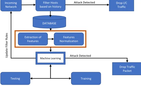
Figure 5 provides an advanced architecture of Machine learning based algorithm utilizing feedback as well as feedforward mechanism to detect the DDoS attack in the network system. In the initial phase traffic of the network is extracted and filtered using defined mathematical criteria or set rules to filter as well as learn as per the stored rules from the defined database. Features are identified and removed from the traffic (for analysis purpose e.g., protocol, byte rate, packet rate in the data stream) in the second step normalization of the extracted features are formed to recondition them for the training process. Training of the neural network will be performed by utilizing the learning algorithms and packet are filtered out from the network traffic as

attacker packet or the legitimate one. Such identified DDoS attacker packets (non- legitimate traffic) are being dropped from the network traffic and algorithm will updates the record for its filtering rules.

Figure 5. DDoS detection Architecture of using machine learning

2.8.2. Deep Learning based of RNN approach

DDoS attacks traffic towards the affected systems get staggered over a period, since it would not look like to be a malicious traffic to the system. Due to this fact the running traffic requires historical information for DDoS detection. We cannot use here detection based on the single packet or its information, moreover it is not enough for the performance evaluation, therefore other historical and stastical patters are to be utilized for detection of the DDoS attack.

Deep Defense approach identifies the DDoS attack identification based on recurrent artificial Neural Network (RNN) e.g. 3LSTM, CNNLSTM, GRU,LSTM etc.

DATABASE Extraction of Features Features Normalization Machine Learning Testing Training Incoming Network Traffic Filter Hosts based on history (Filter) Drop I/C Traffic Attack Detected U p d ate F ilt er Ru le s Drop Traffic Packet Attack Detected

translation, speech recognition, speech synthesis, and other streaming data.

Deep Detection method performs analysis on continuous network packets stream and utilizes learning algorithms to draw a demarcation between the confiscated traffic and legitimate traffic. Information history is used in algorithms of neural network model to separate the legitimate traffic to DDoS attack traffic. Recurrent neural network has advantage of non-dependency on the window size. Window size used to be task-dependent in other algorithms of RNN. This puts limitation on the algorithms to detect the attack. Normally it is has been observed that it is very difficult to train a long-term stream of data to traditional machine learning algorithms. However, this limitation has been overcome by the RNN. RNN has shown given effective results in detecting the attacking packets. Performance increases as the history of the data increases.

Table 2. Comparative of various work done in past to detect the attack

Sr. No Methodology for detection Type of Model used 1 Normal traffic molded in the statistically and

applied to new instances

Statistical modeling 2 Knowing the signatures of the attack based on

various parameters and previous history and their learnings

Knowledge oriented modelling

3 Extraction of features hidden in the flow pattern of network data and building model based on the collected information

Machine learning based on the data mining. 4 Identifying the monitored IDS data for Denial

of Service attack and mis-use detection

DoS type of attack pattern detection.

5 Prediction of the attack based on the data samples of the previous databased derived for the same purpose of DDoS

Centralized anomaly detection

6 Machine learning techniques like K-Naives, CCN, ANN

Machine leaning

techniques and modeling of the attack

7 Advancement to the machine learning and deep learning using stastical parameters along with the attack specific features selection

Deep Learning utilizing Matlab deep learning algorithms

Among all it has been concluded that the optimized machine learning including deep learning method to be utilized for the detection and prediction of the network stream data based on the past data packet learning and applying to filter out the attack packets and passing the benign packets to the premises. This has advantage of lesser CPU time for processing then algorithm, its calculation, lower memory utilization and no extra hardware required for neural network configuration in the communication modules. This will avoid the separate additional hardware requirement for the detection of the attack.

This has multifold advantages over the time to train the network parameters and analyzing the network traffic seamlessly without affecting the resource utilization to great extent. This saves the CPU usage as well as the economically feasible option deployed by all the industries level.

There are various platforms are available for running the deep learning. These are:

Tensorflow: This is developed by google and most popular framework in today’s circumstances. This is being used by Airbnb, Nvidea, Google gmail etc. Python is the mostly used for the programming interface however Java script, C++ and Julia can also be used. This platform requires a lot of coding to achieve the desired learning. In Tensorflow, first graph to be defined first then computation will be performed, that is why it is called static computation graphs also. Tensor flow is good for data integration, graph inputting, images and SQL tables. TF is better choice for cross platform solutions.

PyTorch: This is secondly preferred and in popularity for deep learning, this was developed by Facebook and mostly used by them in own application in addition to Salesforce and Twitter. It contains pre-trained models, supports distributed learning and

data parallelism. PyTorch is better for prototype and small projects. Standard debuggers like PyCharm, pdb can also be used in PyTorch.

Sonnet: This is built on Tensorflow framework, which is designed for neural network and machine learning. Sonnet is used mainly for python objects who are related to neural network. Sonnet produces better results in DeepMind compared to Keras. It’s an abstraction tool which is flexible and competitor to Pytorch and Tensorflow.

Keras: It’s a tool for deep learning if large amount of database available and it

uses minimally Theano or Tensor flow in addition to CNTK. In Keras big models can be configured in few lines of code which makes Keras as less configurable low level framework environment. Prototyping will be less facilitated in the Keras. API of Keras is good in terms of look out, its results are much more readable, although Tensorflow and Keras sits on different platforms, Tensorflow sits at lower lever while Keras at higher level.

MXNet: MXNet is another deep learning scalable platform, which uses a lot of frameworks like Python, JavaScript, Perl, Go, R, Julia etc. This is very much effective platform on multiple GPUs, It has clean and much faster problem solving capability. This make it popular among beginners and experienced programmers.

Swift: This is most popular for app developing in iOS and Mac OS for deep learning swift for TensorFlow is most popular interface. It has very good auto differentiating support which takes derivatives of any function and makes custom structures of data. It has next generation of the API for interfacing, high quality of tooling which is built on LLDB and Jupyter.

Matlab: Matlab has unique tools and they are established. Functionality in deep learning tool box can solve problem easily. This is more suitable for working groups in industry where it is advisable to used commercial licensed products rather than open

source and these open source does not meet the criteria of licensing. Support for Matlab is available from resources while open sources we need to contact community like GitHub. Matlab can import pre-trained models from all other platforms like TensorFlow, ONNX, Keras, Caffe etc. Moreover, Matlab coder can convert standalone C/C++ codes of neural network.

Matlab uses resources more efficiently than listed like python and above, it does not require very high GPU for processing the algorithms. Python like program has many memory errors. We are implementing our model in Matlab because of its better graphical representation of results and better understanding of the iterations and results coming out of it. This will be better understandable for engineers and shop floor operating staffs.

CHAPTER 3: IMPLEMENTATION

Dataset Features extraction and Transformation

It is firstly to separates 20 network traffic features from the dataset of CICDDoS2019 based on the definition and the involvement of the features in detecting the attack which are listed in table 3. These extracted fields are used for training as well as validation purpose. Some of the stastical features used which makes a difference from other machine learning methods where statically data is not used for the analysis purpose. Feature transformation provides a matrix (𝑚𝑥𝑛’), here m is representation of packets quantities and n′ is the representation of new derived features. For learning the patterns for short term and long term, sliding window is used to distinguish continuous packet and reassemble them in a window size of T. Label of every window denotes the last packet. Feature Extraction and Transformation shapes stream into a three-dimensional matrix with size (𝑚 − 𝑇)𝑥𝑇𝑥𝑛’. This way, the features are converted to window instead of a packet, this help in learning the network patterns from the previous packet sequence.

Figure 6. Single directional RNN [46]

Bidirectional RNN consists of two RNNs sequence to sequence. RNN layer provides the trace of the history from the previous packets. LSTM and GRU both techniques are used for the purpose of eliminating the history. Thus, observed new LSTM contains three gates for every cell which are forget, input and output. Mathematically it can be expressed in following equations:

𝑖𝑡 = 𝜎(𝑊𝑖 ⋅ [ ℎ𝑡 − 1 , 𝑥𝑡] + 𝑏𝑖) 𝐶˜𝑡 = 𝑡𝑎𝑛ℎ(𝑊𝐶 ⋅ [ ℎ𝑡 − 1 , 𝑥𝑡] + 𝑏𝐶) 𝑓𝑡 = 𝜎(𝑊𝑓 ⋅ [ ℎ𝑡 − 1 , 𝑥𝑡] + 𝑏𝑓 ) 𝐶𝑡 = 𝑓𝑡 ⋅ 𝐶𝑡 − 1 + 𝑖𝑡 ⋅ 𝐶˜𝑡 𝑜𝑡 = 𝜎( 𝑊𝑜 ⋅ [ ℎ𝑡 − 1 , 𝑥𝑡] + 𝑏𝑜) ℎ𝑡 = 𝑜𝑡 ⋅ 𝑡𝑎𝑛ℎ( 𝐶𝑡)

Where 𝑥𝑡 is the input at time 𝑡 , 𝑊𝑖, 𝑊𝐶, 𝑊𝑓, 𝑊𝑏 are weight matrices, 𝑏𝑖, 𝑏𝐶, 𝑏𝑓 , 𝑏𝑜 are biases, 𝐶𝑡, 𝐶˜𝑡 are the new state in the memory cell, while 𝑜𝑡 and 𝑓𝑡, are output gate and forget gate. There were 64 Neurons were used in the sequence, whose output is described as a function

𝑓( 𝑥) = 𝑡𝑎𝑛ℎ( 𝑥) While output of the sigmoid function is 𝑓( 𝑥) = 1

1+𝑒𝑥

CHAPTER 4: DATA COLLECTION

4.1 Results of collection of Data

Five steps are taken to achieve the desired results as listed in the motivation part. This has been illustrated below in details. Fine tuning of the data set has been done at various level from selection of the data to features and processing of the features to accommodate in the Matlab platform. Many features are included which are naïve of the communication setup for a TCP/UDP while some of the features are stastical in nature and included to support the calculation of the desired accuracy.

4.1.1 Collection Phase of Data

In this phase datasets are collected from various sources which are suitable for proofing the postulate of detection of the DDoS. Evaluation of new DDoS techniques and algorithms heavily depends on the dataset quality to suit the application and computational techniques used in generating the dataset features.

(a) Dataset requirement: New DDoS attacks are employing newer techniques and amount of attack load on the victim is mainly happening in the range of terra bytes/sec. Dataset selection also depends on the different types of DDoS attacks and their impact on the victim, approach used in the network flow for data and protocols used for the attack.

Reflection DDoS are causing the multifold impact which became impossible for a victim computer to handle. So, all these characteristics have been not possible in one type of data sets, therefore strategy adopted to use datasets which have most of the DDoS families components and all previous shortcoming of various researches are eliminated in those one.

(b) Dataset Availability: Following are the referenced dataset used for the detection of the DDoS which are generated by University of Brunswick Canada CIC

recently in year 2015, then refined in 2017, 2018 and in year 2019 published CICDDoS2019. We used combination of all the datasets in evaluating the model proposed considering different DDoS pattern generated in each refinement of publication.

Firstly, experiment done on individual and later optimized dataset prepared which utilizes the all classified DDoS family members.

(c) Dataset Source: The link https://iscxdownloads.cs.unb.ca/iscxdownloads stores the latest and previous datasets generated by UNB and Canadian Institute for Cybersecurity (CIC). These are free to download and made available for the research in the same field. It has been observed that datasets are refined every year for new type of threats developed are being addressed in the latest dataset published in year 2019. We utilized them for training of our model and further details follows in the coming section.

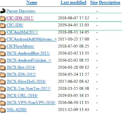
The link also contains data sets for experiments performed in year 2017, 2018 and 2019.

4.1.2 ISCX NSL-KDD

Above mentioned dataset includes enough data records for training and testing. Although data records are in abundance and do not have redundant records so false detection of the attack can be avoided and prevent model to learn them and hence higher accuracy of the learning results. Above listed are the data which included in the zip folder for NSL-KDD dataset [9]. Other datasets are built in year 2015 -2016 and after that the intensity of the attack has been increased in multifold so of less use but indicative of representation for DoS. Therefore, these are being used for reference and initial verification of the other results to achieve accuracy.

4.1.3 Datasets for year 2017

Figure 9. ISCX link content for CIC2017.

This is the folder from where the dataset CIC-IDS-2018 is downloaded for testing and training of the proposed model. List of files containing in this folder are listed as below:

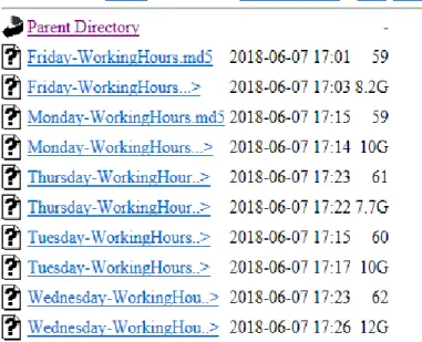
Figure 10. ISCX 2017 dataset

Dataset ISCX 2017 contents and relevant files are available at link https://iscxdownloads.cs.unb.ca/iscxdownloads/CIC-IDS-2017/PCAPs/.

In this folder file “Friday-Working hours-Afternoon.pcap” contains the data for the DDoS attack. Total 8.2 GB of data is there out of which extracted file through Wireshark is containing the 85 columns and selective 225746 rows of data that has been converted to .csv format for easier upload in the offline training module of the Matlab.

Table 3. Features selected from dataset.

S/N Features Attack Profile

1 Source IP DDoS

2 Source Port DDoS

3 Destination IP DDoS

4 Destination Port DDoS

5 Protocol DDoS

6 Timestamp DDoS

7 Flow Duration DDoS

8 Total Fwd Packets DDoS

9 Total Backward Packets DDoS 10 Total Length of Fwd Packet DDoS 11 Total Length of Bwd Packets DDoS 12 Fwd Packet Length Std DDoS

13 SYN Flag Count DDoS

14 RST Flag Count DDoS

15 PSH Flag Count DDoS

16 ACK Flag Count DDoS

17 Fwd Header Length DDoS

18 act_data_pkt_fwd DDoS

19 Bwd Packets DDoS

Table 4. Features Description in details [5], [7] on datasets

S/N Feature Feature Description

1 Source IP IP address of Source

2 Destination IP IP address of Destination or victim 3 Source Port Port number at Source end

4 Destination Port Destination port number

5 Flow Duration Flow of packets (number/seconds) 6 Protocol Protocol used for the communication

7 Time Stamp Time of communication

8 Total Fwd Packets Total number of forward direction packets sent 9 Total Backward Pkt Total number of backward direction packets sent 10 Fw Pkt L Max Maximum length of forward packet

11 Bkw Pkt L Max Maximum length of Backward packet 12 Fw Pkt L Min Minimum length of forward packet 13 Bkw Pkt L Min Minimum length of Backward packet 14 Fw Pkt L Average Average length of forward packet 15 Bkw Pkt L Average Average length of Backward packet 16 Fw Pkt L Std Std Dev Size of forward packet 17 Bkw Pkt L Std Std Dev Size of Backward packet 18 Flow Byte/Sec Flow in terms of Bytes/secs 19 Flow Packets/Sec Flow in terms of packets/sec

20 Flow iat avg Average time between the two packets 21 Flow iat std Std Dev time between the two packets 22 Flow iat max Max time between the two packets 23 Flow iat min Min time between the two packets

24 Fwd iat avg Average time between the two forward packets 25 Fwd iat std Std Dev time between the two forward packets 26 Fwd iat max Max time between the two forward packets 27 Fwd iat min Min time between the two forward packets 28 Bkw iat avg Average time between the two Backward packets 29 Bkw iat std Std Dev time between the two Backward packets 30 Bkw iat max Max time between the two Backward packets 31 Bkw iat min Min time between the two Backward packets 32 Fwd Push Flag No of Push Flag when pkt sent in f/w direction 33 Bkw Push Flag No. of Push Flag when pkt sent in b/w direction 34 Fwd URG Flag No. of URG Flag when pkt travel u/p direction 35 Bkw URG Flag No. of URG Flag when pkt travel in b/w direction 36 Fwd Header Length Forward Header Length

37 Bkw Header Length Backward Header Length 38 Pkt Length Max Maximum Length of Flow 39 Pkt Length Min Minimum Length of Flow 40 Pkt Length Avg Average Length of Flow 41 Pkt Length Std Std Dev Length of Flow 42 Pkt Length VA Inter-arrival of packet flow 43 FIN Count FIN Counts of Packets

Table 4. continued...

S/N Feature Feature Description

45 RST Count RST Counts of Packets

46 PST Count PST Counts of Packets

47 CWE Count CWE Counts of Packets

48 ECE Count ECE Counts of Packets

49 Up and Down Ratio Upload and Download ratio 50 PKT Size Avg Average size of Packet

51 Fwd Segment Avg Forward Segment average size 52 Bkw Segment Avg Backward Segment average size 53 Fwd Byte Blk Avg Forward Byte rate average 54 Fwd Pkt Blk Avg Forward Packet rate average 55 Fwd Blk Rate Avg Forward Bulk rate average 56 Bkw Byt Blk Avg Forward Byte rate average 57 Bkw Pkt Blk Avg Forward Packet rate average 58 Bkw Pkt Rate Avg Forward Bulk rate average

59 SUB Flow Fwd Pkt Forward Average number of Subflow of packet 60 SUB Flow Fwd Byte Forward Average number of Subflow of Bytes 61 SUB Flow Bkw Pkt Backward Average number of Subflow of packet 62 SUB Flow Bkw Byte Backward Average number of Subflow of Bytes 63 Fwd WIN Byte No of bytes sent in Forward direction to initialize 64 Bkw WIN Byte No of bytes sent in backward direction to initialize 65 Fwd Actual packet Forward direction >1 byte data payload

66 FWD SEG Min Forward direction Minimum segment observed 67 ATV average Average time to become active flow to idle 68 ATV Std Dev Std Dev time to become active flow to idle 69 ATV Max Max time to become active flow to idle 70 ATV Min Min time to become active flow to idle

71 IDLE average Average time to become active flow before idle 72 IDLE St Dev Std Dev time to become active flow before idle 73 IDLE Max Max time to become active flow before idle 74 IDLE Min Min time to become active flow before idle

4.1.4 CIC-IDS 2018

Second data set collected from UNB Canada which was generated in year 2018 considering the limitations of the available previous dataset to map the DDoS attacks. These are listed as CIC IDS 2018. This dataset consists of modern DDoS attack scenarios which includes Web attacks, Heartbleed, DoS, Web attacks, Brute force,

botnet and various infiltration activities inside the network performed by out of the network attacker. To generate this dataset, infrastructure of about 50 machines were used to attack the victim who has an organization of 420 machines, 30 servers and consisting of 5 different departments. Team captured network traffic and logs of each computer. They derived 80 features from the logs generated and published in the form of .pcap files as well as .xml files for the use. These are downloaded from the address https://iscxdownloads.cs.unb.ca/iscxdownloads/CIC-IDS-2017/. Content of the location are mentioned in figure 11.

Figure 11. CIC Dataset 2018 location contents

These datasets are also being utilized in detection of the attack using the model derived in the Matlab platform. Results are discussed in the discussion section.

4.1.5 CICDDoS2019 dataset from UNB

CICDDoS2019 dataset developed by Iman [5] at university of Brunswick Canada, which is comprehensive and including proposed new taxonomy for the detection of the DDoS attack. This dataset addressed the shortcomings of the previous other published

sums to all 13 types of the attack patterns included in the data set with benign samples. Attack included are Reflection Based attack data (MSSQL, SSDP, DNS, LLDAP, NETBIOS, SNMP, PORTMAP) and exploit based data (SYN Flood, UDP Flood, UDP Lag). Data samples were collected from the firewall which is called as CICflometer-V3 in the form of PCAP files and for the analysis purpose .csv files also made available. These data are arranged day-wise experiment done by the team on two days (day1 and day2) with 80 features.

We utilized this dataset for the comparing the previous published dataset. Our model was run on these datasets with 20 features extracted out as mentioned in the table 3.

4.2 Segmentation of Data and cleansing

Data segmentation is a task in which datasets data are divided into the groups of similar data for example same type of attack like Heart Bleeding, Fire Eye, NetBIOS, UDP, MSSQL, DNS, LDAP etc. and clubbing effective proper samples of each type of attack. All data records which are not replicative and not effective are being discarded, since the selected datasets are having more than 1 million of the data records hence it is very essential to choose the records which happened in a small amount of time and effective results of the DDoS attacks are being resembled after scrutinizing them. As we observed that DDoS based in literature review has mainly two types of attacks reflection type and exploiting the resource type, counts to 13 types are included in this dataset.

All different type of attacks has unique meta signature in terms of the feature parameters. After analyzing the attack patters of most of the DDoS attacks out of 85 features only 20 features are selected which can form the signature of the attack in the dataset record. Such all resembling records are categorized for each 13 types of the attacks and combined to form a single dataset for the training and validation as well as

for the measurement.

These collected datasets which are grouped in a single test dataset are being divided into sub datasets of different sizes of 2500, 7500, 15000 up to 200,000. More than 133723 records being utilized to train different training models. Each dataset size has the similar data for labels. Only 20 features were extracted out of all the listed 85 dataset features. Model run on all the record set to check and get the optimized desired result. It has been observed that as the number of records of the dataset increases number of epochs are increasing and the gradient of the results is increasing.

4.3 Pre-Processing of Data

In this phase, 2-D vector training and testing were changed to the vector format so that it can be acceptable to the neural network algorithms. Those records which has number in it and zeros are being converted to floating point numbers. All the IP addresses were converted into the numbers using binary to numerical value. For example, 192.168.100.10 is converted to 192x2563 _+168x2562 _{+ 100x256 + 10 =}

3232261130, while at the same time and date & time stamps are also being converted to a numeral of decimal point. This step is required for quantifying the intensity of the attack in terms of data flow and its weighted network resource utilization to make it fail for the other customers and flooded and make it victimized. Same way destination IP address has also been converted to numerical value. This way IP addresses were normalized in the table and contained in the CSV format.

4.4 Neural network Training and Testing Phase

The vectorized dataset derived from the above step (segmentation, cleaning) has been used for the training and testing purpose in the Matlab based Neural Network algorithm. In this phase of training, various parameters such as dataset size, weights, epoch, biases, nodes, and learning rate are configured,

while in the validation phase mean square error, accuracy and cost are being monitored for the optimized detection accuracy.

4.5 DDoS attacks Classification

Hot encoded process is being utilized for all detected DDoS flooding attacks by Matlab artificial neural network Algorithm in which number 1 represented as attack, and non-DOS data records are being expressed as 0 in all normal packets. This methodology has been adopted for easier interpretation of data when the model simulation runs successfully in Matlab. The embedded graphical visual aspect of Matlab used for the easy interpretation of the results. This is used to determine the DDoS attacks detection and various other similar DDoS types characteristics.

CHAPTER 5: DISCUSSION

Results of neural network fitting has been displayed in the picture form in the below section. Experiment performed with various lengths of the dataset record lengths and number of the features. Main purpose of the selection of the features is to optimize the metadata for detection of the attack based on the network traffic. In the first set of models run, total 191033 samples were inserted out of which 15% each were used for the purpose of the training and 15% records for validation by the model.

It has been resulted from the models test run that the accuracy of 100% detection has been achieved with limited number of 20 features (optimized from 85) with normalization. There is no need of 85 features to detect the attack. All the selected features were based on the theory of the modern attack pattern, in which the attack traffic will be looks like the legitimate traffic. Lesser the features faster the detection and earlier the action to reject the incoming heavy traffic. This enables the quick remedial of the attack upfront with the help of feedforward and feedback-based system responses. Feedback will be received from the learned data after passing through the model while feedforward action will be taken immediately based on the past learned data (history). Hence the attack effect will be null at the victim computer system or the network. This is explained with the help of the data model training and validation results in the below paragraphs.

It has been also observed that the higher the value of the records in the dataset for the training and validation of the results, function fits for the outputs and all three graphs (training, testing and validation) follow each other exactly in the same manner. Also, it has been noticed that up to 20,000 data records in the dataset give the max results with the 100% accuracy with the 20 numbers of the optimized selected features. Experiment also performed on the 45 number of the features out of 85, but

results remains the same except the greater number of iteration and epochs utilized by the model, this shows that the higher the number of the features, accuracy remains the same but more CPU resources and time required to train the model. Hence it is of no use to use higher number of the features and experiment limit to the table 3 listed features only. Results are same, lower CPU usage and faster results while the accuracy comes the same from the same classifier of training records (if selected higher features).

Table 5. Model Configuration

Parameter Specs 01A Specs 01B

Dataset base ISCX2017 CICDDoS2019

No of Samples 191033 222257 Training Sample (70%) 133723 (60%) 133355 Validation Samples (15%) 28655 (20%) 44451 Testing Samples (15%) 28655 (20%) 44451 No of Neurons 10/20/40/80 10/22/44/88 No of Features selected 20 22 Hidden Layer 2 2 Output Layer 1 1 Algorithm LM SCG

Performance mean sq. error cross-entropy

Type of attack DDoS DDoS

DDoS Variants 7 13

One more observation noticed, that if the all dataset features (85) are used as it then there is no result plotted by the model (means fails). So, optimization in selection of data records of the dataset as well as the features as well as normalization is necessary or important parameters for the efficiency to achieve. Based on the above two datasets ISCX2017 and CICDDoS 2019 model designed in algorithm is detailed in table 5.

The word DeepDefence means a deeper analysis of the data utilizing all the possibilities and techniques of the Machine Learning to detect the attack with higher success rate and faster (in short time) to take proactive mitigating steps by the model

itself before the user get victimized. This process will be transparent to the end user and he will be not get affected while the model will reject all the malicious source IPs addresses at the gate of the network. The objective of the work is to optimize the CPU utilization during the learning process and at the same time efficiency on detection to be achieved, we would start implementing using neural network and going on checking the other machine learning and deep learning techniques till the desired efficiency achieved then work further experiment will not be performed. Another object is to utilize the small memory utilization to optimize the work on a small GPU based circuit board or in the communication module of the industrial control systems.

Model test with CIC2017 dataset samples (dataset 01A)

Model run with 15% of validation and 15% for training.

Figure 12. Model Configuration

analysis. Out of which 15% samples which counts to 28655 were used for the purpose of validation and 15% samples used for the purpose of testing, while remaining 70% samples which counts to 133723 were used for the purpose of the training the model.

Architecture of the neural network

Architecture of ANN is with 10 hidden layers and one output layer. This has run in 2 stages. We have performed the testing with number of hidden layers variation from 20 to 120 in multiples of the features, but the end result remains same so considering the optimized value of 10 as hidden layers for effective utilization of the computing. Output was configured as single either DDoS affected sample or benign sample, or in other words result was selected as binary in terms of 1 as attack while 0 as benign.

Training of the network performed through Levenberg-Marquardt training algorithm

For the purpose of the training the network various options of selection of the training models are available in the Matlab code. Levenberg-Marquardt back propagation model is used for the coding purpose in our experiment setup. In back propagation model Jacobian performance is calculated with the values of the bias and its weights. The advantage of selecting this model is that it stops automatically if of the following condition is being satisfied:

(a) If the gradient of the performance is falling below the set value min_grad in code (b) Epochs or repetitions are reached to the maximum value

(c) Time to train the model exceeds the maximum time allotted

(d) Performance of the model is getting reduce below the minimized goal

Result 1

Figure 15. Result from model configured (see section 5.1.1)

Results obtained shows the gradient as 1.42 and only 3 numbers of iterations have derived the desired results with the accuracy of almost near to 1.0

Plot of the samples

On plotting the testing data, validation data and output data on the plot it has been observed that it exactly fits one on to another. Which is the symbol of no error.

Figure 16. Function Plot for Output element

This plot (figure 16) is showing the testing, training and validation results obtained on the target values, which fits perfectly each other on the desired results. It shows that model depicts that the graph is nonlinear in nature and training targets, validation target and test targets are being overfitted.

Regression Plot Setup -1

Regression graph is appearing with grading at almost equivalent to R=1.0, in all the training, validation and Sample data as well as output data.

Figure 17. Regression Plot

Regression plot (figure 17) shows that the data samples filtered out and mathematically adjusted offline are contributing factors to the achievement of the desired accuracy.

Performance of the network

Accuracy has been observed from decimal of 1% to accurately detecting the attack.

Figure 18. Validation Performance Curve

Validation performance is plotted against the number of the iterations. It has been observed in the result that the maximum performance is achieved with the 3 numbers of the epochs. The further calculation of the training the model stops as the desired results has been obtained as the Levenberg-Marquardt model coded.

Network training & validation gradient

Various parameters of the Levenberg-Marquardt algorithms were displayed in the graphs (figure 19) which are gradient, mu and fall in the value as the number of the epochs increases.

Figure 19. Network training gradient and Validation checks

Set-up 2 CIC dataset samples with higher % of training and validation

Testing and validation performed with max 35% of the dataset samples, in which only 30% of data samples are used for the training purpose. In this setup training and validation samples were increased from 15% to 35% to achieve better validation and training and observe the model training with 30% of the samples. This is just to notice the effect on the achieved accuracy if the training samples were decreased from

133723 to 57309 samples for training purpose while the validation and testing samples were increased up to 66862 samples each.

Figure 20. Experiment setup 2 Modelling

Results of setup 2:

For the calculation purpose and comparison, the number of the hidden layers were again restricted to 10 only as it was not making any impact on the performance as well as accuracy of the model. In this test we achieved gradient of 1.66 and epochs remains 3 for the desired accuracy achievement.

Figure 21. Result of setup 2

It has been observed that (figure 21) the accuracy with lower number of samples has also been achieved with the desired results. The advantage of using Levenberg-Marquardt algorithm has been displayed here because this algorithm uses both methods of estimation which are Gaussian-Newton method as well as the gradient descent rule. Levenberg-Marquardt utilizes the principle of using large number of samples in the first iteration to decide the step size and then later uses lesser number of the samples in later stages of the iterations. Thus, result will start converging from the first result to the later results with better accuracy or minimum error (gradient descent) and at the same time avoids the errors in the Gaussian-Newton method.

Plot fitting is observed as perfect matching

In experimental setup 2, the graph (figure 22) is overfitting fitting and covering the training targets over the sample targets at the same time validation and test targets are being covered by validation and test targets respectively. Error has been displayed near to the zero and a straight mark is appearing which shows the accuracy achieved by the training the model.

Figure 22. Function fit for output element.

ROC and Confusion matrix

ROC (Receiver Operating Characteristic of Curve) is the indication of the positive rate over false rate for each sample set of training, testing and validation sample in the dataset. ROC provides the sample set to be considered for selection of the optimal

sets over the suboptimal sets, which needs to be discarded. The positive rate is the indication of the sensitivity of the dataset representation towards accurate detection which is also known as the probability of the detection of the attack.

Figure 23. RoC for Setup 2

Training, validation test and all ROC are moving through the true positive rates and they are not being deflected towards the false positive rates, which is the indication of the lesser errors in the detection of the attack by the model proposed based on the set of the samples provided for training the model.

Confusion Matrix:

Confusion matrix portrays the performance of a classifier ( Classification model) over the proposed dataset samples with known results. Our matlab code plots confusion matrix of 3x3 size for each of the class model viz. training, validation and test. An overall confusion matrix also plotted for over all results of the feeded classifier. Since our output class has been defined with binary result either 0 or 1 so results were plotted in the confusion matrix with both results detection with their accuracy. This is repeated with all three classes of training, validation and test. First row represents the detection of result 0, while second row represents result of 1 detection and third row indicates the % of detection with accuracy and false positive cases accuracy.

Validation Performance

Validation performance curve is the representation of the type of configuration change in the model requires to predict the accuracy of the model. These curves may be under fitting, over fitting or good fitting curve. In our case the model is representing an over fitting characteristing means it is able to understand the losses, noise and complexity of the dataset employed. If distance between the curves of training and validation increases then it is indication of more losses and greater noise present in the sample medium. If distance is lesser and goes up and down then it is the representation of the good fitting and if one curve overlays over the another then it is example of overfitting in which the noise, errors in dataset and accuracy of features presented has been well learned by the model.

Model with samples from dataset 01B, CIC2017-2019

To overcome the suspicion and to get the results with lower number of samples to understand the prediction of the attack by the proposed model, another experiment has been performed with the combined data samples from all datasets (2017 to 2019), to meet the requirement of detection of attack without compromising the accuracy in the detection. This has been the worst-case scenario to check the performance of the model proposed in detecting the attack. Although there are variations in the dataset on their features so exercised made to get the same features used for previous experiment (representing all the attack types inclusion and selection of 20 most representative features as per table 3 among 80 features listed in table 4 in the dataset)

Test Samples and distribution among Training and Validation

Total 222,257 samples were selected which comparises of all the types of attacks on which the data set were prepared (figure 26).

20% samples were selected for testing and 20% samples were used for the validation of the results, remaining 60% samples were used for the training the model.

Modelling and network architecture

Same 20 features as described in table 3 were being used for the selection among 80 total features provided by the dataset. Hidden layers kept same as 10, due to the fact that this has not impacted on the results as noticed in previous experiment.

Output layer also defined to 1 to get the result in binary whether incoming packets are belongs to an attack traffic or a benign traffic. Output 1 represents an attack while output 0 represents a benign.