Cross-dynamics of volatility term structures implied by foreign exchange options

WO R K I N G PA P E R S E R I E S

N O. 5 3 0 / S E P T E M B E R 2 0 0 5

CROSS-DYNAMICS OF

VOLATILITY TERM

STRUCTURES IMPLIED

BY FOREIGN EXCHANGE

OPTIONS

In 2005 all ECB publications will feature a motif taken from the €50 banknote.

W O R K I N G PA P E R S E R I E S

N O. 5 3 0 / S E P T E M B E R 2 0 0 5

This paper can be downloaded without charge from http://www.ecb.int or from the Social Science Research Network electronic library at http://ssrn.com/abstract_id=804944.

CROSS-DYNAMICS OF

VOLATILITY TERM

STRUCTURES IMPLIED

BY FOREIGN EXCHANGE

OPTIONS

by Elizaveta Krylova

_{, Jussi Nikkinen}

and Sami Vähämaa

1 We wish to thank Vincent Brousseau, Jenni Ipatti, Benjamin Sahel, Alain Vandepeute, an anonymous referee, and the Editorial Board of the ECB Working Paper Series for valuable comments and suggestions. Nikkinen and Vähämaa gratefully acknowledge the support of the Emil Aaltonen Foundation and the Evald and Hilda Nissi Foundation.The views expressed in this paper are those of the authors and do not necessarily reflect the views of the European Central Bank.

© European Central Bank, 2005 Address

Kaiserstrasse 29

60311 Frankfurt am Main, Germany Postal address

Postfach 16 03 19

60066 Frankfurt am Main, Germany Telephone +49 69 1344 0 Internet http://www.ecb.int Fax +49 69 1344 6000 Telex 411 144 ecb d

All rights reserved.

Any reproduction, publication and reprint in the form of a different publication, whether printed or produced electronically, in whole or in part, is permitted only with the explicit written authorisation of the ECB or the author(s).

The views expressed in this paper do not necessarily reflect those of the European Central Bank.

The statement of purpose for the ECB Working Paper Series is available from the ECB website, http://www.ecb.int.

C O N T E N T S

Abstract 4

Non-technical summary 5

1 Introduction 7

2 OTC currency option data 11

3 Descriptive statistics and preliminary analysis 13

4 Empirical findings 19

4.1 Common factors of implied volatility

term structures 19

4.2 Innovation accounting and variance

decompositions within a VAR framework 24

4.3 Linear and nonlinear causality 30

5 Conclusions 37

Appendix 39

References 41

Abstract

This paper examines the cross-dynamics of volatility term structures implied by foreign exchange options. The data used in the empirical analysis consist of daily observations of implied volatilities for OTC options on the euro, Japanese yen, British pound, Swiss franc, and Canadian dollar, quoted against the U.S. dollar. The empirical findings demonstrate that two common factors can explain a vast proportion of the variation in volatility term structures across currencies. Furthermore, the results indicate that the euro is the dominant currency, as the implied volatility term structure of the euro is found to affect all the other volatility term structures, while the term structure of the euro appears to be virtually unaffected by the other currencies. Finally, our results reveal a rather deviant relation between the volatility term structures of the euro and Swiss franc by providing evidence of significant nonlinearities in the relationship between these two currencies.

JEL classification: F31; G13; G15

Non-technical summary

Option prices implicitly contain information about market participants’ volatility expectations. These volatility expectations implied by option prices typically differ across times to maturity of option contracts, and thereby form a term structure of volatilities. The purpose of this study is to examine the cross-dynamics of volatility term structures implied by foreign exchange options. This analysis is motivated by the existing literature, which demonstrates that volatilities are closely linked across currencies. Furthermore, previous studies have also noted that volatility term structures implied by foreign exchange options tend to be rather similar across currencies. Using a comprehensive data set of over-the-counter options on the euro, Japanese yen, British pound, Swiss franc and Canadian dollar vis-à-vis the U.S. dollar, this paper examines whether implied volatility term structures are affected by common uncertainty factors, and moreover, whether any causal dynamics are present among the term structure time-series.

The results of this analysis demonstrate that the implied volatilities of major currencies exhibit considerable term structure behavior. For the euro, British pound and Swiss franc, the implied volatilities of longer maturity options exceed, on average, the volatilities of shorter maturity options, while the implied volatilities of the Japanese yen and Canadian dollar appear to decrease with time to maturity. However, it is also found that implied volatility term structures vary heavily over time. Although the volatility term structures of the European currencies tend to be upward sloping, sustained periods of downward sloping term structures can also be observed.

Furthermore, the empirical findings of this paper indicate that implied volatility term structures exhibit somewhat similar patterns over time. The term structures of the European currencies, in particular, are found to be closely linked with each other. Our findings also suggest that a vast proportion of the variation in volatility term structures across currencies can be explained by two common factors. These two factors, however, describe the dynamics of the European volatility term structures more adequately than the dynamics of the Japanese yen and Canadian dollar implied volatilities.

The results of this paper also show that the volatility term structure of the euro has a leading role in the system of term structures. It is found that the implied volatility term structure of the euro considerably affects all the other volatility term structures,

while the term structure of the euro appears to be virtually unaffected by the other currencies. Finally, the empirical analysis presented in this paper reveals a rather deviant relationship between the volatility term structures of the euro and Swiss franc. Besides demonstrating a very tight linkage between the volatility term structures of the euro and the Swiss franc, our results also provide evidence of significant nonlinearities in the dynamic relationship between these two currencies. This relation may, for instance, partially reflect the leading role of the euro and the “safe haven” property of the Swiss franc.

The empirical findings reported in this paper have important practical implications for financial market practitioners, such as option traders and risk managers, and also for monetary policy and bank supervision authorities. Knowledge of the common factors and causal dynamics of implied volatility term structures may be useful for formulation and implementation of investment and risk management strategies. The leading role of the euro, for instance, may be utilized for improving volatility forecasts that are needed in various financial applications. The results of this paper may also be of interest to central banks, as the documented linkages in volatility term structures indicate that exchange rate volatility expectations are strongly affected by global uncertainty factors which are beyond the control of local monetary policy.

1. Introduction

Since the price of an option is decisively determined by the market’s assessment of the volatility of the underlying asset over the remaining life of the option, market prices of options implicitly contain information about market participants’ volatility expectations. Consequently, given an option pricing model, these volatility expectations implied by option prices can be extracted.1 Most conventionally, the Black-Scholes (1973) / Merton (1973) option pricing framework is applied to extract volatilities, and hence implied volatility is typically defined as the value of standard deviation of the underlying asset price process that produces the observed market price of an option when substituted into the Scholes option pricing formula. Although the Black-Scholes model assumes constant volatility, this assumption is obviously not made by the market.2 It is now well known that implied volatilities differ across times to maturity of option contracts, and thereby form a term structure of volatilities (see e.g., Heynen et al., 1994; Xu and Taylor, 1994; Campa and Chang, 1995).3 Given that implied volatility may be regarded as the market expectation of future volatility, differences in implied volatilities across times to maturity should reflect differences in market participants’ perceptions of uncertainty over given future horizons.

Despite the vast empirical work on implied volatility, surprisingly little attention has so far been devoted to the term structure of implied volatilities. The basic time-series properties of implied volatility term structures have been examined e.g. in Stein (1989), Diz and Finucane (1993), Haynen et al. (1994), and Xu and Taylor (1994). Stein (1989) reports evidence of consistent over-reactive behavior in the volatility term structures implied by S&P 100 index options. Diz and Finucane (1993), Haynen et al. (1994), and Xu and Taylor (1994), however, document contradictory findings and

1 _{Provided that market participants are rational, implied volatility should incorporate all the available} information that is relevant for forming expectations about the future volatility. Therefore, implied volatility is widely considered to be the best available estimate of market uncertainty.

2 _{However, the Black-Scholes model is valid even if volatility is allowed to be a deterministic function of}

time (see e.g. Merton, 1973). In this case, the constant variance parameter used in the Black-Scholes formula is replaced by the expected average variance over the remaining life of the option.

3 _{It is also well known that the Black-Scholes implied volatilities differ across strike prices (see e.g.,} Rubinstein, 1994; Mayhew, 1995). This variation of volatilities across strike prices is commonly referred to as the volatility smile or volatility smirk.

conclude that volatility expectations behave rationally. Das and Sundaram (1999) compare the implied volatility term structures produced by two competing classes of stochastic processes. They find that jump-diffusion models produce implied volatility term structures that are always upward sloping, while stochastic volatility models, in turn, can produce a wider variety of patterns of term structures.

Since volatility term structure is, in principle, analogous to the term structure of interest rates, previous studies have noted that it may provide information about expected future short-term volatilities. This expectations hypothesis is explicitly tested in Campa and Chang (1995). Using volatilities implied by foreign exchange options, Campa and Chang (1995) are unable to reject the expectations hypothesis, thereby demonstrating that the volatility term structure is useful for predicting future short-term volatilities. Consistently, Xu and Taylor (1994) also show that volatility term structures are useful for volatility forecasting purposes. The dynamics of implied volatility term structures have recently been examined in Mixon (2002). Using data on S&P 500 index options, Mixon (2002) demonstrates that variation in volatility term structure over time can be explained at least to some extent by common factors, such as observable economic fundamentals.

The purpose of this study is to examine the cross-dynamics of volatility term structures implied by foreign exchange options. This analysis is motivated by the existing literature, which demonstrates that volatilities are closely linked across currencies (see e.g., Najand et al., 1992; Fung and Patterson, 1999; Kearney and Patton, 2000; Speight and McMillan, 2001). Furthermore, Xu and Taylor (1994) have previously noted that volatility term structures implied by foreign exchange options tend to be rather similar across currencies. Using a comprehensive data set of over-the-counter options on the euro, Japanese yen, British pound, Swiss franc and Canadian dollar vis-à-vis the U.S. dollar, this paper examines whether implied volatility term structures are affected by common uncertainty factors, and moreover, whether any causal dynamics are present among the term structure time-series.

This paper contributes to the literature in several respects. Most importantly, to our knowledge, this paper is the first attempt to address the cross-dynamics of implied volatility term structures. This analysis is considered to provide new insights into the behavior of option markets. Moreover, given that the foreign exchange market is by far the largest financial market in the world, understanding the dynamic behavior of market

participants’ volatility expectations over different future horizons is a high priority task.4 Knowledge of potential common factors and underlying causal dynamics of volatility term structures may, for instance, have important practical implications for option traders and risk managers, and also for monetary policy and bank supervision authorities. Linkages in volatility expectations across currencies obviously have a direct impact on the formulation and implementation of investment and risk management strategies. From the viewpoint of monetary policy authorities, it is important to consider to what extent the expectations of future exchange rates are affected by global uncertainty factors which are beyond the control of local monetary policy. Furthermore, as previous studies have shown that volatility term structures provide useful information for forecasting volatilities (Xu and Taylor, 1994; Campa and Chang, 1995), knowledge of potential causal relationships in volatility term structures across currencies may also offer useful insights for volatility forecasting purposes. Finally, by focusing on the interrelations between volatility term structures implied by foreign exchange options, this paper provides new evidence regarding the role of the euro in the international monetary system.5

The empirical findings reported in this paper demonstrate that the implied volatilities of major currencies exhibit considerable term structure behavior. For the euro, British pound and Swiss franc, the implied volatilities of longer maturity options exceed, on average, the volatilities of shorter maturity options, while the implied volatilities of the Japanese yen and Canadian dollar appear to decrease with time to maturity. However, implied volatility term structures are found to vary heavily over time. Although the volatility term structures of the European currencies tend to be upward sloping, sustained periods of downward sloping term structures are also observed.

4 _{Properties of implied volatilities in the foreign exchange markets have previously been examined e.g. in}

Bonser-Neal and Tanner (1996), Ederington and Lee (1996), Kim and Kim (2003), and Sarwar (2003).

5 _{The introduction of the euro is indisputably one of the most important events in the financial markets}

over recent years. Before the introduction of the euro, Mundell (1998) predicted that the dollar-euro exchange rate was likely to become the most important price in the world. Accordingly, recent studies (see e.g., Detken and Hartmann, 2000; Frisch, 2003) show that the euro became the second most widely used currency in the international financial markets immediately after its introduction.

To address the dynamic relations between implied volatility term structures, this paper utilizes a comprehensive set of different econometric techniques. This set of tests seems to provide very consistent results, and hence also robust conclusions. First, our findings evidently demonstrate that the volatility term structures of major currencies exhibit somewhat similar patterns over time. The term structures of the European currencies, in particular, are found to be closely linked with each other. Furthermore, the results suggest that a large proportion of the variation in volatility term structures across currencies can be explained by two common factors. These two factors, however, appear to describe the dynamics of the European volatility term structures more adequately than the dynamics of the Japanese yen and Canadian dollar implied volatilities.

Our empirical findings also demonstrate that the volatility term structure of the euro has a leading role in the system of term structures. It is found that the implied volatility term structure of the euro considerably affects all the other volatility term structures, while the term structure of the euro appears to be virtually unaffected by the other currencies. Hence, our results signify the importance of the euro in the global financial markets. Finally, the empirical analysis presented in this paper reveals a rather deviant relationship between the volatility term structures of the euro and Swiss franc. Besides demonstrating a very tight linkage between the volatility term structures of the euro and the Swiss franc, our results also provide evidence of significant nonlinearities in the dynamic relationship between these two currencies. This relation may, for instance, partially reflect the leading role of the euro and the “safe haven” property of the Swiss franc.

The remainder of this paper is organized as follows. The implied volatility data used in the empirical analysis are described in Section 2. Section 3 provides descriptive statistics and a preliminary analysis of the estimated implied volatility term structure time-series. The empirical findings on the cross-dynamics of volatility term structures implied by foreign exchange options are reported in Section 4. Finally, Section 5 provides concluding remarks.

2. OTC currency option data

The data used in the empirical analysis consist of daily observations of implied volatilities for options on the euro, Japanese yen, British pound, Swiss franc, and Canadian dollar, quoted against the U.S. dollar. The sample period extends from October 1, 2001 to September 30, 2004, for a total of 743 trading days. According to the Bank for International Settlements (2004a), these five currencies vis-à-vis the U.S. dollar have a combined average daily turnover of approximately 1.33 trillion U.S. dollars, and thereby these currency pairs account for about 70 % of the total daily turnover in the global foreign exchange markets.6 Furthermore, as options on these five currencies have the largest outstanding notional value, their importance is also reflected in the derivatives markets.

Currency options are traded both on derivatives exchanges and in over-the-counter (OTC) market. In comparison to exchange-traded currency options, the OTC option market is far more liquid. According to a survey conducted by the Bank for International Settlements (2004b), the notional amount of outstanding exchange-traded currency options is less than 1 % of the notional amount of OTC currency options. Moreover, the OTC currency option market has been growing considerably over recent years and the notional amount of outstanding OTC currency options has expanded by 141 % between 2001 and 2004.

The implied volatilities used in this paper are derived from currency options traded on the OTC market. In the OTC market, currency options are quoted in terms of implied volatilities that are by convention converted into option prices using the Garman-Kohlhagen (1983) version of the Black-Scholes option pricing model. The OTC currency options are European-style, and are settled by the delivery of the spot currency at the expiration date. Our data set contains implied volatility quotes for one-week, one-month, three-month, six-month, one-year, and two-year options. The implied volatility quotes used in the analysis are for the market’s most actively traded instrument, so-called at-the-money forward options. These are options for which the

6 _{In terms of daily turnover against the U.S. dollar, the euro and Japanese yen are by far the most actively}

traded currencies. The euro accounts for 35.4 % and the Japanese yen for 24.8 % of the daily turnover against the U.S. dollar while the British pound, Swiss franc, and Canadian dollar account for 8.5 %, 5.4 %, and 4.6 %, respectively.

strike price equals, or is very close to, the forward exchange rate with the same maturity as the option.7 The data set comprises virtually simultaneous midpoint implied volatility quotes for the six different contract maturities provided by ten major market participants in the OTC currency options market. The two highest and the two lowest implied volatility quotes for each contract maturity are excluded and the average of the remaining quotes is calculated for the six different maturities on each trading day. Similar type of data on OTC currency options has been previously used e.g. in Campa and Chang (1995, 1998) and Bollen and Rasier (2003).

Besides having superior liquidity in comparison to exchange-traded currency options, OTC options also have several other advantages due to which the use of OTC data may enable more reliable inference. First, OTC options have a constant time to maturity, whereas the maturity of exchange-traded options varies from day to day. As a consequence, spurious inference due to the time-to-maturity effects of option prices may be avoided by using OTC data. Moreover, the at-the-money forward options used in the analysis are, by definition, always exactly at-the-money. In contrast, due to the fixed strike prices of exchange-traded options, these options are usually never exactly at-the-money. The use of OTC data should therefore reduce the variation in implied volatility time-series due to variation in moneyness of options over time. It is also well known that the Black-Scholes pricing biases can be minimized by using at-the-money options. While the Black-Scholes model systematically misprices in-the-money and out-of-the-money options, extensive evidence suggests that it prices at-the-out-of-the-money options correctly.8 For instance, Corrado and Miller (1996) show that for short maturity at-the-money options the implied volatilities derived from the Black-Scholes model are virtually identical to the volatilities based on stochastic volatility models. Finally, as recently documented by Christoffersen and Mazzotta (2005), OTC currency option data appears to be of superior quality for volatility forecasting purposes.

7 _{It is becoming a standard practice in the OTC currency options market to quote implied volatilities with}

respect to deltas rather than strike prices. Also the volatilities for the at-the-money forward options used in this study are in fact quoted with respect to delta. The delta for these options is, by definition, equal to 0.5.

8 _{Furthermore, because the Black-Scholes model is valid even if volatility is allowed to be a deterministic}

function of time (see e.g. Merton, 1973), the variation of at-the-money implied volatilites across times to maturity is consistent with the Black-Scholes / Merton option pricing framework.

3. Descriptive statistics and preliminary analysis

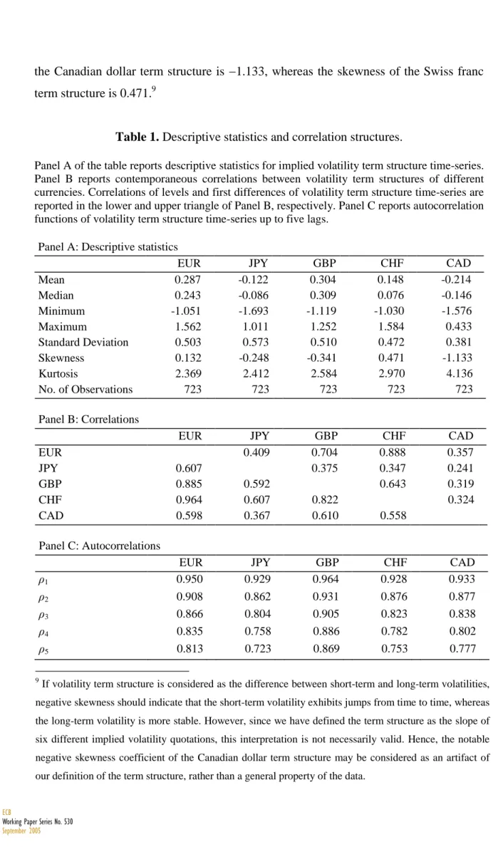
The term structure of implied volatilities is estimated for each currency on each trading day by fitting a linear model of at-the-money forward implied volatility as a function of time to maturity based on least squares criterion. Table 1 reports descriptive statistics of the estimated implied volatility term structure time-series. Several interesting features can be noted from this table. Perhaps the most prominent feature in Panel A is the difference between the volatility term structures of the European and non-European currencies. For the euro, British pound and Swiss franc, the implied volatilities of longer maturity options exceed, on average, the volatilities of shorter maturity options, while the implied volatilities of the Japanese yen and Canadian dollar appear to decrease with time to maturity.

The estimated term structures reported in Panel A are in units of volatility percentage points per year. Hence, the mean volatility term structure estimate of 0.287 for the euro, for instance, indicates that implied volatility of the euro increases, on average, by 0.287 volatility percentage points per a horizon of one year, or equivalently, about 0.024 percentage points per month. A simple t-test for means and the Wilcoxon signed ranks test for medians demonstrate that the upward sloping volatility term structures of the European currencies and the downward sloping term structures of the Japanese yen and Canadian dollar are statistically significant. However, the range of observations for all currencies is relatively large, suggesting that implied volatility term structures are varying considerably over time. In fact, the estimated volatility term structures for all currencies ranged from upward sloping to downward sloping during the sample period.

The standard deviations reported in Panel A suggest that the volatility term structure of the Canadian dollar is less variable and the term structure of the Japanese yen more variable than the term structures of the European currencies. An F-test for equality of variances confirms that these differences are statistically significant. It may also be noted from Table 1 that the skewness coefficients of the volatility term structure time-series vary considerably from currency to currency. For instance, the skewness of

the Canadian dollar term structure is −1.133, whereas the skewness of the Swiss franc term structure is 0.471.9

Table 1. Descriptive statistics and correlation structures.

Panel A of the table reports descriptive statistics for implied volatility term structure time-series. Panel B reports contemporaneous correlations between volatility term structures of different currencies. Correlations of levels and first differences of volatility term structure time-series are reported in the lower and upper triangle of Panel B, respectively. Panel C reports autocorrelation functions of volatility term structure time-series up to five lags.

Panel A: Descriptive statistics

EUR JPY GBP CHF CAD

Mean 0.287 -0.122 0.304 0.148 -0.214 Median 0.243 -0.086 0.309 0.076 -0.146 Minimum -1.051 -1.693 -1.119 -1.030 -1.576 Maximum 1.562 1.011 1.252 1.584 0.433 Standard Deviation 0.503 0.573 0.510 0.472 0.381 Skewness 0.132 -0.248 -0.341 0.471 -1.133 Kurtosis 2.369 2.412 2.584 2.970 4.136 No. of Observations 723 723 723 723 723 Panel B: Correlations

EUR JPY GBP CHF CAD

EUR 0.409 0.704 0.888 0.357 JPY 0.607 0.375 0.347 0.241 GBP 0.885 0.592 0.643 0.319 CHF 0.964 0.607 0.822 0.324 CAD 0.598 0.367 0.610 0.558 Panel C: Autocorrelations

EUR JPY GBP CHF CAD

ρ1 0.950 0.929 0.964 0.928 0.933 ρ2 0.908 0.862 0.931 0.876 0.877 ρ3 0.866 0.804 0.905 0.823 0.838 ρ4 0.835 0.758 0.886 0.782 0.802 ρ5 0.813 0.723 0.869 0.753 0.777 9

If volatility term structure is considered as the difference between short-term and long-term volatilities, negative skewness should indicate that the short-term volatility exhibits jumps from time to time, whereas the long-term volatility is more stable. However, since we have defined the term structure as the slope of six different implied volatility quotations, this interpretation is not necessarily valid. Hence, the notable negative skewness coefficient of the Canadian dollar term structure may be considered as an artifact of our definition of the term structure, rather than a general property of the data.

Contemporaneous correlations between the implied volatility term structure time-series are reported in Panel B of Table 1. The lower triangle of Panel B reports correlations in levels while the upper triangle reports correlations in first differences. All correlations in Panel B are positive and statistically highly significant, thereby indicating that the volatility term structures are closely linked across currencies. However, it may also be noted from Panel B that the volatility term structures of the European currencies are extremely highly correlated, whereas the term structures of the Japanese yen and Canadian dollar are somewhat less correlated with the European currencies and also with respect to each other.

Autocorrelation functions of implied volatility term structure time-series up to five lags are reported in Panel C of Table 1. The significance of autocorrelations is tested with the Ljung-Box Q-statistic. All time-series exhibit rather similar autocorrelation structures with statistically significant positive autocorrelation coefficients for one through five lags. This evidently demonstrates that the implied volatility term structure time-series are not white noise. The first order autocorrelations range from 0.93 to 0.96, suggesting that volatility term structures are mean reverting. A conventional measure of persistence of shocks, the ratio ln0.5/lnρ1, implies a mean half-life of shocks to the volatility term structure processes of about 10 to 17 trading days.

Table 2. Unit root tests.

The table reports Augmented Dickey-Fuller (ADF) and Phillips-Perron (PP) unit root tests without a time trend for the implied volatility term structure time-series. The lag length for the unit root tests is decided based on the Schwarz information criterion. The critical value for the tests at the 1 % significance level is –3.44.

ADF p-value PP p-value

EUR -4.288 0.001 -3.697 0.004

JPY -5.135 0.000 -4.789 0.000

GBP -3.670 0.005 -3.178 0.022

CHF -4.577 0.000 -4.593 0.000

In order to determine whether the implied volatility term structure time-series are stationary, the augmented Dickey-Fuller and Phillips-Perron unit root tests are conducted. The lag length used in the tests is decided based on the Schwartz information criterion. The results of the unit root tests are reported in Table 2. As can be seen from the table, the null of a unit root is soundly rejected for all five implied volatility term structure time-series

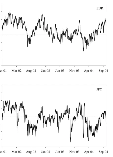
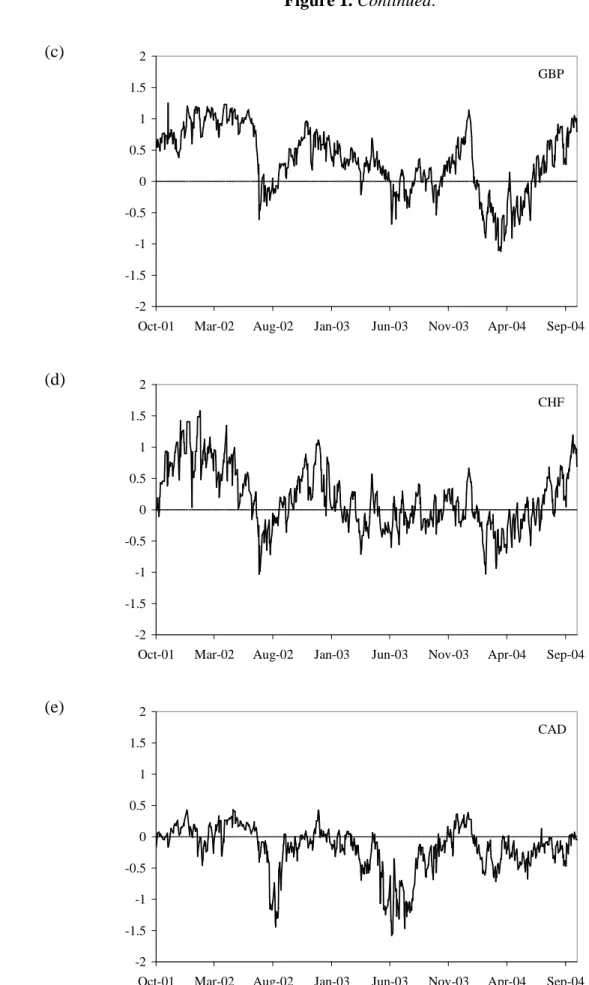
Developments of the estimated implied volatility term structures of the euro, Japanese yen, British pound, Swiss franc, and Canadian dollar over the period from October 2001 to September 2004 are plotted in Figures 1a−e. Several notable patterns emerge from these graphs. First, it is apparent that implied volatility term structures vary heavily over time. Although the descriptive statistics in Table 1 show that the volatility term structures of European currencies tend to be upward sloping, sustained periods of downward sloping term structures may also be observed from the graphs.

Moreover, Figures 1a−e indicate that implied volatility term structures may change substantially, and turn from upward sloping to downward sloping, in a short period of time. For instance, in June 2001 the slope of the British pound term structure wandered around unity until it suddenly dropped to –0.60 during the last trading days of June, and stayed mostly negative for the next 1½ months. These sudden shifts in the volatility term structure are also evident in the graphs of other currencies. As the descriptive statistics in Table 1 also suggest, the volatility term structure of the Canadian dollar seems considerably more stable and the term structure of Japanese yen more variable than the term structures of European currencies.

Finally, it can be noted from Figures 1a−e that implied volatility term structures exhibit somewhat similar patterns over time, thereby suggesting that some common factors may determine the time-varying behavior of volatility term structures across currencies. For instance, the volatility term structures of all currencies were mostly upward sloping from October 2001 until June 2002, and then, as already described above for the British pound, suddenly became downward sloping at the end of June. From July 2002 onwards, a moderate upward drift in the slopes of all volatility term structures may be observed from the graphs. Similarly, in December 2003 all implied volatility term structures were upward sloping and shifted to downward sloping very rapidly in January 2004. Finally, in the latter part of the sample period from spring 2004 onwards, the slopes of volatility term structures seem to exhibit a common upward

trend. Overall, Figures 1a−e together with the highly significant correlations reported in Table 1 suggest that implied volatility term structures are closely linked across currencies.

Figure 1. Implied volatility term structures.

(a) (b) -2 -1.5 -1 -0.5 0 0.5 1 1.5 2

Oct-01 Mar-02 Aug-02 Jan-03 Jun-03 Nov-03 Apr-04 Sep-04 EUR -2 -1.5 -1 -0.5 0 0.5 1 1.5 2

Oct-01 Mar-02 Aug-02 Jan-03 Jun-03 Nov-03 Apr-04 Sep-04 JPY

Figure 1. Continued. (c) (d) (e) -2 -1.5 -1 -0.5 0 0.5 1 1.5 2

Oct-01 Mar-02 Aug-02 Jan-03 Jun-03 Nov-03 Apr-04 Sep-04 GBP -2 -1.5 -1 -0.5 0 0.5 1 1.5 2

Oct-01 Mar-02 Aug-02 Jan-03 Jun-03 Nov-03 Apr-04 Sep-04 CHF -2 -1.5 -1 -0.5 0 0.5 1 1.5 2

Oct-01 Mar-02 Aug-02 Jan-03 Jun-03 Nov-03 Apr-04 Sep-04 CAD

4. Empirical findings

4.1. Common factors of implied volatility term structures

Given that implied volatility term structures, an individual term structure measured as the slope of the term structure, Xj,t, appear to be closely linked across currencies, it of interest to examine whether some k common factors {Ψ_p, p=1,2,…, k}

of first-differenced volatility term structure time-series {∆Xj,t} can be identified. In

order to determine the existence and the number of common factors affecting the movements in the term structures of implied volatilities, it is first assumed that the variance of changes in the term structure of any given currency can be decomposed into common variance and unique variance. Common variance is shared by movements of all volatility term structures included in the system, whereas unique variance is specific to a particular currency and also includes an error component. Within a linear framework, these assumptions lead to the following model with k common factors:

∑

where Xj,t denotes the implied volatility term structure for the jth currency, Ψp denotes the value of a common factor p, and the term αj,pΨp represents the contribution of the factor, εj,t denotes the residual error, and ∆ is the first difference operator.

The estimation results of the factor model given by Equation (1) are reported in Panel A of Table 3. The chi-square test statistic of 1941.5 with p-value<0.001 suggests

that the null hypothesis of no common factors can be soundly rejected. Hence, the test suggests that there is at least one common factor explaining the dynamics of implied volatility term structures across currencies. The chi-square statistic for the null hypothesis of the sufficiency of one common factor is 28.2 with p-value<0.001, thereby

indicating that more than one common factor may be required. By contrast, the hypothesis of no additional factors is not rejected. As can be seen from Panel A of Table 3, Akaike’s (AIC) and Schwarz’s (SIC) information criteria lead to the same conclusion as the chi-square test results. However, due to the relatively small number of term

structure time-series and based on the analysis of eigenvalues, a one-factor model may also be considered appropriate. Therefore, both one and two factor solutions for Equation (1) are presented in the following.

Panel A of Table 3 reports the one factor (FA1) and two factor (FA1, FA2) solutions of common factor analysis. The squared multiple correlation of a given first-differenced volatility term structure time-series with all the other term structure series in the system is used as a prior communality for each currency. The squared multiple correlations range from 0.149 for the volatility term structure of the Canadian dollar to 0.828 for euro, thereby indicating that the correlation of the volatility term structure of the Canadian dollar with all the other volatility term structures is substantially lower than the correlation of the euro. The squared correlation for the term structure of the Swiss franc is fairly close to that of the euro, while being somewhat lower for the volatility term structure of the British pound. The multiple squared correlation for the Japanese yen is 0.193, and thus the yen appears to correspond more closely to the Canadian dollar than to the European currencies. In brief, these findings imply that the volatility term structures of the European currencies are rather closely linked.

The estimation results for the one factor solution show that the factor loadings for the European currencies are all higher than 0.7. Moreover, they appear to be considerably higher than the loadings for the non-European currencies (0.418 for the yen and 0.317 for the Canadian dollar). The standardized regression coefficients show that the identified common factor makes by far the largest nonredundant individual contribution to the implied volatility term structure of the euro, with a standardized regression coefficient estimate of 0.820. The factor provides the second largest contribution to the volatility term structure of the Swiss franc, with a regression coefficient estimate equal to 0.139. Consequently, we interpret the identified common factor as a European factor. The squared multiple correlation of the implied volatility term structures with the European factor is 0.97. The identified factor accounts for 52 % of the total variance present among all time-series.

Table 3. Common factors and principal components.

The table reports Akaike’s (AIC) and Schwarz’s (SIC) information criteria and χ2 test statistic for the following null hypotheses: (i) no common factors (0), (ii) one factor is sufficient (1), and (iii) two factors are sufficient (2). Panel A reports common factor analysis of one (FA1) and two factor (FA1, FA2) solutions. Panel B reports principal component analysis of one (PC1) and two component (PC1, PC2) solutions. FAk and PCk denote loadings for the kth factor and principal component, respectively. The standardized regression coefficients for predicting the factors and the principal components from the first-differenced term structure time-series are denoted with SRC. The Prior column in Panel A reports the prior communalities of factor analysis, which are defined as the squared multiple correlation of a given first-differenced volatility term structure time-series with the other first-differenced term structure series in the system. The loadings for two common factors and principal components are based on VARIMAX rotation. The reported correlation is the squared multiple correlation of the variables with each factor. Explained variance is the variance explained by each factor ignoring the effects of all other factors.

Panel A. Common factors

Factors AIC SIC χ2 p-value

0 1941.5 0.000

1 18.27 -4.77 28.2 0.000

2 -1.32 -5.92 0.7 0.409

1-Factor solution 2-Factor solution

Currency Prior FA1 SRC FA1 SRC FA2 SRC

EUR 0.828 0.983 0.820 0.858 0.618 0.454 0.282 CHF 0.793 0.904 0.139 0.856 0.444 0.344 -0.295 GBP 0.513 0.719 0.042 0.548 -0.093 0.518 0.322 JPY 0.193 0.418 0.014 0.203 -0.152 0.519 0.339 CAD 0.149 0.371 0.012 0.224 -0.078 0.380 0.187 Correlation 0.97 0.81 0.44 Explained variance 0.52 0.37 0.20

Panel B. Principal components

1-Component solution 2-Component solution

Currency PC1 SRC PC1 SRC PC2 SRC EUR 0.966 0.772 0.704 0.906 0.223 -0.175 CHF 0.880 0.087 0.366 0.073 -0.239 -0.023 GBP 0.749 0.117 -0.104 0.069 0.332 0.032 JPY 0.446 0.043 -0.150 0.018 0.320 0.025 CAD 0.402 0.046 -0.086 -0.170 0.207 0.941 Correlation 0.95 0.81 0.43 Explained variance 0.53 0.37 0.20

The factor loadings for the two factor solution are based on an orthogonal VARIMAX rotation of the factor axes, in which the squared loadings of a factor on all the variables in a factor matrix are maximized.10 In a simple rotated solution, each factor has a small number of large loadings and a large number of small loadings, thereby simplifying the interpretation. The factor loadings of the first factor are higher than 0.5 for the volatility term structures of European currencies and are somewhat lower for the term structures of non-European currencies. The standardized regression coefficients for the volatility term structures of the euro and Swiss franc are 0.618 and 0.444, respectively, thereby suggesting that the first factor of this two factor specification closely corresponds to the identified factor in the one factor specification. Hence, we may again interpret the factor as the European factor. The squared multiple correlation of this factor with the volatility term structures is 0.81. In the two factor solution, the first factor accounts for 37 % of the total variance.

The factor loadings of the second factor are all higher than 0.3. These loadings are largest in the case of the yen, pound and euro, being 0.519, 0.518, and 0.454, respectively. The standardized regression coefficients for the volatility term structures of the yen, pound and euro are 0.339, 0.322, and 0.282, respectively. Hence, we may interpret this second factor to be related to trading volume. The squared multiple correlation of the volume factor with the volatility term structures is 0.44, and the factor constitutes about 20 % of the total variance. Together the two common factors account for 57 % of the total variance in the system. However, it may also be noted that these two factors appear to describe the dynamics of the European volatility term structures more adequately than the dynamics of the term structures of the Japanese yen and Canadian dollar volatilities.

As the next step, in order to extract the maximum portion of the variance present in the system with composite variables {F , p=1,2,…, k}, we replace the assumption _p

that the variance can be decomposed into common and unique variance by the assumption that the changes in the volatility term structure time-series are captured solely by total variance. Within our linear framework, this leads to the following principal component representation:

∑

where Xj,t is the implied volatility term structure for the jth currency, F denotes the p value of the pth principal component, and ∆ is the first difference operator.

Panel B of Table 3 presents the results of the one component (PC1) and two component (PC1, PC2) solutions for the principal component model given by Equation (2). Since the determination of an appropriate number of principal components is an empirical issue, the Kaiser criterion and the scree test are applied to ascertain the number of principal components. The Kaiser criterion and the analysis of eigenvalues suggest that a one principal component solution is the most appropriate choice. However, for comparison purposes, a two component solution is also reported in the following.

The one principal component solution shows that the component loadings for the volatility term structures of the European currencies are all higher than 0.7, while being substantially lower in the case of the Japanese yen and Canadian dollar. Hence, similarly to the common factor analysis, we interpret the identified principal component as a European factor. The estimated standardized regression coefficient for the euro is substantially above all the other coefficient estimates. The squared multiple correlation of the volatility term structures with the identified principal component is 0.95. As can be seen from Panel B, the principal component explains 53 % of the variance.

Analogously to the common factor analysis, the principal components of the two component solution are based on VARIMAX rotation. The loadings of the first principal component are higher than 0.3 for the volatility term structures of the euro and Swiss franc. Furthermore, the standardized regression coefficient indicates a strong positive relation between the composite variable and the euro. The squared multiple correlation of the first principal component with the volatility term structures is 0.81 and this principal component constitutes 37 % of the variance. The loadings of the second principal component are higher than 0.3 for the volatility term structures of the British pound and Japanese yen. The standardized regression coefficients indicate a negative relation of the second component with the volatility term structure of the euro and a strongly positive relation with the volatility term structure of the Canadian dollar. Consequently, we interpret this principal component to be related to trading volume.

The principal component explains 20 % of the total variance and the squared multiple correlation of this component with the volatility term structures is 0.43.

In brief, both the common factor and principal component analyses indicate that a large proportion of the variation in implied volatility term structures across currencies can be explained by two common factors. We interpret the identified factors as a European factor and a trading volume related factor. Of these two factors, the European factor appears to dominate, as it accounts for more than half of the variation among implied volatility term structure time-series. It should be noted, however, that the identified two factors describe the dynamics of the European volatility term structures more adequately than the dynamics of the term structures of the Japanese yen and Canadian dollar volatilities.

4.2. Innovation accounting and variance decompositions within a VAR framework

Given that implied volatility term structure time-series are stationary, vector autoregressive (VAR) modeling is applied to examine the cross-dynamics of implied volatility term structures. Hence, it is assumed that the dynamics of volatility term structures of the euro, Japanese yen, British pound, Swiss franc, Canadian dollar are described by the following VAR(p) model:

∑

where x_t =(X_EUR,t,X_JPY,t,X_GBP,t,X_CHF,t,X_CAD,t)´ is a covariance stationary 5×1 vector of volatility term structures Xt, αααα is a 5×1 vector of intercepts, {ΦΦΦΦi, i= 1, 2,…, p} is a

5×5 matrix of autoregressive coefficients, εεεεt is a 5×1 vector of random disturbances with

zero mean and positive definite covariance matrix, and p denotes the lag order of the system.

The determination of the appropriate number of lags used in the VAR is an empirical issue. Hence, we apply Akaike’s, Schwartz’s and Hannan-Quinn information criteria and Lütkepohl’s modified likelihood ratio test for the lag order selection. The results of the lag length criteria and the likelihood ratio test are reported in Table 4. As

can be seen from the table, the likelihood ratio test and Akaike’s criterion suggest setting p=3, while Schwartz’s and Hannan-Quinn information criteria suggest p=1 and

p=2, respectively. Since the Breusch-Godfrey LM test indicates significant serial

correlation in the residuals of a VAR(2) model, we augment the system with one additional lag. Model diagnostics suggest that this specification is adequate. Consequently, the number of lags used in the analysis is set equal to 3.

Table 4. Lag order selection for the VAR(p) model.

The table reports Akaike’s (AIC), Schwarz’s (SIC), and Hannan-Quinn (HQ) information criteria and Lütkepohl’s modified likelihood ratio (LR) test for the lag order selection.

Lag AIC SIC HQ LR

0 1.688 1.720 1.700 1 -6.746 -6.553 -6.671 6011.980 2 -6.844 -6.492 -6.708 118.380 3 -6.847 -6.334 -6.649 50.827 4 -6.827 -6.154 -6.567 34.673 5 -6.809 -5.976 -6.487 35.947 6 -6.767 -5.774 -6.383 19.018 7 -6.770 -5.617 -6.325 49.819 8 -6.732 -5.418 -6.225 21.379 9 -6.696 -5.222 -6.126 22.618 10 -6.669 -5.034 -6.037 28.458

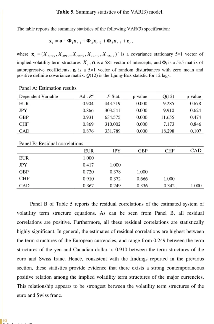
Panel A of Table 5 presents summary statistics of the VAR(3) estimation results. The F-statistic shows that the estimated model of implied volatility term structures is statistically highly significant with all p-values being less than 0.001. Moreover, the significance of the model is also shown in rather high R2s. The adjusted R2 is lowest for the Japanese yen (0.866) and highest for the British pound (0.931). Since the residuals of the VAR should exhibit no serial correlation if there are enough lags in the model, the residual serial correlations are analyzed to confirm the adequacy of the lag order. Based on the Ljung-Box statistics reported in Table 5, the null hypotheses of white noise cannot be rejected, thereby suggesting that the selected lag order is adequate.

Table 5. Summary statistics of the VAR(3) model.

The table reports the summary statistics of the following VAR(3) specification:

t t t t t α Φ x Φ x Φ x ε x = + 1 ₋1 + 2 ₋2 + 3 ₋3 + ,

where x_t =(X_EUR,t,X_JPY,t,X_GBP,t,X_CHF,t,X_CAD,t)´ is a covariance stationary 5×1 vector of implied volatility term structures X_t, αααα is a 5×1 vector of intercepts, and ΦΦΦΦi is a 5×5 matrix of autoregressive coefficients, εεεεt is a 5×1 vector of random disturbances with zero mean and positive definite covariance matrix. Q(12) is the Ljung-Box statistic for 12 lags.

Panel A: Estimation results

Dependent Variable Adj. R2 F-Stat. p-value Q(12) p-value

EUR 0.904 443.519 0.000 9.285 0.678 JPY 0.866 303.541 0.000 9.910 0.624 GBP 0.931 634.575 0.000 11.655 0.474 CHF 0.869 310.002 0.000 7.173 0.846 CAD 0.876 331.789 0.000 18.298 0.107

Panel B: Residual correlations

EUR JPY GBP CHF CAD

EUR 1.000

JPY 0.417 1.000

GBP 0.720 0.378 1.000

CHF 0.910 0.372 0.666 1.000

CAD 0.367 0.249 0.336 0.342 1.000

Panel B of Table 5 reports the residual correlations of the estimated system of volatility term structure equations. As can be seen from Panel B, all residual correlations are positive. Furthermore, all these residual correlations are statistically highly significant. In general, the estimates of residual correlations are highest between the term structures of the European currencies, and range from 0.249 between the term structures of the yen and Canadian dollar to 0.910 between the term structures of the euro and Swiss franc. Hence, consistent with the findings reported in the previous section, these statistics provide evidence that there exists a strong contemporaneous positive relation among the implied volatility term structures of the major currencies. This relationship appears to be strongest between the volatility term structures of the euro and Swiss franc.

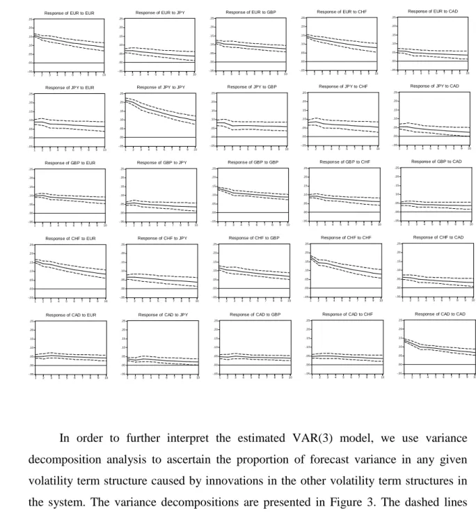
Impulse response analysis is used to examine the shock transmission mechanism between the variables in the estimated VAR(3) system. To avoid problems with the ordering of the variables in the system, the generalized impulses proposed by Pesaran and Shin (1998) are applied. Hence, the analysis is based on generalized one standard deviation shocks on the implied volatility term structures.

Figure 2 presents the impulse response functions of implied volatility term structures (indicated by the solid lines) and the Monte Carlo simulated 95 percent confidence intervals (indicated by the dashed lines) for the volatility term structures of the euro, Japanese yen, British pound, Swiss franc and Canadian dollar. The responses of the volatility term structures of the yen, British pound and Canadian dollar to a shock in the volatility term structure of the euro indicate that after the contemporaneous effect, the term structures still increase on the next day, while after that they start to decay except for the volatility term structure of the Canadian dollar, which appears to decay after the second day. A similar pattern may be observed for the impulse response of the volatility term structure of the Canadian dollar to a shock in the volatility term structure of the British pound. Interestingly, the impulse response functions indicate that the Swiss franc has the greatest influence on the euro among the currencies investigated. Given the analysis of common factors in the previous section, this finding further signifies that there exists a very strong linkage between the volatility term structures of the Swiss franc and the euro.

In sum, the analysis of the impulse response functions shows that a shock in the implied volatility term structure of the euro significantly affects the volatility term structures of all the other major currencies. A shock in the term structure of the euro affects the volatility term structures of the Japanese yen, British pound, Swiss franc and Canadian dollar contemporaneously, while the whole impact seems to be incorporated into the volatility term structures of the yen and British pound within two days and into the term structure of the Canadian dollar within three days. All the impulse responses decay after the third day, and thereby confirm that the system is stationary.

Figure 2. Impulse response functions.

The graphs present the impact of a generalized one standard deviation innovation in the implied volatility term structure of a given currency on itself and on the other implied volatility term structures in the system. Two standard error confidence intervals are presented around each impulse response function.

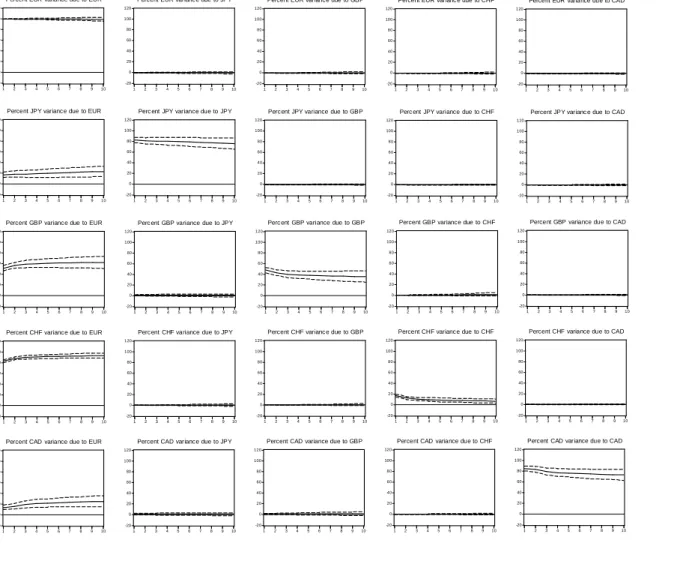
In order to further interpret the estimated VAR(3) model, we use variance decomposition analysis to ascertain the proportion of forecast variance in any given volatility term structure caused by innovations in the other volatility term structures in the system. The variance decompositions are presented in Figure 3. The dashed lines around each variance decomposition represent the 95 percent confidence intervals based on Monte Carlo simulation.

-.05 .00 .05 .10 .15 .20 .25 1 2 3 4 5 6 7 8 9 10

Response of EUR to EUR

-.05 .00 .05 .10 .15 .20 .25 1 2 3 4 5 6 7 8 9 10

Response of EUR to JPY

-.05 .00 .05 .10 .15 .20 .25 1 2 3 4 5 6 7 8 9 10 Response of EUR to GBP -.05 .00 .05 .10 .15 .20 .25 1 2 3 4 5 6 7 8 9 10 Response of EUR to CHF -.05 .00 .05 .10 .15 .20 .25 1 2 3 4 5 6 7 8 9 10

Response of EUR to CAD

-.05 .00 .05 .10 .15 .20 .25 1 2 3 4 5 6 7 8 9 10

Response of JPY to EUR

-.05 .00 .05 .10 .15 .20 .25 1 2 3 4 5 6 7 8 9 10

Response of JPY to JPY

-.05 .00 .05 .10 .15 .20 .25 1 2 3 4 5 6 7 8 9 10 Response of JPY to GBP -.05 .00 .05 .10 .15 .20 .25 1 2 3 4 5 6 7 8 9 10 Response of JPY to CHF -.05 .00 .05 .10 .15 .20 .25 1 2 3 4 5 6 7 8 9 10

Response of JPY to CAD

-.05 .00 .05 .10 .15 .20 .25 1 2 3 4 5 6 7 8 9 10 Response of GBP to EUR -.05 .00 .05 .10 .15 .20 .25 1 2 3 4 5 6 7 8 9 10 Response of GBP to JPY -.05 .00 .05 .10 .15 .20 .25 1 2 3 4 5 6 7 8 9 10 Response of GBP to GBP -.05 .00 .05 .10 .15 .20 .25 1 2 3 4 5 6 7 8 9 10 Response of GB P to CHF -.05 .00 .05 .10 .15 .20 .25 1 2 3 4 5 6 7 8 9 10 Response of GBP to CAD -.05 .00 .05 .10 .15 .20 .25 1 2 3 4 5 6 7 8 9 10 Response of CHF to EUR -.05 .00 .05 .10 .15 .20 .25 1 2 3 4 5 6 7 8 9 10 Response of CHF to JPY -.05 .00 .05 .10 .15 .20 .25 1 2 3 4 5 6 7 8 9 10 Response of CHF to GBP -.05 .00 .05 .10 .15 .20 .25 1 2 3 4 5 6 7 8 9 10 Response of CHF to CHF -.05 .00 .05 .10 .15 .20 .25 1 2 3 4 5 6 7 8 9 10 Response of CHF to CAD -.05 .00 .05 .10 .15 .20 .25 1 2 3 4 5 6 7 8 9 10

Response of CAD to EUR

-.05 .00 .05 .10 .15 .20 .25 1 2 3 4 5 6 7 8 9 10

Response of CAD to JPY

-.05 .00 .05 .10 .15 .20 .25 1 2 3 4 5 6 7 8 9 10 Response of CAD to GBP -.05 .00 .05 .10 .15 .20 .25 1 2 3 4 5 6 7 8 9 10 Response of CAD to CHF -.05 .00 .05 .10 .15 .20 .25 1 2 3 4 5 6 7 8 9 10

Figure 3. Variance decompositions.

The graphs present the percentage of forecast variance of the implied volatility term structure of a given currency caused by innovations in itself and in the other implied volatility term structures in the system. Two standard error confidence intervals are presented around each variance decomposition.

Figure 3 shows that virtually all of the forecast variance of the implied volatility term structure of the euro is caused by its own innovations, thereby indicating that the volatility term structures of the other major currencies do not have any significant impact on the volatility term structure of the euro. By contrast, the implied volatility term structure of the euro seems to have a substantial impact on the volatility term structures of all other major currencies.

The term structure of the euro explains approximately 19 % of the two days ahead and about 24 % of the ten days ahead forecast error variance of the yen, and about 57 %

-20 0 20 40 60 80 100 120 1 2 3 4 5 6 7 8 9 10

Percent EUR variance due to EUR

-20 0 20 40 60 80 100 120 1 2 3 4 5 6 7 8 9 10

Percent EUR variance due to JPY

-20 0 20 40 60 80 100 120 1 2 3 4 5 6 7 8 9 10

Percent EUR variance due to GBP

-20 0 20 40 60 80 100 120 1 2 3 4 5 6 7 8 9 10

Percent EUR varianc e due to CHF

-20 0 20 40 60 80 100 120 1 2 3 4 5 6 7 8 9 10

Percent EUR variance due to CAD

-20 0 20 40 60 80 100 120 1 2 3 4 5 6 7 8 9 10

Percent JPY variance due to EUR

-20 0 20 40 60 80 100 120 1 2 3 4 5 6 7 8 9 10

Perc ent JPY variance due to JPY

-20 0 20 40 60 80 100 120 1 2 3 4 5 6 7 8 9 10

Percent JPY variance due to GBP

-20 0 20 40 60 80 100 120 1 2 3 4 5 6 7 8 9 10

Perc ent JPY variance due to CHF

-20 0 20 40 60 80 100 120 1 2 3 4 5 6 7 8 9 10

Percent JPY varianc e due to CAD

-20 0 20 40 60 80 100 120 1 2 3 4 5 6 7 8 9 10

Percent GBP variance due to EUR

-20 0 20 40 60 80 100 120 1 2 3 4 5 6 7 8 9 10

Perc ent GBP variance due to JPY

-20 0 20 40 60 80 100 120 1 2 3 4 5 6 7 8 9 10

Perc ent GBP variance due to GBP

-20 0 20 40 60 80 100 120 1 2 3 4 5 6 7 8 9 10

Percent GBP variance due to CHF

-20 0 20 40 60 80 100 120 1 2 3 4 5 6 7 8 9 10

Percent GBP variance due to CAD

-20 0 20 40 60 80 100 120 1 2 3 4 5 6 7 8 9 10

Percent CHF variance due to EUR

-20 0 20 40 60 80 100 120 1 2 3 4 5 6 7 8 9 10

Percent CHF variance due to JPY

-20 0 20 40 60 80 100 120 1 2 3 4 5 6 7 8 9 10

Percent CHF varianc e due to GBP

-20 0 20 40 60 80 100 120 1 2 3 4 5 6 7 8 9 10

Percent CHF variance due to CHF

-20 0 20 40 60 80 100 120 1 2 3 4 5 6 7 8 9 10

Percent CHF variance due to CAD

-20 0 20 40 60 80 100 120 1 2 3 4 5 6 7 8 9 10

Percent CAD variance due to EUR

-20 0 20 40 60 80 100 120 1 2 3 4 5 6 7 8 9 10

Percent CAD variance due to JPY

-20 0 20 40 60 80 100 120 1 2 3 4 5 6 7 8 9 10

Percent CAD variance due to GBP

-20 0 20 40 60 80 100 120 1 2 3 4 5 6 7 8 9 10

Percent CAD variance due to CHF

-20 0 20 40 60 80 100 120 1 2 3 4 5 6 7 8 9 10

and 62 % of the two and ten days ahead forecast errors of variance of the pound, respectively. The term structure of the euro explains preponderance of the two days

ahead (88 %) and ten days ahead (93 %) forecast error variance of the Swiss franc. Together with the preceding analysis, this finding demonstrates that there exists a rather deviant relationship between the implied volatility term structures of the euro and Swiss franc. For the volatility term structure of the Canadian dollar, the corresponding figures are 16 % and 25 %, respectively. In brief, the variance decompositions indicate that the

term structures of implied volatilities of the Japanese yen, British pound, Swiss franc, and Canadian dollar are significantly affected by the implied volatility term structure of the euro. With respect to the European currencies, the results indicate that a vast proportion of the forecast error variances of the British pound and Swiss franc may be explained by the volatility term structure of the euro.

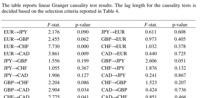
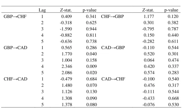
4.3. Linear and nonlinear causality

Given the preceding analysis, it is of interest to examine whether any causal dynamics are present among the implied volatility term structure time-series. For this purpose, we use linear and nonlinear Granger causality tests. For the general formalization of causality in the case of two stationary volatility term structure time-series {X,t} and {Y,t}, we consider the conditional distribution function F(Xt It−1). Define two information sets It-1 consisting of the lagged vectors of X with lag lengths Lx

and Y with lag lengths Ly. The first information set I0,t-1={ Xt-Lx Lx } includes a lag

vector of X and the second information set I1,t-1={ Xt-LxLx; Yt-LyLy } includes lag vectors

of X and Y. Using the following notation for m-length lead vectors of X, Xmt ={Xt, ...

Xt+m-1}, and Lx -length lag vector of X and Ly -length lag vector of Y, Xt-LxLx ={Xt-Lx, ...

Xt-1} and Yt-Ly Ly ={Yt-Ly, ... Yt-1}, respectively, the time-series {Yt} does not strictly

Granger cause {Xt} for given lags Lx and Ly and for any arbitrary t if:

) (

)

(X_t I_0,t−1 =F X_t I_1,t−1

In practice, the estimation of distributional functions is impeded due to the limited number of observations. Consequently, as proposed by Granger (1969), the mean squared error (MSE) of the optimal linear predictor of Xt is considered in the

following. The definition (4) of the absence of Granger causality can hence be formulated as: ) ( ) (Xt I0,t−1 =MSE Xt I1,t−1 MSE . (5)

As proposed by Baeck and Brock (1992) and Hiemstra and Jones (1994), the implication of strict Granger noncausality for two strictly stationary and weakly dependent time-series {Xt} and {Yt} can be defined as follows. Consider the probability

) (⋅

P of two m-length lead vectors of X being in the ε-distance from each other conditional to the ε-distance closeness of lag-vectors of X and lag-vectors of Y. Using

the previous notation, time-series {Yt} does not strictly Granger cause {Xt} for given

values of m, Lx, Ly and ε if:

(

)

(

)

where the maximum norm a =maxiai is used as a measure of the spatial distance between the vectors. The absence of causality means that for two arbitrary time points t

and s, the probability of lead vectors of X being in the ε-distance from each other, conditional to the ε-neighbourhood of the lags vector of X, does not depend on whether

the lag vectors of Y are in the ε-distance from each other.

Replacing the conditional probabilities by the ratios of joint probabilities

( )

(

) ( )

P = ∩ / and substituting { X_tm_−Lx+Lx −X_sm₋+_LxLx <ε} for { Xt X

m s m − <ε, Xt Lx X Lx s Lx Lx

− − − <ε}, the Granger noncausality conditions given by Equation (6) can be

P X X Y Y P X X Y Y P X X P X X t Lx m Lx s Lx m Lx t Ly Ly s Ly Ly t Lx Lx s Lx Lx t Ly Ly s Ly Ly t Lx m Lx s Lx m Lx t Lx Lx s Lx Lx ( , ) ( , ( ) ( ) −+ −+ − − − − − − −+ −+ − − − < − < − < − < = − < − < ε ε ε ε ε ε . (7)

This strict Granger noncausality can then be expressed as:

) , ( 4 ) , ( 3 ) , , ( 2 ) , , ( 1 ε ε εε P Lx Lx m P Ly Lx P Ly Lx m P + = + . (8)

Linear Granger causality can be tested by the standard joint Wald test within the VAR framework. Consider a bivariate representation of the VAR(p) model given by

Equation (3) , where _      = t t t Y X x and _       = ) ( ) ( ) ( ) ( ) ( _{21 22} 12 11 p p p p p i i i i i Φ Φ Φ Φ

Φ _{. The null hypothesis}

that time-series {Yt} does not strictly Granger cause {Xt} is rejected if the coefficients in

) ( 12

p

i

Φ _{are jointly significantly different from zero. If both} 12_(p)

i

Φ _and 21_(p)

i

Φ _are

non-zero, bidirectional causality is present. The feasibility of the Granger causality test depends on the stationarity features of the time-series in the system.11

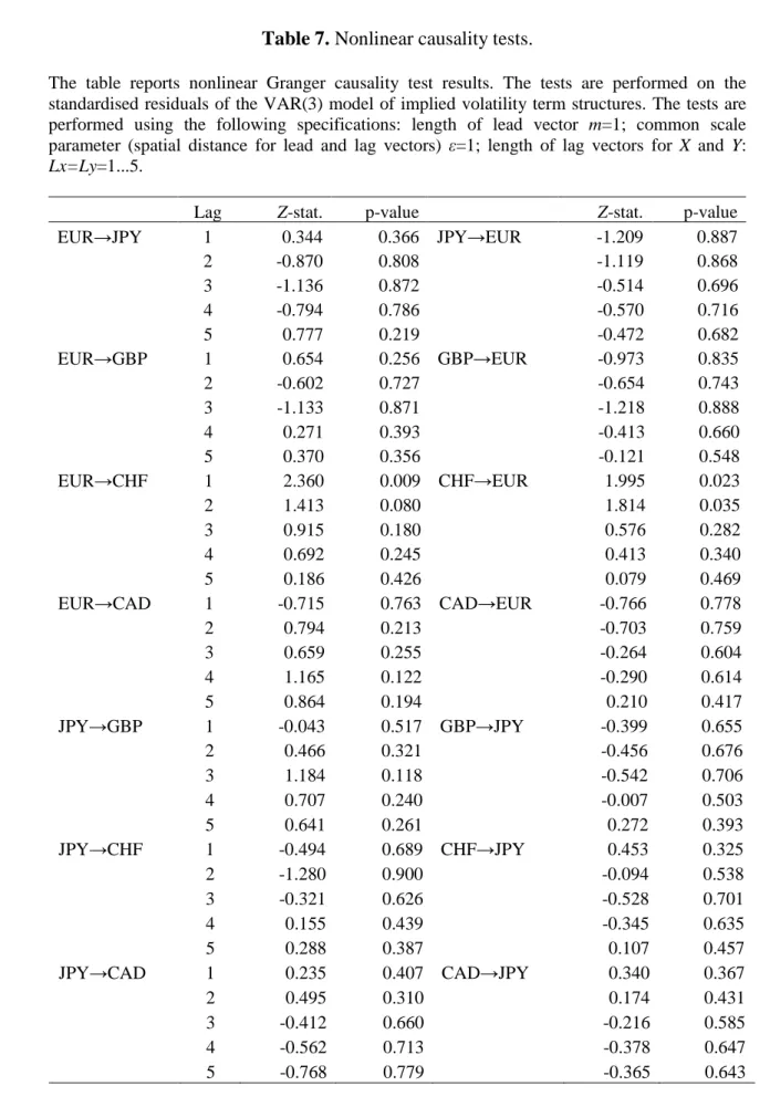
In order to examine whether nonlinear causality is present in the system of implied volatility term structures, we apply a modified version of the Baeck and Brock (1992) nonparametric test for nonlinear Granger causality proposed by Hiemstra and Jones (1994). Appendix 1 provides a more detailed description of this test. The nonlinear causality test presumes that the time-series are not linearly dependent. Therefore, to ensure that linear causality is first eliminated from the system, the nonlinear causality test is performed on the residuals of the VAR(3) model summarized in Table 5.

11 _{Toda and Philips (1993) demonstrate that the distribution of the Wald statistics becomes non-standard}