Mean Shift Based Clustering in High Dimensions: A Texture Classification Example

Mean Shift Based Clustering in High Dimensions:

A Texture Classification Example

Bogdan Georgescu

Ilan Shimshoni

Peter Meer

Computer Science

Industrial Engineering and Management

Electrical and Computer Engineering

Technion - Israel Institute of Technology

Rutgers University, Piscataway, NJ 08854, USA

Haifa 32000, ISRAEL

georgesc, [email protected]

[email protected]

Abstract

Feature space analysis is the main module in many com-puter vision tasks. The most popular technique, k-means clustering, however, has two inherent limitations: the clus-ters are constrained to be spherically symmetric and their number has to be known a priori. In nonparametric clus-tering methods, like the one based on mean shift, these limitations are eliminated but the amount of computation becomes prohibitively large as the dimension of the space increases. We exploit a recently proposed approximation technique, locality-sensitive hashing (LSH), to reduce the computational complexity of adaptive mean shift. In our implementation of LSH the optimal parameters of the data structure are determined by a pilot learning procedure, and the partitions are data driven. As an application, the per-formance of mode and k-means based textons are compared in a texture classification study.

1. Introduction

Representation of visual information through feature space analysis received renewed interest in recent years, moti-vated by content based image retrieval applications. The increase in the available computational power allows today the handling of feature spaces which are high dimensional and contain millions of data points.

The structure of high dimensional spaces, however, de-fies our three dimensional geometric intuition. Such spaces are extremely sparse with the data points far away from each other [17, Sec.4.5.1]. Thus, to infer about the local struc-ture of the space only a small number of data points may be available, which can yield erroneous results. The

phe-nomenon is known in the statistical literature as thecurse of

dimensionality, and its effect increases exponentially with the dimension. The curse of dimensionality can be avoided only by imposing a fully parametric model over the data [6, p.203], an approach which is not feasible for a high dimen-sional feature space with a complex structure.

The goal of feature space analysis is to reduce the data to a few significant features through a procedure known

un-der many different names, clustering, unsupervised learn-ing, or vector quantization. Most often different variants ofk-means clusteringare employed, in which the feature space is represented as a mixture of normal distributions [6,

Sec.10.4.3]. The number of mixture components is

usu-ally set by the user.

The popularity of the k-means algorithm is due to its

low computational complexity of , whereis the

number of data points,the dimension of the space, and

the number of iterations which is always small relative to.

However, since it imposes a rigid delineation over the fea-ture space and requires a reasonable guess for the number of clusters present, the k-means clustering can return erro-neous results when the embedded assumptions are not satis-fied. Moreover, the k-means algorithm is not robust, points

which do not belong to any of the clusters can move the

estimated means away from the densest regions.

A robust clustering technique which does not require prior knowledge of the number of clusters, and does not

constrain the shape of the clusters, is themean shiftbased

clustering. This is also an iterative technique, but instead of the means, it estimates the modes of the multivariate distri-bution underlying the feature space. The number of clusters is obtained automatically by finding the centers of the dens-est regions in the space (the modes). See [1] for details. Un-der its original implementation the mean shift based cluster-ing cannot be used in high dimensional spaces. Already for

, in a video sequence segmentation application, a

fine-to-coarse hierarchical approach had to be introduced [5]. The most expensive operation of the mean shift method is finding the closest neighbors of a point in the space. The

problem is known in computational geometry as

multidi-mensional range searching [4, Chap.5]. The goal of the range searching algorithms is to represent the data in a structure in which proximity relations can be determined

in less than time. One of the most popular

struc-tures, the kD-tree, is built in operations, where

the proportionality constant increases with the dimension of the space. A query selects the points within a rectangu-lar region delimited by an interval on each coordinate axis,

and the query time for kD-trees has complexity bounded by

½

, where is the number of points found.

Thus, for high dimensions the complexity of a query is

prac-tically linear, yielding thecomputational curse of

dimen-sionality. Recently, several probabilistic algorithms have been proposed for approximate nearest neighbor search. The algorithms yield sublinear complexity with a speedup which depends on the desired accuracy [7, 10, 11].

In this paper we have adapted the algorithm in [7] for mean shift based clustering in high dimensions. Work-ing with data in high dimensions also required that we ex-tend the adaptive mean shift procedure introduced in [2]. All computer vision applications of mean shift until now, such as image segmentation, object recognition and track-ing, were in relatively low-dimensional spaces. Our imple-mentation opens the door to use mean shift in tasks based on high-dimensional features.

In Section 2 we present a short review of the adaptive mean-shift technique. Locality-sensitive hashing, the tech-nique for approximate nearest neighbor search is described in Section 3, where we have also introduced refinements to handle data with complex structure. In Section 4 the per-formance of adaptive mean shift (AMS) in high dimensions is investigated, and in Section 5 AMS is used for texture classification based on textons.

2. Adaptive Mean Shift

Here we only review some of the results described in [2] which should be consulted for the details.

Assume that each data pointÜ

, is

associated with a bandwidth value . The sample

pointestimator Ü ÜÜ (1)

based on a spherically symmetric kernel with bounded

support satisfying

Ü Ü

Ü (2)

is an adaptive nonparametric estimator of the density at

lo-cationÜin the feature space. The function , ,

is called theprofileof the kernel, and the normalization

con-stant assures that Üintegrates to one. The function

can always be defined when the derivative

of the kernel profile exists. Using as the profile,

the kernelÜ is defined as Ü

Ü

.

By taking the gradient of (1) the following property can be proven Ñ Ü Ü Ü (3)

whereis a positive constant and

Ñ Ü ·¾ Ü Ü Ü ·¾ Ü Ü Ü (4)

is called themean shift vector. The expression (3) shows

that at locationÜthe weighted mean of the data points

se-lected with kernelis proportional to the normalized

den-sity gradient estimate obtained with kernel. The mean

shift vector thus points toward the direction of maximum increase in the density. The implication of the mean shift property is that the iterative procedure

Ý Ü ·¾ Ý Ü ·¾ Ý Ü (5)

is a hill climbing technique to the nearest stationary point of the density, i.e., a point in which the density gradient vanishes. The initial position of the kernel, the starting point

of the procedureÝ

can be chosen as one of the data points

Ü. Most often the points of convergence of the iterative

procedure are the modes (local maxima) of the density. There are numerous methods described in the

statisti-cal literature to define , the bandwidth values associated

with the data points, most of which use a pilot density es-timate [17, Sec.5.3.1]. The simplest way to obtain the pilot density estimate is by nearest neighbors [6, Sec.4.5]. Let

Ü

be the -nearest neighbor of the point

Ü. Then, we take Ü Ü (6) where

norm is used since it is the most suitable for the

data structure to be introduced in the next section. The choice of the norm does not have a major effect on the

per-formance. The number of neighbors should be chosen

large enough to assure that there is an increase in density

within the support of most kernels having bandwidths .

While the value of should increase withthe dimension

of the feature space, the dependence is not critical for the performance of the mean shift procedure, as will be seen

in Section 4. When all , i.e., a single global

band-width value is used, the adaptive mean shift (AMS) pro-cedure becomes the fixed bandwidth mean shift (MS) dis-cussed in [1].

A robust nonparametric clustering of the data is achieved by applying the mean shift procedure to a representative subset of the data points. After convergence, the detected modes are the cluster centers, and the shape of the clusters is determined by the basins of attraction. See [1] for details.

3. Locality-Sensitive Hashing

The bottleneck of mean shift in high dimensions is the need for a fast algorithm to perform neighborhood queries when computing (5). The problem has been addressed before in the vision community by sorting the data according to each

of the coordinates [13], but a significant speedup was

achieved only when the data is close to a low-dimensional manifold.

Recently new algorithms using tools from probabilistic approximation theory were suggested for performing ap-proximate nearest neighbor search in high dimensions for general datasets [10, 11] and for clustering data [9, 14]. We use the approximate nearest neighbor algorithm based on

locality-sensitive hashing(LSH) [7] and adapted it to han-dle the complex data met in computer vision applications. In a task of estimating the pose of articulated objects, de-scribed in these proceedings [16], the LSH technique was extended to accommodate distances in the parameter space.

3.1. High Dimensional Neighborhood Queries

Givenpoints in

the mean shift iterations (5) require

a neighborhood query around the current locationÝ . The

naive method is to scan the whole dataset and test whether

the kernel of the pointÜ coversÝ . Thus, for each mean

computation the complexity is . Assuming that for

every point in the dataset this operation is performed

times (a value which depends on the ’s and the

distribu-tion of the data), the complexity of the mean shift algorithm

is

.

To improve the efficiency of the neighborhood queries the following data structure is constructed. The data is

tes-sellatedtimes with random partitions, each defined by

inequalities (Figure 1). In each partitionpairs of random

numbers,

and

are used. First

, an integer between 1

andis chosen, followed by

, a value within the range of

the data along the

-th coordinate.

The pair

partitions the data according to the

in-equality (7) where

is the selected coordinate for the data point

Ü. Thus, for each point Ü each partition yields a

-dimensional boolean vector (inequality true/false). Points which have the same vector lie in the same cell of the parti-tion. Using a hash function, all the points belonging to the same cell are placed in the same bucket of a hash table. As

we havesuch partitions, each point belongs

simultane-ously tocells (hash table buckets).

To find the neighborhood of radius around a query

point,boolean vectors are computed using (7). These

vectors indexcells

,

in the hash table.

The points in their union

are the ones returned

by the query (Figure 1). Note that anyin the intersection

will return the same result. Thus

deter-mines the resolution of the data structure, whereas

termines the set of the points returned by the query. The

de-scribed technique is calledlocality-sensitive hashing(LSH)

and was introduced in [10].

Points close in

have a higher probability for collision

in the hash table. Since

lies close to the center of

,

the query will return most of the nearest neighbors of. The

example in Figure 1 illustrates the approximate nature of the

query. Parts of an

neighborhood centered on

are not

covered by

which has a different shape. The

approxima-tion errors can be reduced by building data structures with

larger

’s, however, this will increase the running time of

a query.

L

Figure 1: The locality-sensitive hashing data structure. For

the query pointthe overlap ofcells yields the region

which approximates the desired neighborhood.

3.2. Optimal Selection of

and

The values foranddetermine the expected volumes of

and

. The average number of inequalities used for

each coordinate is , partitioning the data into

regions. The average number of points

in a cell and in their union is (8)

Note that in estimating

we disregard that the points

belong to several

’s.

Qualitatively, the larger the value for, the number of

cuts in a partition, the smaller the average volume of the

cells

. Similarly, as the number of partitions

increases,

the volume of

decreases and of

given, only values of below a certain bound are of

interest. Indeed, onceexceeds this bound all the

neigh-borhood of radius aroundhas been already covered by

. Thus, larger values of

will only increase the query

time with no improvement in the quality of the results.

The optimal values ofandcan be derived from the

data. A subset of data pointsÜ , is

selected by random sampling. For each of these data points,

the

distance (6) to its k-nearest neighbor is

deter-mined accurately by the traditional linear algorithm. In the approximate nearest neighbor algorithm based on

LSH, for any pair of and, we define for each of the

points

, the distance to the k-nearest neighbor re-turned by the query. When the query does not return the

correct k-nearest neighbors

. The total running

time of the queries is . The optimal is

then chosen such that

(9) subject to:

whereis the LSH approximation threshold set by the user.

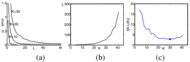
The optimization is performed as a numerical search

pro-cedure. For a givenwe compute, as a function of, the

approximation error of thequeries. This is shown in

Fig-ure 2a for a thirteen-dimensional real data set. By

thresh-olding the family of graphs at , the function

is obtained (Figure 2b). The running time can now be

ex-pressed as , i.e., a one-dimensional function in

, the number of employed cuts (Figure 2c). Its minimum

is

which together with

are the optimal

pa-rameters of the LSH data structure.

0 20 40 60 0 0.5 1 1.5 L error K=30 K=20 K=10 0 10 20 30 40 0 100 200 300 400 K L 0 10 20 30 40 0 5 10 15 20 K t[K,L(K)] (a) (b) (c)

Figure 2: Determining the optimal and. (a)

Depen-dence of the approximation error onfor .

The curves are thresholded at , dashed line. (b)

Dependence ofonfor . (c) The running time

. The minimum is marked ‘ ’.

The family of error curves can be efficiently generated.

The number of partitions is bounded by the available

computer memory. Let

be that bound. Similarly,

we can set a maximum on the number of cuts,

.

Next, the LSH data structure is built with

.

Then, the approximation error is computed incrementally

for

by adding one partition at a time.

This yields

which is subsequently used as

for

, etc.

3.3. Data Driven Partitions

The strategy of generating therandom tessellations has an

important influence on the performance of locality-sensitive

hashing. In [7] the coordinates

have equal chance to be

selected and the values

are uniformly distributed over

the range of the corresponding coordinate. This partitioning strategy works well only when the density of the data is ap-proximately uniform in the entire space. However, feature spaces associated with vision applications are often multi-modal. In [10, 11] the problem of nonuniformly distributed data was dealt with by building several data structures with

different values ofandto accommodate the different

local densities. The query is performed first under the as-sumption of a high density, and when it fails it is repeated for lower densities. The process terminates when the near-est neighbors are found.

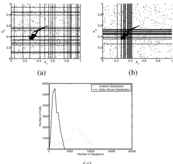
Our approach is to sample according to the marginal

dis-tributions along each coordinate. We use a few pointsÜ

chosen at random from the data set. For each point one of its coordinates is selected at random to define a cut. Using more than one coordinate from a point would imply sam-pling from partial joint densities, but does not seem to be more advantageous. Our adaptive, data driven strategy as-sures that in denser regions more cuts will be made yielding smaller cells, while in sparser regions there will be less cuts. On average all cells will contain a similar number of points. The two-dimensional data in Figure 3b and 3b comprised of four clusters and uniformly distributed background, is used to demonstrate the two sampling strategies. In both cases the same number of cuts were used but the data driven method places most of the cuts over the clusters (Figure 3b). For a quantitative performance assessment a data set of ten normal distributions with arbitrary shapes (5000 points each) were defined in 50 dimensions. When the data driven strategy is used, the distribution of the number of points in a cell is much more compact and their average value is much lower (Figure 3c). As a consequence, the data driven strategy yields more efficient k-nearest neighbor queries for complex data sets.

4. Mean Shift in High Dimensions

Given Ý , the current location in the iterations, an LSH

based query retrieves the approximate set of neighbors needed to compute the next location (5). The resolution of the data analysis is controlled by the user. In the fixed bandwidth MS method the user provides the bandwidth

0 0.2 0.4 0.6 0.8 1 0 0.2 0.4 0.6 0.8 1 X₁ X2 0 0.2 0.4 0.6 0.8 1 0 0.2 0.4 0.6 0.8 1 X₁ X2 (a) (b) 0 5000 10000 15000 20000 0 1000 2000 3000 4000 5000 6000 Number of Neighbors Number of Cells Uniform Distribution Data−Driven Distribution (c)

Figure 3: Uniform vs. data driven partitions. Typical re-sult for two-dimensional data obtained with (a) uniform; (b) data driven strategy. (c) Distribution of points-per-cell for a 50-dimensional data set.

of neighbors used in the pilot density procedure. The

pa-rametersandof the LSH data structure are selected

em-ploying the technique discussed in Section 3.2. The

band-widths associated with the data points are obtained by

performingneighborhood queries. Once the bandwidths

are set, the adaptive mean shift procedure runs at approx-imately the same cost as the fixed bandwidth mean shift. Thus, the difference between MS and AMS is only one ad-ditional query per point.

An ad-hoc procedure provides further speedup. Since

the resolution of the data structure is

, with high

prob-ability one can assume that all the points within

will

converge to the same mode. Thus, once any point from a

is associated with a mode, the subsequent queries to

automatically return this mode and the mean shift iterations stop. The modes are stored in a separate hash table whose

keys are theboolean vectors associated with

.

4.1. Adaptive vs. Fixed Bandwidth Mean Shift

generated. From these , points belonged to ten

spherical normal distributions (clusters) whose means were positioned on a line through the origin. The standard devi-ation increases as the mean becomes more distant from the origin. For an adjacent pair of clusters, the ratio of the sum of standard deviations to the distance between the means was kept constant. The remaining 100,000 points were uni-formly distributed in the 50-dimensional cube. Plotting the

distances of the data points from the origin yields a graph very similar to the one in Figure 4a. Note that the points farther from the origin have a larger spread.

The performance of the fixed bandwidth (MS) and the adaptive mean shift (AMS) procedures is compared for var-ious parameter values in Figure 4. The experiments were performed for 500 points chosen at random from each clus-ter, a total of 5000 points. The location associated with each

selected point after the mean shift procedure, is the

em-ployed performance measure. Ideally this location should be near the center of the cluster to which the point belongs.

In the MS strategy, when the bandwidth is small, due

to the sparseness of the high-dimensional space very few

points have neighbors within distance . The mean shift

procedure does not start and the allocation of the points is to

themselves (Figure 4a). On the other hand as increases the

windows become too large for some of the local structures and points may converge incorrectly to the center (mode) of an adjacent cluster (Figures 4b to 4d).

The pilot density estimation in the AMS strategy auto-matically adapts the bandwidth to the local structure. The parameter , the number of neighbors used for the pilot es-timation does not have a strong influence. The data is

pro-cessed correctly for to 500, except for a few points

(Figures 4e to 4g), and even for only some of the

points in the cluster with the largest spread converge to the adjacent mode (Figure 4h). The superiority of the adaptive mean shift in high dimensions is clearly visible. Due to the sparseness of the 50-dimensional space, the 100,000 points in the background did not interfere with the mean shift pro-cesses under either strategy, proving its robustness.

The use of the LSH data structure in the mean shift pro-cedure assures a significant speedup. We have derived four different features spaces from a texture image with the filter banks discussed in the next section. The spaces had

dimen-sionand 48, and containedpoints.

An AMS procedure was run both with linear and approxi-mate queries for 1638 points. The number of neighbors in

the pilot density estimation was . The

approxima-tion error of the LSH was . The running times (in

seconds) in Table 1 show the achieved speedups.

Table 1: Running Times of AMS Implementations

Traditional LSH Speedup

4 1,507 80 18.8

8 1,888 206 9.2

13 2,546 110 23.1

48 5,877 276 21.3

The speedup will increase with the number of data points

, and will decrease with the number of neighbors .

There-fore in the mean shift procedure the speedup is not as high as in applications in which only a small number of neigh-bors are required.

0 1000 2000 3000 4000 5000 1 1.2 1.4 1.6 1.8 2 2.2 2.4 2.6 2.8 3x 10 5 h=100 Points Distance 0 1000 2000 3000 4000 5000 1 1.2 1.4 1.6 1.8 2 2.2 2.4 2.6 2.8 3x 10 5 h=1400 Points Distance 0 1000 2000 3000 4000 5000 1 1.2 1.4 1.6 1.8 2 2.2 2.4 2.6 2.8 3x 10 5 h=2700 Points Distance 0 1000 2000 3000 4000 5000 1 1.2 1.4 1.6 1.8 2 2.2 2.4 2.6 2.8 3x 10 5 h=4000 Points Distance (a) (b) (c) (d) 0 1000 2000 3000 4000 5000 1 1.2 1.4 1.6 1.8 2 2.2 2.4 2.6 2.8 3x 10 5 k=100 Points Distance 0 1000 2000 3000 4000 5000 1 1.2 1.4 1.6 1.8 2 2.2 2.4 2.6 2.8 3x 10 5 k=300 Points Distance 0 1000 2000 3000 4000 5000 1 1.2 1.4 1.6 1.8 2 2.2 2.4 2.6 2.8 3x 10 5 k=500 Points Distance 0 1000 2000 3000 4000 5000 1 1.2 1.4 1.6 1.8 2 2.2 2.4 2.6 2.8 3x 10 5 k=700 Points Distance (e) (f) (g) (h)

Figure 4: Distance from the origin of 5000 points from ten 50-dimensional clustersafterfixed bandwidth mean shift (MS):

(a) to (d); and adaptive mean shift (AMS) : (e) to (h). The parameters: MS – bandwidth ; AMS – number of neighbors .

5. Texture Classification

Efficient methods exist for texture classification under vary-ing illumination and viewvary-ing direction [3],[12], [15], [18]. In the state-of-the-art approaches a texture is characterized

throughtextons, which are cluster centers in a feature space

derived from the input. Following [12] this feature space is built from the output of a filter bank applied at every pixel. However, as was shown recently [19], neighborhood infor-mation in the spatial domain may also suffice.

The approaches differ in the employed filter bank.

– LM: A combination of 48 anisotropic and isotropic

fil-ters were used by Leung and Malik [12] and Cula and Dana [3]. The filters are Gaussian masks, their first derivative and Laplacian, defined at three scales. Be-cause of the oriented filters, the representation is sen-sitive to texture rotations. The feature space is 48 di-mensional.

– S: A set of 13 circular symmetric filters was used by

Schmid [15] to obtain a rotationally invariant feature set. The feature space is 13 dimensional.

– M4, M8: Both representations were proposed by

Varma and Zissermann [18]. The first one (M4) is based on 2 rotationally symmetric and 12 oriented fil-ters. The second set is an extension of the first one at 3 different scales. The feature vector is computed by retaining only the maximum response for the oriented filters (2 out of 12 for M4 and 6 out of 36 for M8), thus reducing the dependence on the global texture orienta-tion. The feature space is 4 respectively 8 dimensional. To find the textons, usually the standard k-means clus-tering algorithm is used, which as was discussed in

Sec-tion 1 has several limitaSec-tions. The shape of the clusters is restricted to be spherical and their number has to be set prior to the processing.

The most significant textons are aggregated into the

tex-ton library. This serves as a dictionary of representative local structural features and must be general enough to char-acterize a large variety of texture classes. A texture is then

modeled through its texton histogram. The histogram is

computed by defining at every pixel a feature vector, re-placing it with the closest texton from the library (vector quantization) and accumulating the results over the entire image.

Let two textures and be characterized by the

his-tograms and built from textons. As in [12] the

distance between these two texton distributions

(10) is used to measure similarity, although note the absence of

the factorto take into account that the comparison is

be-tweentwohistograms derived from data. In a texture

clas-sification task the training image with the smallest distance from the test image determines the class of the latter.

In our experiments we substituted the k-means based clustering module with the adaptive mean shift (AMS) based robust nonparametric clustering. Thus, the textons

instead of beingmean basedare nowmode based, and the

number of the significant ones is determined automatically. The complete Brodatz database containing 112 textures with varying degrees of complexity was used in the experi-ments. Classification of the Brodatz database is challenging

because it contains many nonhomogeneous textures. The

images were divided into four

subim-ages with half of the subimsubim-ages being used for training (224 models) and the other half for testing (224 queries). The normalizations recommended in [18] (both in the image and filter domains) were also performed.

The number of significant textons detected with the AMS procedure depends on the texture. We have limited the num-ber of mode textons extracted from a texture class to five. The same number was used for the mean textons. Thus, by adding the textons to the library, a texton histogram has at

most bins.

Table 2: Classification Results for the Brodatz Database

Filter M4 M8 S LM

RND 84.82% 88.39% 89.73% 92.41%

k-means 85.71% 94.64% 93.30% 97.32%

AMS 85.27% 93.75% 93.30% 98.66%

The classification results using the different filter banks are presented in Table 2. The best result was obtained with the LM mode textons, an additional three correct classifica-tions out of the six errors with the mean textons. However, there is no clear advantage in using the mode textons with the other filter banks.

The classification performance is close to its upper bound defined by the texture inhomogeneity, due to which the test and training images of a class can be very different. This observation is supported by the performance degrada-tion obtained when the database images were divided into

sixteen subimages and the same half/half partition

yielded 896 models and 896 queries. The recognition rate decreased for all the filter banks. The best result of 94%, was again obtained with the LM filters for both the mean and mode textons. In [8], with the same setup but employ-ing a different texture representation, and usemploy-ing only 109 textures from the Brodatz database the recognition rate was

.

A texture class is characterized by the histogram of the textons, an approximation of the feature space distribution. The histogram is constructed from a Voronoi diagram with

cells. The vertices of the diagram are the textons, and

each histogram bin contains the number of feature points in a cell. Thus, variations in textons translate in approximat-ing the distribution by a different diagram, but it appears to have a weak influence on the classification performance. When by uniform sampling five random vectors were cho-sen as textons, the classification performance (RND) de-creased only between 1% to 6%.

The k-means clustering imposes rigidly a given number of identical spherical clusters over the feature space. Thus, it is expected that when this structure is not adequate, the mode based textons will provide a more meaningful decom-position of the texture image. This is proven in the

follow-5 10 15 20 0 0.2 0.4 0.6 0.8 1 Texton No. Percentage

texture classified pixels

mode mean

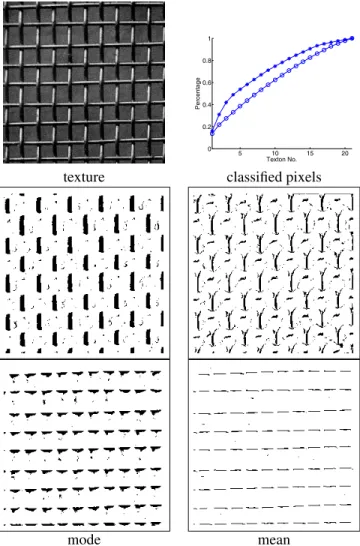
Figure 5: Mode ( ) vs. mean (Æ) based textons. The

lo-cal structure is better captured by the mode textons. D001 texture, LM filter bank.

ing two examples.

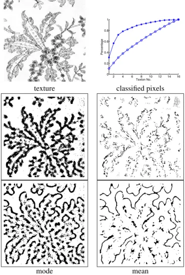
In Figure 5 the LM filter bank was applied to a regular texture. The AMS procedure extracted 21 textons, the num-ber also used in the k-means clustering. However, when ordered by size, the first few mode textons are associated with more pixels in the image than the mean textons, which always account for a similar number of pixels. The differ-ence between the mode and mean textons can be seen by marking the pixels associated with textons of the same lo-cal structure (Figure 5, bottom). The advantage of the mode based representation is more evident for the nonregular tex-ture in Figure 6, where the cumulative distribution of the mode textons classified pixels is has a sharper increase.

Since textons capture local spatial configurations, we be-lieve that combining the mode textons with the representa-tion proposed in [19] can offer more insight into why the texton approach is superior to previous techniques.

2 4 6 8 10 12 14 16 0 0.2 0.4 0.6 0.8 1 Texton No. Percentage

texture classified pixels

mode mean

Figure 6: Mode ( ) vs. mean (Æ) based textons. The

lo-cal structure is better captured by the mode textons. D040 texture, S filter bank.

6. Conclusion

We have introduced a computationally efficient method that makes possible in high dimensional spaces the detection of the modes of distributions. By employing a data structure based on locality-sensitive hashing, a significant decrease in the running time was obtained while maintaining the qual-ity of the results. The new implementation of the mean shift procedure opens the door to the development of vision algo-rithms exploiting feature space analysis – including learning techniques – in high dimensions. The C++ source code of this implememtation of mean shift can be downloaded from

http://www.caip.rutgers.edu/riul .

Acknowledgments

We thank Bogdan Matei of the Sarnoff Corporation, Prince-ton, NJ, for calling our attention to the LSH data structure. This work was done during the sabbatical of I.S. at Rutgers University. The support of the National Science Foundation under the grant IRI 99-87695 is gratefully acknowledged.

References

[1] D. Comaniciu and P. Meer. Mean shift: A robust approach toward feature space analysis. IEEE Trans. Pattern Anal. Machine Intell., 24(5):603–619, 2002.

[2] D. Comaniciu, V. Ramesh, and P. Meer. The variable band-width mean shift and data-driven scale selection. InProc. 8th Intl. Conf. on Computer Vision,Vancouver, Canada, vol-ume I, pages 438–445, July 2001.

[3] O. G. Cula and K. J. Dana. Compact representation of bidi-rectional texture functions. InProc. IEEE Conf. on Computer Vision and Pattern Recognition,Kauai, Hawaii, volume 1, pages 1041–1047, 2001.

[4] M. de Berg, M. van Kreveld, M. Overmars, and O. Schwartzkopf.Computational Geometry. Algorithms and Applications. Springer, second edition, 1998.

[5] D. DeMenthon. Spatio-temporal segmentation of video by hierarchical mean shift analysis. InProc. Statistical Meth-ods in Video Processing Workshop,Copenhagen, Denmark, 2002. Also CAR-TR-978 Center for Automat. Res., U. of Md, College Park.

[6] R.O. Duda, P.E. Hart, and D.G. Stork.Pattern Classification. Wiley, second edition, 2001.

[7] A. Gionis, P. Indyk, and R. Motwani. Similarity search in high dimensions via hashing. InProc. Int. Conf. on Very Large Data Bases, pages 518–529, 1999.

[8] G. M. Haley and B. S. Manjunath. Rotation-invariant tex-ture classification using a complete space-frequency model. IEEE Trans. Image Process., 8(2):255–269, 1999.

[9] P. Indyk. A sublinear time approximation scheme for clus-tering in metric spaces. InProc. IEEE Symp. on Foundations of Computer Science, pages 154–159, 1999.

[10] P. Indyk and R. Motwani. Approximate nearest neighbors: towards removing the curse of dimensionality. In Proc. Symp. on Theory of Computing, pages 604–613, 1998. [11] E. Kushilevitz, R. Ostrovsky, and Y. Rabani. Efficient

search for approximate nearest neighbor in high dimensional spaces. InProc. Symp. on Theory of Computing, pages 614– 623, 1998.

[12] T. Leung and J. Malik. Representing and recognizing the visual appearance of materials using three-dimensional tex-tons.Intl. J. of Computer Vision, 43(1):29–44, 2001. [13] S.A. Nene and S.K. Nayar. A simple algorithm for

nearest-neighbor search in high dimensions. IEEE Trans. Pattern Anal. Machine Intell., 19(9):989–1003, 1997.

[14] R. Ostrovsky and Y. Rabani. Polynomial time approximation schemes for geometric k-clustering. InProc. IEEE Symp. on Foundations of Computer Science, pages 349–358, 2000. [15] C. Schmid. Constructing models for content-based image

re-trieval. InProc. IEEE Conf. on Computer Vision and Pattern Recognition,Kauai, Hawaii, volume 2, pages 39–45, 2001. [16] G. Shakhnarovich, P. Viola, and T. Darrell. Fast pose

esti-mation with parameter-sensitive hashing. InProc. 9th Intl. Conf. on Computer Vision,Nice, France, 2003.

[17] B. W. Silverman.Density Estimation for Statistics and Data Analysis. Chapman & Hall, 1986.

[18] M. Varma and A. Zisserman. Classifying images of materi-als. InProc. European Conf. on Computer Vision, Copen-hagen, Denmark, volume III, pages 255–271, 2002. [19] M. Varma and A. Zisserman. Texture classification: Are

filter banks necessary? InProc. IEEE Conf. on Computer Vision and Pattern Recognition,Madison, Wisconsin, vol-ume II, pages 691–698, 2003.