Optimization of Nonpoint Source Best Management Practices Selection
through a Calibrated HSPF Modeling Approach
Joshua Charles Hunn
A thesis submitted to the faculty of the University of North Carolina at Chapel Hill in
partial fulfillment of the requirements for the degree of Master of Science in the
Department of Environmental Sciences and Engineering
Chapel Hill
2007
Approved by:
ABSTRACT
JOSHUA HUNN: Optimization of Nonpoint Source Best Management Practices
Selection through a Calibrated HSPF Modeling Approach
(Under the direction of Gregory W. Characklis)
ACKNOWLEDGEMENTS
I would like to acknowledge all those at the University of North Carolina, and
particularly the Department of Environmental Sciences and Engineering, who contributed
to my education and my development throughout these past two years. I feel that the
lessons that I have learned here will lead well beyond the classroom and will serve me
well wherever the future might take me. I want to particularly recognize my advisor, Dr.
Greg Characklis, for his constant support and assistance throughout the whole process.
I want to thank my family and friends, both past and present, who have supported
me, not only for these past two years, but throughout my whole life. Your
CONTENTS
Page
LIST
OF
TABLES
vii
LIST
OF
FIGURES
ix
LIST OF ABBREVIATIONS AND SYMBOLS
xi
Chapter
I
INTRODUCTION
1
1.1
Regulatory
Background
2
1.2
Study
Significance
2
1.3 Effects of Nonpoint Source Pollution
3
1.4 Nonpoint Source Characterization
4
1.4.1 Microbial Source Trends
4
1.4.2 Nonpoint Source Modeling
5
1.4.3 Model Selection
6
1.5 Nonpoint Source Pollution Controls
7
II
METHODS
9
2.1 Watershed Characterization
9
2.2 Weather Data Preparation
10
2.3 HSPF Model Development
11
2.3.1 PERLND Theory Development
11
2.3.2 IMPLND Theory Development
14
2.3.3 HSPF Parameter Development
16
2.4 Parameter Calibration
16
2.4.1
Data
Inventory
17
2.4.2 Hydrology Calibration
17
2.4.3 Fecal Coliform Calibration
19
2.6 BMP Analysis Framework
21
III
RESULTS
25
3.1
Model
Validation
25
3.2 Regulatory Violation Validation
27
3.3 Source Loading Identification
29
3.4 Nonpoint Source Controls
30
3.4.1 Source Control Examination
31
3.4.2 BMP Optimization Results
33
3.4.3 BMP Costs
34
APPENDICES
A.
Spatial Representation of Northeast Creek Watershed
38
B.
BASINS watershed characterization and subwatershed delineation
40
C.
Weather
Data
Preparation
41
D.
HSPF
PERLND
Module
Processes
47
E.
HSPF IMPLND Module Processes
56
F.
HSPF PERLND Accumulation Rate Development
60
G.
HSPF
Input
Parameters
62
H.
HSPF
Code
64
I.
Calibration
Data
106
J.
Error
Quantification
109
K.
BMP
Characteristics
113
L.
Source
Loading
Characterization
114
M. BMP Linear Optimization Model
115
N. BMP Optimization Model Sensitivity Analysis
133
O. Assessment of BMP Costs
135
LIST OF TABLES
Table
Page
1. Summary of BMP characteristics that were used in the
optimization analysis (full compilation of sources
found in Appendix K)
24
2.
Summary of in-stream and effluent FC concentrations
for the period of January 1, 2005 - June 30, 2006
29
3.
Lowest cost strategy of urban land coverage in each
subwatershed whose runoff must be intercepted by
stormwater
wetlands
33
4.
Summary of costs associated with management practices
for the control of FC in Northeast Creek watershed
34
B.1. Allocation of land use by subwatershed
40
C.1. Hourly distribution coefficients for wind speed
43
C.2. Summary of weather input parameters and processing in
WDMUtil required for HSPF modeling
46
F.1. Population of agricultural animals in Northeast Creek
watershed along with their respective fecal coliform
production
rates
60
F.2. Wildlife population densities in the forest land cover, as
well as their respective fecal coliform production rates
61
F.3. Fecal coliform production rates for urban land cover, as well as
the fraction of the urban land cover associated with each use
61
G.1. Summary of HSPF input parameters
62
I.1. Summary of in-stream FC data used for calibration and
Verification
106
K.1. Summary of BMP efficiencies
113
O.1. Table displaying the population growth that would be
expected over the next 20 years, as well as verifying
that a contribution of $57/person/year would be
LIST OF FIGURES
Figure
Page
1. Schematic of possible nonpoint sources of pollution into
a water
body
1
2. Spatial representation of Northeast Creek watershed
8
3.
Northeast Creek subwatershed delineation with
corresponding
reach
numbers
10
4. Representation of the hydrological flow process for the
PERLND module in HSPF
11
5. Modeled flow at Reach 11 vs. observed USGS gauge flow data
18
6. Comparison of Modeled vs. Observed in-stream FC
concentrations for (a) Reach 5 and (b) Reach 3
during
calibration
19
7. Cumulative monthly rainfall and modeled FC contributions
from
Subwatershed
1
26
8a-b. Comparison of Modeled vs. Observed in-stream FC
concentrations for (a) Reach 5 and (b) Reach 3 during
validation
26
9. Modeled in-stream 5-day running geometric mean concentration
at locations above (Reach 3) and below (Reach 5) the
Triangle Wastewater Treatment Plant
28
10. Relative fractions of sources of in-stream fecal coliform loading
30
11a-b. Comparison of source reduction control strategies with baseline
conditions for locations (a) above and (b) below the WWTP
32
12. Modeled in-stream running 5-day geometric mean FC
concentrations following implementation of least cost
BMP
allocation
scenario
34
A.1. Placement of Northeast Creek watershed within the Piedmont
A.2. Placement of Northeast Creek watershed within the Haw
River Subbasin and the Cape Fear River Basin
39
C.1. Spatial locations of four data sources for hourly
precipitation as retrieved from the State Climate
Office
of
North
Carolina
45
D.1. Structural representation of the PERLND module
within
HSPF
47
D.2a-b. Flow diagram of water movement and storage as
modeled in the PWAT section of the PERLND
module
in
HSPF
48
D.3. Flow diagram for sediment processes in the HSPF
PERLND
module
54
D.4. Flow diagram for quality constituent processes in the
HSPF
PERLND
module
55
E.1. Structural chart for the IMPLND module of HSPF
56
E.2. Flow model for the hydrological processes associated
with the IMPLND module in HSPF
57
E.3. Flow model for the solids processes associated with the
IMPLND
module
in
HSPF
58
E.4. Flow model for the quality constituent processes associated
with the IMPLND module in HSPF
59
J.1a-b. Comparison of observed vs. modeled in-stream
concentrations of fecal coliform for the calibration period
of January 1,2001-December 31, 2001 with order of
magnitude boundaries for (a) Reach 5 and (b) Reach 3
110
J.2a-b. Comparison of observed vs. modeled in-stream
concentrations of fecal coliform for validation period of
January 1, 2002-December 31, 2002 with order of
magnitude boundaries for (a) Reach 5 and (b) Reach 3
112
L.1. Relative fraction of FC loading as attributable to each of
the pervious land surface areas, with wetlands and forest land
LIST OF ABBREVIATIONS
Abbreviations
ac
:
acre
ATEM
:
air
temperature
AWND
: average daily wind speed
BASINS
: Better Assessment Science Integrating Point and Nonpoint
Sources
BIT
:
Bacterial
Indicator
Tool
BMP
: best management practice
cfs
: cubic feet per second
CFU
: colony forming units
CLOU
:
cloud
cover
cm
:
centimeter
CWA
: Clean Water Act
DCLO
: daily percent cloud cover
DEM
: digital elevation model
DEVT
: daily potential evapotranspiration
DEWP
: hourly dewpoint temperature
DPTP
: daily dewpoint temperature
EVAP
:
potential
evaporation
FC
:
fecal
coliform
HSPF
: Hydrological Simulation Program-FORTRAN
IMPLND
: impervious land segments
NC
:
North
Carolina
NHD
:
National
Hydrography
Dataset
NCDC
: National Climatic Data Center
NPDES
: National Pollutant Discharge Elimination System
PERLND
: pervious land segments
PEVT
:
potential
evapotranspiration
PQUAL
: HSPF module describing fecal coliform movement and storage
PREC
:
precipitation
PSUN
:
percent
sun
PWAT
: HSPF module describing water flow and storage
RCHRES
: free-flowing reaches or mixed reservoir
RDU
:
Raleigh-Durham
Airport
SCONC
: State Climate Office of North Carolina
SOLR
:
solar
radiation
sq km
: square kilometer
TMAX
:
maximum
temperature
TMDL
: Total Maximum Daily Load
TMIN
:
minimum
temperature
USEPA
: United States Environmental Protection Agency
WIND
:
wind
speed
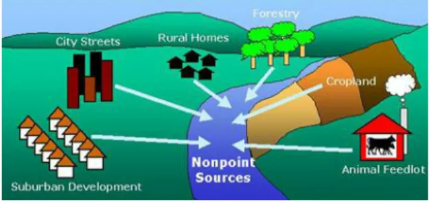
Figure 1: Schematic of possible nonpoint sources of pollution into a water body (NOAA 2006).
Chapter I
Introduction
The passage of the landmark Clean Water Act (CWA) sought to ensure that all
water bodies would be “fishable and swimmable” by requiring identification of, and
remediation plans for, water bodies deemed physically, biologically or chemically
impaired. However, thirty-five years later, more than 40% of assessed water bodies still
do not comply with applicable water quality standards (USEPA 2007d). Substantial
improvements in water quality have occurred through the control of point source
discharges, primarily accomplished through the creation of the National Pollutant
Discharge Elimination System (NPDES) program (USEPA 2007b). Effective point
source controls have only shifted responsibility, however, as nonpoint sources are now
the primary cause of surface water
impairments (USEPA 1996), thereby
necessitating greater understanding and
action (USGAO 1990). Nonpoint sources
(Figure 1) primarily include overland
runoff from pervious and impervious land,
selection will be critically important to the development of effective water quality
improvement strategies (Lehner et al. 1999).
1.1 Regulatory Background
Under the CWA, each state is tasked with identifying water bodies that do not
meet federal or state mandated used-based water quality standards. For each impaired
water body, the state must determine a pollutant-specific total maximum daily load
(TMDL)
1that the impaired water body can receive from all sources (both point and
nonpoint) while maintaining regulatory compliance (USEPA 1972b). These impaired
water bodies, placed on a state-generated 303(d) list (a number referencing the relevant
section of the CWA), have been given priority status in terms of regulating point source
discharges. When point source controls alone are insufficient to achieve compliance,
consideration of nonpoint sources is required (USEPA 1972a). This latter provision of
the CWA was largely ignored, however, until citizen groups brought lawsuits in the late
1990’s pressuring the Environmental Protection Agency into action (USEPA 2007d).
These suits were settled largely in favor of citizen groups, forcing the USEPA and
individual states to accelerate the rate at which impaired waters were identified and
brought into compliance.
1.2 Study Significance
Currently, more than 20,000 water body segments have been identified as
impaired for at least one pollutant of concern (USEPA 2007d), such that nearly
three-quarters of the population of the United States live within ten miles of an impaired water
body. However, this number is likely far greater given that nationally only 19% of all
river and streams have been assessed (SFWMD 2007). Of those water bodies that have
been assessed, pathogens are the primary cause of more than 40% of North Carolina’s
and 13% of the United States’ total in-stream impairments
2(USEPA 2007a; USEPA
2007c), which underscores the importance of work addressing this issue. Unfortunately
for the policy process, nonpoint source monitoring for a water body, particularly when
microbially impaired, is generally cost-prohibitive, meaning that a comprehensive
description of overland sources and their magnitudes is often impossible. Rather, many
regulatory decisions are supported by water quality models which address this problem
from a watershed scale. Given that most impaired water bodies have received minimal
attention regarding the development of comprehensive plan to ensure and maintain
regulatory compliance, this report offers a method for integrating the selection of
microbial nonpoint source pollution controls into the TMDL policy framework using a
representative watershed.
1.3 Effects of Nonpoint Source Pollution
Fecal coliforms are indicator organisms that serve as surrogates for human enteric
pathogens such as Shigella, Salmonella, Giardia, and Cryptosporidium that are more
difficult and costly to detect (Olivieri 1982; Bohn and Buckhouse 1985; Schueller 1999).
Large-scale disease outbreaks attributable to these pathogens have occurred in public
drinking water supplies, including those in Milwaukee (MacKenzie et al. 1994), Clark
County, Nevada (Goldstein et al. 1996), and western Georgia (Hayes et al. 1989). Other
studies have concluded that health risks also exist from recreational contact with
biologically-impaired surface waters, particularly those that receive significant
stormwater runoff (Pruss 1998; Haile et al. 1999; Curriero et al. 2001; Dwight et al. 2004;
Stoner and Dorfman 2006).
Improvements made in surface water quality will alleviate the potential for illness
from contact with impaired water bodies. Studies have shown that though the costs of
managing and improving stormwater runoff can be high, the costs associated with
post-treatment waterborne illnesses can potentially be much greater (Corso et al. 2003;
Gaffield et al. 2003). This advocates for a preemptive approach to managing the public
health effects associated with microbial contaminants in surface waters. In addition, from
a development standpoint, research has shown that property values can actually increase
for lots that are situated near certain stormwater controls, though this assumes that proper
upkeep and maintenance is performed (Emmerling-DiNovo 1995; USEPA 1995).
1.4 Nonpoint Source Characterization
The loading of nonpoint source pollution to surface waters is highly variable,
depending upon a number of factors that have been considered in the development and
modification of comprehensive nonpoint pollution models (Loague et al. 1998).
1.4.1 Microbial Source Trends
well to land use patterns, with both agricultural and urban residential land cover typically
having the highest bacterial loading rates (Francy et al. 2000; Arienzo et al. 2001; Tong
and Chen 2002; Tufford and Marshall 2002; Kelsey et al. 2004; Mehaffey et al. 2005;
Schoonover et al. 2005). Elevated contributions from urban areas have also been closely
linked to increases in housing density and impervious land cover (Bannerman et al. 1993;
Young and Thackston 1999; Mallin et al. 2000; Mallin et al. 2001). Principally, fecal
coliform sources include direct deposition by wildlife, failing septic systems, and
surcharging or failing sanitary sewers (Petersen 2005), though, because of the
watershed-specific characteristics that determine fecal coliform loads, bacterial source tracking has
been developed to better identify precise sources (Wiggins et al. 1999; Dombek et al.
2000; Burnes 2003). Finally, in-stream bacterial concentrations are also seen to vary
seasonally, with summer months generally displaying higher levels (Van Donsel et al.
1967; Geldreich et al. 1968; Edwards et al. 1997).
1.4.2 Nonpoint Source Modeling
concentrations as a function of physical parameters (Brezonik and Stadelmann 2002) or
probabilistic models (Behera et al. 2006), though either was difficult to calibrate and
validate. In an effort to increase confidence, computer-based nonpoint source pollution
models have evolved to incorporate these loading characteristics with the capacity for the
incorporation of localized physical parameters (Donigan Jr. and Huber 1991). Even
though initial pollutant modeling efforts were targeted solely toward nitrogen,
phosphorous, and sediment, further model efforts have included microbial constituents
(Ferguson et al. 2003; Arnold and Fohrer 2005), though with no explicit consideration of
bacteria-sediment interactions
3.
1.4.3 Model Selection
The Hydrological Simulation Program-FORTRAN (HSPF) code was selected to
model this system and can be described in terms of several general characteristics:
•
It is continuous, which allows for long-term trends to be modeled, rather
than simply a single storm event;
•
It is deterministic, such that an identical output will be achieved for every
run completed with identical inputs;
•
It is lumped parameter, which simplifies the model to allow localized
parameters to be given the same value; and
•
It is defined in terms of the watershed, which ensures
hydrologically-consistent boundaries on the analysis (Center 2006).
•
The HSPF code has been used in the development of several bacterial
TMDLs (Yagow et al. 2001; Moyer and Hyer 2003; USEPA 2003;
Benham et al. 2005; Benham et al. 2006), providing useful background for
this modeling effort.
3
1.5 Nonpoint Source Pollution Controls
Nonpoint sources, due to their diffuse nature, are more difficult to control and are
managed through a variety of best management practices (BMPs). A BMP can take one
of two forms: (i) structural, meaning that controls are instituted to reduce pollutant loads
after they have already been mobilized within the watershed through the use of hardware
to alter flow paths, residence times, or infiltration capacity, or (ii) non-structural, which
seek to prevent or reduce pollutant loads at the source without the use of any hardware
(USEPA 1999). Examples of structural BMPs include wet or dry detention ponds,
stormwater wetlands, buffer strips, grassed swales, and bioretention, while non-structural
BMPs include redirected runoff, street sweeping, wildlife exclusion and educational
programs (USEPA 2005b). This report suggests an approach to the selection of BMP
control strategies for microbial contaminants using a linear programming framework that
minimizes costs while ensuring regulatory compliance through integration with a fully
calibrated and validated nonpoint source pollution model.
1.6 Study Location
Northeast Creek, which resides within a watershed located in the Piedmont region
of North Carolina (Figure 2, with more detail in Appendix A), contains a 15.8-kilometer
segment that is biologically impaired based on elevated fecal coliform (FC)
Figure 2: Spatial representation of Northeast Creek watershed.
Chapter II
Methods
HSPF requires user input of physical and chemical parameters to model
watershed hydrology, suspended solids, and general quality constituents (in this case,
fecal coliforms). The processes outlined below are used to develop, calibrate and
validate an HSPF model integrating point and nonpoint source contributions. Model
output will be used as input to a proposed optimization model for nonpoint source control
selection to develop a least-cost strategy for achieving regulatory compliance.
2.1 Watershed Characterization
The HSPF model requires several inputs: (i) a watershed map file; (ii) a
hydrographic reach file; (iii) assignation of land cover, and; (iv) regional climatic data.
The first three inputs were developed using the Better Assessment Science Integrating
Point and Nonpoint Sources (BASINS) modeling framework, which serves as a
preprocessor for several nonpoint source models (USEPA 2001).
6
8
2
4 1
3
7 5
9
10
11
Figure 3: Northeast Creek subwatershed delineation with corresponding reach numbers.
identifying those water bodies and their corresponding overland flow planes which drain
into Northeast Creek. Subwatersheds were automatically generated
4corresponding to the
major tributaries (Burdens Creek, Kit Creek,
and Panther Creek) and their associated
overland, interflow, and groundwater flow
planes (Figure 3).
While the DEM and NHD that were
accessed through BASINS were sufficient
for the scope of this project, the land cover
dataset was outdated, and more recent data
were acquired through the USGS
5(2004).
ArcGIS tools were then used to determine
the amount of land cover that existed within
each subwatershed (Appendix B).
2.2 Weather Data Preparation
A climatic dataset was developed for the watershed which primarily includes
temperature and rainfall. For HSPF, all datasets are compiled and displayed in WDMUtil
(Hummel et al. 2001), an external processor that will also organize outputted data.
Following a procedure developed by the Virginia Tech Center for TMDL and Watershed
Studies (Zeckoski 2006), most of the weather data was acquired from the National
4In addition to the automatic subwatershed delineation in BASINS, an additional outlet was manually added corresponding to the location of a USGS stream gage (at Reach 11) from which in-stream flow measurements were obtained. This also accounts for the reason that the reach numbering system would initially appear to be out of order.
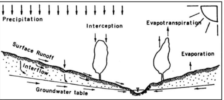
Figure 4: Representation of the hydrological flow process for the PERLND module in HSPF
Climatic Data Center (NCDC) from a station located in Durham, NC (NOAA 2005), with
missing data supplemented by a weather station at Raleigh-Durham International Airport
(RDU) and from the State Climate Office of North Carolina (see Appendix C for details).
2.3 HSPF Model Development
HSPF is fundamentally organized around the development of three modules: (i)
pervious land segments (PERLND) that are subject to infiltration or overland runoff; (ii)
impervious land segments (IMPLND) that are subject solely to overland runoff, and; (iii)
free-flowing reaches or mixed reservoirs (RCHRES) that represent the stream segments
(Bicknell 2001). These modules are primarily focused on the accumulation and transport
of: (i) water; (ii) sediments, and; (iii) general quality constituents, such as fecal coliform,
nitrogen, phosphorous, etc.
2.3.1 Pervious Land (PERLND) Theory Development
The flow of water (PWAT) in the PERLND module is built around several key
processes (Figure 4), which all
interact as part of the HSPF water
balance. These processes are the
primary driver of quality
constituent movement. Overland
runoff is described by:
67 . 1 3
6
.
0
1
*
*
60
)
(
54
.
2
=
+
SURSE
SURSM
SRC
DELT
SURO
, for SURSM < SURSE
or
(
1.6*2.54( ))
1.67* * 60 ) ( 54 .
2 SURO =DELT SRC SURSM
, for SURSM > SURSE
[1]
where:
SURO
: surface outflow (cm/time step);
DELT60
: total time (hr/time step);
SRC
: routing variable, based upon overland flow plane length and
slope;
SURSM
: mean surface detention storage over time step (cm);
SURSE
: equilibrium surface detention storage over time step (cm).
The amount of water available for overland outflow is influenced by the fraction diverted
to other processes, such as surface storage, interflow, and groundwater flow (developed
more fully in Appendix D). Total overflow is primarily controlled through the
adjustment of overland flow storage, as well as parameters associated with soil
infiltration capacity.
The amount, as well as intensity, of rainfall and runoff that occurs is a critical
component in determining the amount of sediment that is transported over the land
surface. Sediment is mobilized through both washoff and scour, the sum of which
represents the total sediment contribution to receiving waters during each time step.
These two processes are described by:
and
(
)
(
)
(
)
JGER DELT SURO SURS KGER DELT SURO SURS SURO SCRSD + + = 60 54 . 2 * * 60 * ) ( 1054 . 247(
)
(
SURS
SURO
)
SURO
DETS
WSSD
+
=
*
[3]
where:
WSSD
: washoff of detached sediment (tons/sq km/time step);
DETS
: detached sediment storage (tons/sq km);
SURO
: surface overflow of water (cm/time step);
SURS
:
surface
storage
(cm);
SCRSD
: scour of soil matrix (tons/sq km/time step);
KGER
: coefficient for scour of the soil matrix;
JGER
: exponent for scour of the soil matrix.
Total load estimates are most sensitive to the adjustment of the amount of detached
storage that is available in each land segment.
Because fecal coliforms in runoff have been observed to exist in a
sediment-associated, as well as a “free” (i.e. unattached), form (Characklis et al. 2005; Krometis et
al. 2007), both water and sediment movement heavily influence the transport of fecal
coliform in the quality constituent module (PQUAL). In PQUAL, overland mobilization
and transport of fecal coliforms is considered as the sum of washed off and scoured
sediment-associated FC, plus the contribution from direct overland flow of free-phase
organisms. These processes are integral to determining the total general quality
constituent load and are described by:
POTFW WSSD
WASHQS = *
,
POTFS SCRSD
SCRQS = *
, and
(
)
(
SURO
WSFAC
)
SQO
SOQO
=
*
1
exp
*
[5]
[6]
where:
WASHQS
: general quality constituent flux associated with sediment washoff
(quantity/sq km/time step);
WSSD
: washoff of detached sediment (tons/sq km/time step);
POTFW
: washoff potency factor (quantity/ton);
SCRQS
: general quality constituent flux associated with soil matrix
scouring (quantity/sq km/time step);
SCRSD
: scour of soil matrix (tons/sq km/time step);
POTFS
: scour potency factor (quantity/ton);
SOQO
: general quality constituent flux associated with washoff from
land surface (quantity/sq km/time step);
SQO
: storage of available quality constituent (quantity/sq km);
SURO
: surface outflow of water (cm/time step);
WSFAC
: susceptibility of quality constituent to washoff (1/cm).
2.3.2 Impervious Land (IMPLND) Theory Development
Similar to pervious surfaces, impervious overland flow is a function of surface
storage and routing. For the accumulation and removal of water flowing over impervious
surfaces, however, the water balance consists of only three subroutines: impervious
retention, overland flow routing, and evaporation (see Appendix E for more detail).
+ =
SURS SURO
SURO SLDS
SOSLD *
where:
SOSLD
: washoff of solids (tons/sq km/time step);
SLDS
:
solids
storage
(tons/sq
km);
SURO
: surface outflow of water (cm/time step);
SURS
: surface storage of water (cm).
While the primary transport mechanism is through surface runoff, daily dry weather
removal by wind is also considered through the loss of a fraction of the total storage.
General quality constituents are modeled in much the same way as for the
PERLND segments, as total washoff will account for direct washoff of both free-phase
and sediment-associated constituents, such that:
(
)
(
SURO
WSFAC
)
SQO
SOQO
=
*
1
exp
*
where:
SOQO
: washoff of quality constituent (quantity/sq km/time step);
SQO
: surface storage of quality constituent (quantity/sq km);
SURO
: surface outflow of water (cm/time step);
WSFAC
: susceptibility of quality constituent to washoff (1/cm).
[8]
2.3.3 HSPF Parameter Development
The EPA has issued suggested soil and water accumulation and removal default
parameters for both the PERLND and IMPLND modules, as well as suggestions for
parameter adjustment given local conditions (USEPA 2000b; USEPA 2006a).
As quality constituent parameters are entirely watershed-specific, the Bacterial
Indicator Tool (USEPA 2000a), an external program, was used to determine land cover-
and subwatershed-specific monthly quality constituent accumulation rates and total
storage limits (see Appendix F). This tool requires user input of land cover areas by
subwatershed, as well as livestock and wildlife population densities and a breakdown of
urban land into commercial, residential, and transportation usages. Though this tool only
explicitly calculates bacterial inputs for urban, forest, cropland, and pasture land covers,
the recommended wildlife population densities and animal fecal coliform production
rates were used to create corresponding outputs for the rangeland, barren, and wetland
land covers.
A full summary of all input PERLND and IMPLND parameters for the hydrology,
solids, and quality constituent modules can be found in Appendix G, with a complete
model code found in Appendix H.
2.4 Parameter Calibration
2.4.1 Data Inventory
For adjustments made regarding the accumulation and removal of water, flow
data from the USGS stream gage (gage ID 0209741955 on Northeast Creek at SR1100
near Genlee (USGS 2007)) were used to compare with modeled flow. Per HSPF
requirements, daily mean stream flow values were obtained for the period of January 1,
2001- September 30, 2006 (the most recent data available), with every day having a
recorded value. Weekly grab sample FC concentrations (Appendix I) were recorded at
three locations (one upstream and two downstream) between the years of 2001-2002 by
the Triangle Wastewater Treatment Plant (WWTP)
6as part of their NPDES monitoring
program, with supplemental data for this period available from USEPA STORET
(USEPA 2006b). However, there were several incidences of “soft” data, for example,
measurements that were only indicated as being greater than a certain threshold. In those
instances, these soft data points were removed from the dataset before analysis. Because
sufficient data points were only available for this two year window, calibration of FC
parameters was completed for data corresponding to January 1, 2001 – December 31,
2001 for both a downstream (Reach 5) and an upstream reach (Reach 3), with validation
completed at both sites for the period January 1, 2002 – December 31, 2002.
2.4.2. Hydrology Calibration
Modeled in-stream flow was compared with observed conditions by using an
external hydrology calibration program, HSPEXP (Lumb et al. 1994). Based upon
literature examining the sensitivity of hydrological parameters in HSPF (Al-Abed and
Whiteley 2002), PERLND parameters related to upper and lower zone nominal storage
Figure 5: Modeled flow at Reach 11 vs. observed USGS gauge flow data.
and infiltration capacity were refined, as were the initial storages for both the PERLND
and IMPLND processes. Since the greatest concern for microbial concentrations is
generally during the summer months and periods of high flow following storm events,
calibration, though performed continuously for the entire period of available data,
focused upon ensuring that summer storm event modeled volumes were as close as
possible to observed volumes over those same storm events. Ultimately, a difference of
less than 5% was present between total modeled and observed summer storm event
volumes over the period January 1, 2001- December 31, 2005 (Figure 5 shows a
representative subset of this period), as well as a total volume difference of less than 15%
throughout the entire model simulation period
7.
0 20 40 60 80 100 120 140 160 180 200
Jan-04 Feb-04 Mar-04 Apr-04 May-04 Jun-04
F
lo
w
(c
fs
)
Modeled Observed
2.4.3 Fecal Coliform Calibration
In terms of adjusting parameters affecting in-stream FC concentrations, previous
studies suggested that the greatest sensitivity was found in PERLND parameters (Paul et
al. 2004). However, because of the increasing urbanization that is occurring in Northeast
Creek watershed, IMPLND parameters routinely yielded greater effects upon in-stream
FC concentrations. Therefore IMPLND parameters associated with overland storage, as
well as the minimum overland flow to remove 90% of built-up FC organisms and the
maximum FC storage potential, were adjusted to calibrate modeled in-stream FC
concentrations for Reaches 3 and 5 with observed FC data from January 1, 2001 -
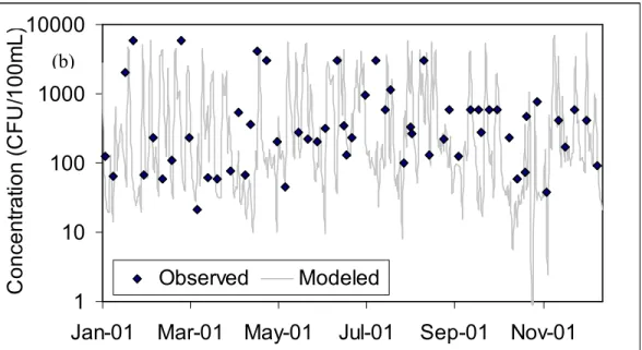
December 31, 2001 (Figure 6a-b).
1 10 100 1000 10000
Jan-01 Mar-01 May-01 Jul-01 Sep-01 Nov-01
C
on
ce
nt
ra
tio
n
(c
fu
/1
00
m
L)
Modeled Observed
Figure 6: Comparison of Modeled vs. Observed in-stream FC concentrations for (a) Reach 3 and (b) Reach 5 during calibration.
1
10
100
1000
10000
Jan-01 Mar-01 May-01
Jul-01
Sep-01 Nov-01
C
o
n
ce
n
tr
a
tio
n
(C
F
U
/1
0
0
m
L
)
Observed
Modeled
For a policy context that is primarily concerned with the identification and
adjustment of bacterial concentrations, it is acceptable to make recommendations based
upon order of magnitude estimations (Dorner et al. 2006). Therefore, quantification of
error between observed and modeled data took the form of determining the percentage of
modeled data points that fell within one order of magnitude of the observed value
8. For
Reach 5, 88% of modeled values (51 out of 58) fell within one order of magnitude of
observed data, and, for Reach 3, 84% of values (42 out of 50) met this criterion
(Appendix J). Further examination revealed a nonparametric Spearman’s rank
correlation coefficient of 0.49 for Reach 5 and 0.52 for Reach 3, with a significance of
greater than 0.001 for observed and modeled dataset.
8Because HSPF outputs on a daily time step, and observed grab samples can be taken at any point in that day, error estimation was completed based upon a three-day best estimate that would allow points to be more accurately compared (Russo 2007).
2.5 BMP Analysis Framework
Though the science of bacterial source characterization and quantification has
been the subject of increasing study (Whitlock et al. 2002; Burnes 2003; Jamieson 2004;
Weiss et al. 2006), as yet there has been no broad agreement on a standardized method to
identify a source control strategy that will most efficiently meet regulatory requirements.
To that end, a linear programming framework is suggested such that an objective function,
which is equal to the total costs associated with a BMP implementation plan, is
minimized while ensuring that in-stream FC concentrations are reduced to compliant
levels. This cost minimization will take the following form:
)
(
)
,
(
)
,
(
jk ijk i jk ijk i ii
X
F
M
X
F
O
A
C
Z
=
+
+
subject to:
=
Y
iX
jkF
ijkQ
kR
complianceR
*
(
*
)
*
where:
C
i: Capital cost of construction of BMP i
($);
M
i: Present value cost for 20-year maintenance of BMP i ($);
O
i: Opportunity cost
9associated with area of BMP i ($/acre);
X
jk: Area of land cover k
in subwatershed j
(acre);
F
ijk: Fraction of land cover k
in subwatershed j
contributing to BMP i;
A
ij: Surface area required for BMP i
in subwatershed j
(acre);
9In this analysis, opportunity costs only account for the cost of land that would be surrendered for a structural BMP, meaning that any loss of economic benefits that could have been gained through that land parcel were not included.
[10]
R
: Watershed reduction in FC loading, in colony forming units (CFU);
Y
i: Efficiency of BMP i
(FC fraction removal);
Q
jk: Yearly FC loading for land cover k
in subwatershed j
(CFU/acre).
For this set-up, X
jk(Appendix B), Q
jk(Appendix M), Y
i(Table 1, synthesis of
Appendix K), and C
i, M
iand O
i(Wossink and Hunt 2003; USEPA 2005) are all known.
R
complianceis calculated from HSPF as a measure of the difference between in-stream FC
quantities at baseline and regulatory-compliant conditions. F
ijkis the only unknown
parameter in this model and is allowed to vary such that runoff from one particular land
segment is not intercepted by multiple treatment controls in what is known as a
“treatment train.” Though it is technically feasible that such a system could be used, the
effects of such systems on removal efficiencies are not clearly understood and are
therefore not considered in this analysis, but could be necessary should the present
suggested model prove unable to ensure sufficient reductions (VADCR 2004).
required to meet the necessary reductions. However, it is the responsibility of the
watershed planner to ensure that these individual BMPs will be located in a spatially
optimal manner (Zhen et al. 2004; Perez-Pedini et al. 2005).
Though not incorporated into this linear programming framework, non-structural
BMPs were also considered in this analysis, and, at least for this representative watershed,
were necessary for ensuring regulatory compliance without requiring extraordinary costs.
The incorporation of non-structural BMPs has the effect of reducing pollutant loading to
the structural BMPs, thereby increasing their efficiency and extending their service life.
Research has shown that educational initiatives, including television and radio spots,
flyers and brochures, and public signage, can have an effect upon human behavior, as
well as garner public support for other control initiatives (Dietz et al. 2004), though
television ads have been shown to have the greatest capacity to reach the public (Schueler
2000). Another non-structural BMP, street sweeping can have a significant impact on FC
loads from impervious urban surfaces (Zariello et al. 2002), reducing the total load along
streets by as much as 50% when performed routinely, particularly when sweeping occurs
during extended dry periods so as to minimize the effects from the first-flush
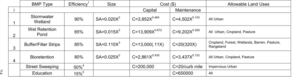
BMP Type Efficiency1 Size Cost ($) Allowable Land Uses
i Capital Maintenance
1
Stormwater
Wetland 90% SA=0.020X2 C=3,852X0.484 C=4,502X0.153 All Urban
2
Wet Retention
Pond 65% SA=0.015X2 C=13,909X0.672 C=9,202X0.269 All Urban, Cropland, Pasture
3 Buffer/Filter Strips 85% SA=0.110X
3 C=13,000(.11X) C=20(320X) Cropland, Forest, Wetlands, Barren, Pasture,
Rangeland
4 Bioretention 80% SA=0.025X
2 C=2,861X0.438 C=3,437X0.152 All Urban, Cropland, Pasture
Street Sweeping 50%4 C=200,000 C=20/curb mile Impervious Urban
Education 15%5 C=650000 All
1 Synthesis of structural BMP efficiency review from Appendix K 2 Wossink and Hunt 2003
3 USEPA 2005 4 Zariello et al. 2002 5 Dietz 2004
Table 1: Summary of BMP characteristics that were used in the optimization analysis (full compilation of sources found in Appendix K).
Chapter III
Results
A strategy for selecting a least-cost mitigation strategy for microbially-impaired
water bodies has been suggested that could be incorporated into the existing TMDL
policy framework. HSPF allows these optimized source control strategies to be verified
by modeling the watershed under suggested conditions. If properly implemented, these
reduction strategies will be an important first step in removing Northeast Creek, or other
water bodies to which this framework is applied, from the list of impaired water bodies,
though great responsibility will lie with those who have been tasked with implementation
and upkeep of a proposed integrated pollution control system.
3.1 Model Validation
Output from the HSPF model was used to verify that results were consistent with
previous work showing that overland FC contributions increase with both rainfall and
temperature (Figure 7). Examinations of overland contributions reveal that the highest
aggregate monthly loads occurring during those months with the largest aggregate
Figure 7: Cumulative monthly rainfall and modeled FC contributions from Subwatershed 1. 0.00E+00 5.00E+08 1.00E+09 1.50E+09 2.00E+09 2.50E+09 3.00E+09
Mar-02 Sep-02 Mar-03 Sep-03 Mar-04 Sep-04
F C L o ad (C F U ) 0 2 4 6 8 10 12 R ai n fa ll (i n .)
FC Load Rainfall
Spring and Summer Spring and Summer Spring and Summer
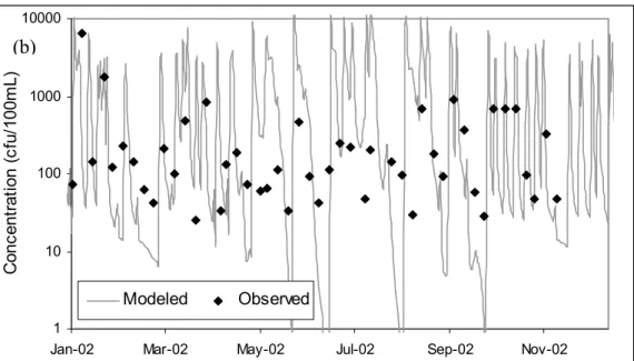
Validation of the calibrated model was completed using in-stream FC
measurements from January 1,2002- December 31, 2002 (Figure 8a-b).
1
10
100
1000
10000
Jan-02
Mar-02
May-02
Jul-02
Sep-02
Nov-02
Figure 8: Comparison of Modeled vs. Observed in-stream FC concentrations for (a) Reach 5 and (b) Reach 3 during validation.
1 10 100 1000 10000
Jan-02 Mar-02 May-02 Jul-02 Sep-02 Nov-02
C
on
ce
nt
ra
tio
n
(c
fu
/1
00
m
L)
Modeled Observed
Again, as order of magnitude estimations are sufficient in modeling exercises,
quantification of error between observed and modeled data took the form of determining
the percentage of modeled data points that fell within one order of magnitude of the
observed value. For Reach 5, 82% of modeled values (36 out of 44) fell within one order
of magnitude of observed data, and, for Reach 3, 90% of values (43 out of 47) met this
criterion (Appendix J). Further examination revealed a Spearman’s rank correlation
coefficient of 0.42 for Reach 5 and 0.63 for Reach 3, which equates to a significance of
slightly less than 0.001 between modeled and observed data for Reach 5 and greater than
0.001 for Reach 3.
3.2 Regulatory Violation Validation
According to North Carolina regulations, FC concentrations in surface
freshwaters shall not exceed a 5-consecutive sample geometric mean concentration of
200 CFU/100mL, nor exceed 400 CFU/100mL in more than 20% of grab samples
Figure 9: Modeled in-stream 5-day running geometric mean concentration at locations above (Reach 3) and below (Reach 5) the Triangle Wastewater Treatment Plant.
(NCDENR 2004). Consistent with its impaired designation, model results confirm that
Northeast Creek regularly violates this standard (Figure 9). For Reach 3, which is
directly upstream of the WTWTP, more than 40% of all in-stream geometric mean
concentrations and 29% of all daily samples violate North Carolina state standards for the
period of January, 2005-June, 2006
10. For the same period, approximately 30% of
geometric mean concentrations and 23% of all daily samples were in violation for
reaches below the WWTP, indicating that WWTP effluent generally dilutes in-stream FC
concentrations (see Table 2 for further explanation).
0 500 1000 1500 2000 2500 3000 3500 4000 4500
Jan-05 Mar-05 Jun-05 Sep-05 Dec-05 Mar-06 Jun-06
G
e
o
m
e
tr
ic
M
e
a
n
(C
F
U
/1
0
0
m
L
) RCH3
RCH5 Standard
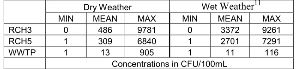
Table 2: Summary of in-stream and effluent FC concentrations for the period of January 1, 2005 - June 30, 2006.
Dry Weather Wet
Weather
11MIN MEAN MAX MIN MEAN MAX
RCH3 0 486 9781 0 3372 9261
RCH5 1 309 6840 1 2701 7291
WWTP 1 13 905 1 11 116 Concentrations in CFU/100mL
As shown, average modeled in-stream FC concentrations under wet weather
conditions are nearly an order of magnitude larger, further confirming the importance of
storm events for FC transport. Reach 3 is prone to higher in-stream FC concentrations
due to the presence of significant amounts of impervious surfaces in the upper reaches of
the watershed. Due to comparitively much lower mean FC concentrations in the WWTP
effluent, mean in-stream FC concentrations below the WWTP will generally be lower
due to dilution.
3.3 Source Loading Identification
Similar to results from previous work (Garcia-Armisen and Servais 2007),
modeled results indicate that impervious surfaces in urbanized watersheds routinely yield
the vast majority of in-stream FC loading when wastewater discharge is regulated by
advanced treatment processes, though this relationship will not hold for watersheds
dominated by agricultural land cover. Point source FC contributions from the WWTP,
however, are still greater than pervious surface contributions (Figure 10, with more detail
in Appendix L).
Figure 10: Relative fractions of sources of in-stream fecal coliform loading.
0% 10% 20% 30% 40% 50% 60% 70% 80% 90% 100%
2002 2003 2004
Pervious Impervious WWTP
Given that there are currently very few nonpoint source controls in place in the
watershed
12, these results indicate that reductions from impervious land segments will be
critical in reducing in-stream concentrations to meet regulatory requirements. This also
suggests that controls will be most effective when placed in subwatersheds having the
greatest amount of impervious surfaces, particularly for those reaches that do not
experience the effects of dilution from WWTP effluent.
3.4 Nonpoint Source Controls
The choice and placement of BMPs is at the heart of an effective watershed
restoration plan. Though many new development projects are required to include BMPs
to counteract the negative effects of land use changes, this does not address the adverse
effects associated with pre-existing development. Therefore, the selection of BMPs in
this analysis will be made under the assumption that any future net increases in FC
loading associated with land use changes will be addressed accordingly (such as is
suggested in Randolph(2004)), allowing this work to be concerned solely with addressing
present conditions.
3.4.1 Source Control Examination
Initially, a mixture of nonpoint source BMPs were introduced into the HSPF
model was altered to see if necessary reductions in in-stream FC concentrations could be
achieved solely through the implementation of either structural or non-structural nonpoint
source controls. Maximum coverage of structural nonpoint source controls took the form
of stormwater wetlands for urban drainage and buffer strips for all other permeable land
cover runoff
13. Non-structural controls took the form of educational initiatives, increased
street sweeping, and wildlife exclusion (to prevent direct deposits from wildlife).
However, model output indicated that sufficient reductions could not be achieved along
the entire impaired stream length through the implementation of either structural or
non-structural nonpoint source controls alone (Figure 11a-b).
Figure 11: Comparison of source reduction control strategies with baseline conditions for locations (a) above and (b) below the WWTP.
0 500 1000 1500 2000 2500 3000 3500 4000 4500
Jan-05 May-05 Sep-05 Jan-06 May-06
C on ce nt ra tio n (C F U /1 00 m L)
Reach 3 Base RCH3 Non-Structural Only RCH3 Structural Only
0 200 400 600 800 1000 1200 1400 1600 1800
Jan-05 May-05 Sep-05 Jan-06 May-06
C o nc en tra tio n (C F U /1 0 0m L)
Reach 5 Base RCH5 Non-Structural Only RCH5 Structural Only
It is important to note that it was feasible to achieve in-stream regulatory
compliance for Reach 3 through the introduction of structural nonpoint source controls
alone, though this was not possible in Reach 5, indicating that the WWTP effluent
(a)
concentrations at this instance were sufficient to violate in-stream standards in the
absence of any other FC loading within the watershed. Therefore, it is imperative for the
WWTP to able to ensure that an additional 1-log removal of the peak effluent loads over
the period of January 1, 2005-June 30, 2006 can occur.
3.4.2 BMP Optimization Results
Before the linear optimization model was run using What’s Best (Lindo 2006),
additional point source controls (representing the assurance of an additional 1-log
removal of peak effluent concentrations) and new non-structural nonpoint source controls
(representing education initiatives and street sweeping
14) were introduced into the model.
Then, it was possible to determine the lowest cost
alternative to address the balance of excess
overland FC loadings through a mix of structural
BMPs. A summary of the least cost strategy is
presented (Table 3, with full details in
Appendix N). This scenario minimizes the costs
that would be garnered from capital, 20-year
maintenance, and land purchase costs.
The suggested control strategies were
then introduced to the calibrated and validated
HSPF model to verify that modeled 5-day
running geometric mean concentrations do not exceed the state-mandated threshold at
any point over the study time period, including the addition of a margin of safety (MOS)
14 Note that, though wildlife exclusion was initially considered as a potential non-structural BMP, this was not included in the final analysis given concerns over whether this could effectively be implemented, as well as the desire to preserve the natural habitats that exist.
All Urban Stormwater
Wetlands
Coverage Total Cost
Sub 1 51.3% $671,245
Sub 2 100% $2,554,782
Sub 3 100% $1,544,464
Sub 4 100% $1,640,847
Sub 5 100% $830,079
Sub 6 19.6% $218,551
Sub 7 100% $163,661
Sub 8 100% $606,605
Sub 9 - -
Sub 10 100% $843,030
Sub 11 0% $0
$18,149,800
Figure 12: Modeled in-stream running 5-day geometric mean FC concentrations following implementation of least cost BMP allocation scenario.
Table 4: Summary of costs associated with management practices for the control of FC in Northeast Creek watershed
(USEPA 2007d) corresponding to 10% of the standard (Figure 12). This MOS works to
ensure that storm events (which are the primary cause of regulatory non-compliance from
nonpoint source pollution) larger than those examined would not adversely affect the
water body to a point in which it would be out of compliance.
0 20 40 60 80 100 120 140 160 180 200
Jan-05 May-05 Sep-05 Jan-06 May-06
C o n ce n tr at io n (C F U /1 00 m L)
RCH3 RCH5 Standard + M.O.S
3.4.3 BMP Costs
As seen, the 20-year costs of structural BMPs
alone would be nearly $18,200,000 in present value
terms (Table 4). 20-year educational initiative costs
of $650,000 are based on the spending budgeted by
the North Carolina Clean Water Education
Partnership for similar purposes (Bruce 2006).
With the inclusion of street sweeper costs of
slightly more than $3,000,000, the total value of
Education $0.65 M
Street Sweeping
Capital $0.68 M
O&M $2.37 M
Structural BMPs
Capital $5.13 M
O&M $5.31 M
Opportunity $7.71 M
structural and non-structural BMPs rises to around $21,850,000.
In order to cover the costs of the proposed management strategy, each resident
(including future residents based upon current population growth trends) would need to
contribute $57/year toward the construction and maintenance of this system of BMPs
(Appendix O). These costs are substantial, and some point of reference regarding the
value that local residents might place on water quality should provide a useful basis for
comparison. Though residents in Northeast Creek watershed have not been directly
surveyed to determine their willingness to pay for water quality improvements, research
in the nearby Catawba River basin of western North Carolina has shown that residents
were willing to pay $139/year for five years toward water quality protection, to ensure
that the Catawba remains acceptable as both a drinking water source and recreational
water body (Eisen-Hecht and Kramer 2002; Kramer and Eisen-Hecht 2002).
Chapter IV
Final Remarks
Due to the large number (both nationally and in North Carolina) of microbially
impaired water bodies, it is crucial that more concentrated efforts are made to address this
issue. This work has done so within the framework of developing a watershed restoration
plan for one such impaired water body, Northeast Creek, which is in a representative area
of the Piedmont region of North Carolina. This process included the development and
calibration of a nonpoint source pollution model focused on fecal coliforms, as well as a
strategy to identify a least-cost mitigation strategy to ensure regulatory compliance.
HSPF model calibration was completed using available physical and biological
data, with validation yielding greater than 80% of modeled values within an acceptable
range of observed data. Ensuring model validation was necessary before utilizing the
BMP optimization model. Results from this analysis reveal that the suggested mitigation
strategy will have a 20-year present value cost of a little over $20,000,000. This
per year toward the cost of this mitigation plan. This strategy has suggested both
structural and non-structural initiatives to ensure regulatory compliance. However, the
potential benefits of these controls are contingent upon the incorporation of nonpoint
source controls when land use changes cause a net increase in overland microbial loads.
The recommendations that have been presented in this report represent the
findings from the usage of the best available technology for watershed modeling that
exists at the moment. As with any modeling application, however, there are
shortcomings that do exist, such as the lack of sufficient data to perform continuous fecal
coliform calibration and validation, the lack of specificity regarding overland fecal
coliform loadings, and uncertainties with regard to sanitary sewer and septic system
failure rates, all of which lead to rather large error bounds on the magnitude of overland
contributions. In addition, there exist large uncertainties on actual versus theoretical fecal
coliform removal capability from the selected best management practices. Given these
conditions, therefore, it is important to interpret model results with caution given that
these results are an accurate representation of the underlying model. Further efforts to
improve this work would revolve around better identification of overland sources and
their magnitudes, as well as more refined estimations of fecal coliform removal from
structural and non-structural best management practices.
Appendix A
Spatial Representation of Northeast Creek Watershed
Appendix B
BASINS subwatershed land use distribution (acres)
Pervious Impervious
Urban Cropland Forest Wetland Barren Pasture Rangeland Urban
Subwatershed 1 556 22 807 87 22 65 65 556
Subwatershed 2 1085 52 2221 258 52 310 103 1085
Subwatershed 3 656 18 108 288 - 54 36 656
Subwatershed 4 697 65 1329 227 32 130 65 697
Subwatershed 5 353 - 423 197 - 28 56 353
Subwatershed 6 475 203 4270 668 203 271 203 475
Subwatershed 7 70 52 1095 313 17 52 70 70
Subwatershed 8 258 172 3836 401 - 458 344 258
Subwatershed 9 - 18 622 178 - 45 27
-Subwatershed 10 358 29 387 172 14 14 100 358
Subwatershed 11 3 3 113 8 - 19 11 3
Percentage of Total Watershed Area
14.8% 2.1% 49.8% 9.2% 1.1% 4.7% 3.5% 14.8%
Table B.1: Allocation of land use by subwatershed.