Polarization-Sensitive Optical Coherence
Tomography to Study Diffusion of Plasmonic Gold
Nanorods – a Novel Tool for Optical Bioimaging
Raghav K. Chhetri
A dissertation submitted to the faculty of the University of North Carolina at Chapel Hill in partial fulfillment of the requirements for the degree of Doctor of Philosophy in the Department of Physics and Astronomy.
Chapel Hill 2013
Approved by:
Amy L. Oldenburg
Christian Iliadis
Michael R. Falvo
Otto Zhou
c
○2013
Abstract
RAGHAV K. CHHETRI: Polarization-Sensitive Optical Coherence Tomography to Study Diffusion of Plasmonic Gold Nanorods – a Novel Tool for Optical Bioimaging
(Under the direction of Amy L. Oldenburg)
Optical Coherence Tomography (OCT) is an imaging tool that performs
micron-resolution, non-invasive, cross-sectional imaging by measuring the echoes of
backscat-tered light. In this thesis, a custom-designed polarization-sensitive OCT (PS-OCT)
system is discussed, which is implemented in using plasmonic gold nanorods (GNRs)
as diffusion probes. PS-OCT imaging is undertaken in Newtonian fluids and validation
of rotational and translational diffusion of GNRs with the Stokes-Einstein relation is
presented via analysis of the autocorrelations of the OCT signals. Diffusion of GNRs in
non-Newtonian fluids is also studied and the frequency-dependent viscoelasticity is also
explored using generalized Stokes-Einstein relation. Furthermore, diffusion of GNRs
in the “correlation length ≥ probe” regime is discussed in low concentration polymer
solutions. Biological samples such as porous extracellular matrix (ECM) and in vitro
mucus are explored using PEGylated GNRs as diffusion probes with PS-OCT imaging.
The diffusion of GNRs was found to be sensitive to changes in the ECM induced either
by ECM-remodeling fibroblasts or by changes in the ECM concentration. In mucus,
the diffusion of GNRs was observed to be slowed down by less than 7-fold compared to
the solvent, suggesting that the GNRs are able to readily navigate between the mucus
mesh and avoid being readily trapped, thereby illustrating the potential GNRs hold
in drug-delivery across the mucus barrier to the epithelial layers in lung airways. The
capability of OCT to map diffusing GNRs and speckle fluctuations resulting from other
mam-mary epithelial cells cultured in 3D with fibroblasts, to study normal and pre-malignant
architectural cues, carried out using the custom-designed OCT system is also presented
in detail. The integration of PS-OCT imaging with the measurement of diffusing GNRs
in biological samples enables OCT to perform functional imaging to supplement its
ex-cellent structural imaging capability. This thesis presents a platform for extending the
reach of OCT imaging to the exciting fields of microrheology and bio-rheology, which
holds tremendous promise in the assessment of micro- and nano- scale viscoelasticity of
Acknowledgements
I feel truly fortunate to have the blessing, good wishes, love, support and
encourage-ment from my family. Without the solid foundation they laid for me, this work won’t be
possible. Thank you so much! My warmest thanks to my better half, Lachhita Neupane,
for always being there to support me, providing apt humor on stressful grad-school days
to lighten me up, and helping me to see the forest for the trees.
I’d like to acknowledge the guidance, supervision, and support of my advisor Dr.
Amy L. Oldenburg throughout my time in the Coherence Imaging Laboratory. I’d like
to thank her for giving me the opportunity to work in her group, which exposed me to
the exciting field of biomedical optics. I’m grateful to all present and former members
of the group, whom I have had the opportunity to interact with and learn from. I would
like to thank Dr. Joseph B. Tracy in the Department of Material Science and
Engineer-ing at North Carolina State University for synthesizEngineer-ing and providEngineer-ing several batches
of gold nanorods, and also for timely advice, guidance, and suggestions to research
queries. It was my pleasure to collaborate with Dr. Tracy’s group and I’d like to thank
his group members, Krystian A. Kozek, Aaron C. Johnston-Peck, and Wei-Chen Wu,
for their contribution in synthesizing and characterizing the gold nanorods. I am also
indebted to the University of North Carolina Cystic Fibrosis and Pulmonary Research
and Treatment Center, particularly David B. Hill and Brian Button for culturing and
providing mucus samples,in vitro hBE cultures, and also engaging in helpful discussions
helpful discussions on polymer physics and mucus rheology. I would also like to thank
Dr. Melissa Troester in the UNC Gillings School of Public Health and her research group
for providing cells for the breast cancer study, their assistance in establishing protocols
for cell cultures in 2D and 3D, and numerous insightful discussions on our collaborative
research on breast cancer pre-malignancy.
I would also like to thank Timothy O’Brien in the Computer Integrated Systems for
Microscopy and Manipulation (CISMM) at UNC, Chapel Hill for allowing me to use his
lab space for cell cultures, his insights to biology-related queries, and his willingness to
help at all times. Thanks are also due to Amanda C. Sullivan, Zachary F. Phillips, and
Jason M. Cooper for their contributions in several research projects, and I am grateful
for the opportunity to work with & mentor such outstanding undergraduate students. I
am also indebted to the faculty members who helped me understand the fundamentals
of physics during my time as a graduate student. I feel fortunate to have had excellent
faculty members to learn from, which include Yue Wu, Charles R. Evans, Jonahan
Engel, Laura Mersini-Houghton, Jainping Lu, Otto Zhou, Dmitri Khveshchenko, the
late Eugen Merzbacher, Michael Rubinstein, Caterina Gallippi, and Daniel J. Gauthier
(Fitzpatrick Institute for photonics) during my time at UNC, Chapel Hill. I’d also like
to acknowledge my Masters and PhD committee members, Rene Lopez, Otto Zhou, Yue
Wu, Michael R. Falvo, Christian Iliadis, and Amy L. Oldenburg, for their role in helping
me set my research goals and guidance in achieving them.
My gratitude also goes to the 2010 Nano-biophotonics Summer School at the
Uni-versity of Illinois, Urbana-Champaign for piquing my interest in the field of biomedical
optics. In particular, I am indebted to Gabriel Popescu, Stephen Boppart, and Samir
Sayegh for their continued encouragement and suggestions beyond the confines of the
summer school. I would also like to thank the Center for Biomedical OCT Research
opportunity to learn the principles, functionality, and clinical relevance of various OCT
systems.
Lastly, I’d like to acknowledge my fellow Tarheels in the Department of Physics and
Astronomy at UNC Chapel Hill and the good friends I have made outside the department
for their support and encouragement at various junctures in my graduate-student-life.
I am also indebted to my officemates, Brian Pohl and Michael Good in particular, for
engaging in discussions on important scientific problems in their fields and beyond, and
Table of Contents
Abstract . . . iii
List of Tables . . . xiii
List of Figures . . . xiv
List of Abbreviations . . . xvii
1 Introduction . . . 1
1.1 Motivation . . . 1
1.2 Thesis contributions . . . 2
1.3 Thesis outline . . . 3
2 Light scattering and Brownian motion . . . 5
2.1 Light scattering . . . 5
2.2 Dynamic light scattering . . . 8
2.2.1 Heterodyne detection scheme . . . 13
2.3 Brownian motion and diffusion . . . 15
2.3.2 Optically isotropic scatterers . . . 21
2.3.3 Optically anisotropic scatterers . . . 22
2.4 Motivation for Optical Coherence Tomography . . . 25
3 Optical Coherence Tomography system development . . . 28
3.1 Optical Coherence Tomography . . . 28
3.1.1 Time domain OCT . . . 31
3.1.2 Spectral domain OCT . . . 37
3.2 Design of spectral domain PS-OCT system . . . 41
3.3 Data acquisition and image processing . . . 47
4 Gold Nanorods . . . 52
4.1 Introduction . . . 52
4.2 Cross-polarized and isotropic autocorrelations . . . 54
4.3 GNRs for OCT based diffusion imaging . . . 56
4.4 Experimental Method . . . 58
5 Diffusion of GNRs using OCT . . . 64
5.1 Rotational diffusion in Newtonian fluids . . . 64
5.1.1 Introduction . . . 64
5.1.2 Method and results . . . 66
5.1.3 Conclusion . . . 74
5.2.1 Calibration: CTAB-coated GNRs . . . 75
5.2.2 Calibration: PEGylated GNRs . . . 79
5.3 Non-Newtonian fluid: polymer solutions . . . 83
5.3.1 Diffusion of GNRs in semi-dilute PEO solutions . . . 87
5.3.2 Diffusion in “correlation length ≥ probe” regime . . . 96
6 Biological studies . . . 100
6.1 GNRs in 3D tissue culture models . . . 100
6.1.1 Delivery and diffusion of GNRs . . . 101
6.1.2 GNRs diffusion as a function of collagen I concentration . . . 104
6.1.3 GNRs diffusion in fibroblast cultures . . . 107
6.1.4 GNRs in mammary epithelial cell culture . . . 109
6.2 GNRs in in vitro hBE mucus . . . 112
6.2.1 GNRs diffusion vs mucus concentration . . . 114
6.2.2 GNRs in in vitro mucus over ALI culture . . . 117
6.3 OCT Imaging: 3D epithelial-fibroblast cultures . . . 121
6.3.1 Introduction . . . 122
6.3.2 Method . . . 124
6.3.3 Results . . . 128
6.3.4 Discussion . . . 132
6.3.5 Supplementary . . . 135
7 Conclusion . . . 141
7.1 Utility and potential impact . . . 143
A MATLAB codes . . . 145
A.1 Diffusion coefficients from OCT signals . . . 145
List of Tables
3.1 Parameters of the custom-built PS-OCT system. . . 46
5.1 CTAB-coated GNRs: τ1/e of g
(1)
HV(τ) and g (1)
ISO(τ), and the diffusion
coef-ficients . . . 75
5.2 PEGylated GNRs: τ1/eofg (1)
HV(τ) andg (1)
ISO(τ), and the diffusion coefficients 80
5.3 Estimation ofRg, c∗, and polymer number density in PEOs of molecular
weightMw. . . 88
5.4 PEGylated GNRs: τ1/e of g
(1)
HV(τ) and g (1)
ISO(τ), and the diffusion
coeffi-cients in different concentrations of PEO1M . . . 90
5.5 PEGylated GNRs: τ1/e of g
(1)
HV(τ) and g (1)
ISO(τ), and the diffusion
coeffi-cients in PEOs of different molecular weight (c = 2.5% w/w). . . 93
5.6 PEGylated GNRs: τ1/e of g (1)
ISO(τ),DT and relative viscosities in PEO4M
in the “correlation length ≥probe” regime. . . 97
List of Figures
2.1 A basic light scattering setup . . . 7
2.2 Pictorial representation of an autocorrelation function . . . 12
2.3 Components of polarizability tensors in a rod . . . 24
2.4 Source spectrum and interference fringes . . . 26
3.1 Optical coherence tomography (OCT) imaging . . . 29
3.2 TD-OCT system . . . 33
3.3 SD-OCT system . . . 38
3.4 Custom PS-OCT system . . . 42
3.5 Single-camera spectrometer . . . 45
3.6 PS-OCT images of a lambertian scatterer . . . 49
3.7 PS-OCT images of Collagen I (2 mg/ml) . . . 50
3.8 Retardance image of smooth chicken muscle . . . 50
4.1 Tunability of GNRs LSPR mode . . . 53
4.2 Absorbance spectrum, size analysis of GNRs . . . 57
4.3 Representative B-mode and M-mode PS-OCT images with GNRs . . . . 61
5.1 PS-OCT interferometer and representative M-mode images . . . 67
5.2 Cross-polarized autocorrelation, gHV(1), for several viscosities . . . 69
5.3 Comparison of experimentalDR with a theoretical model . . . 71
5.5 Rotational and translational diffusion calibration of CTAB-coated GNRs 77
5.6 Sample inverse-exponential fittings to the experimental autocorrelations . 79
5.7 Rotational and translational diffusion calibration of PEGylated GNRs . . 81
5.8 DR/DT of GNRs . . . 82
5.9 Concentration regimes in polymer solutions . . . 84
5.10 G0 and G00 for 60 nm microspheres diffused in water . . . 86
5.11 G0 and G00 for GNRs diffused in a Newtonian fluid . . . 87
5.12 MSD of PEGylated GNRs (size: 62 ± 10 nm by 18 ± 4 nm) vs concen-tration in PEO1M . . . 91
5.13 G0 and G00 for 1.25%, 2.50%, and 5% PEO1M samples . . . 91
5.14 MSD of PEGylated GNRs in 2.5% PEO1M, 2.5% PEO4M and 2.5% PEO8M samples . . . 94
5.15 G0andG00for PEOs of different molecular weights (constant concentration of 2.5% w/w). . . 95
5.16 gISO(1) (τ) in PEO4M in the “correlation length ≥probe” regime. . . 97
6.1 B-mode PS-OCT images of collagen I:Matrigel ECM before and after the addition of PEGylated GNRs. . . 102
6.2 gHH(1) (τ) and gHV(1) (τ) in collagen I:Matrigel ECM. . . 103
6.3 gISO(1) (τ) in the solvent and collagen I:Matrigel ECMs. . . 105
6.4 B-mode PS-OCT images of collagen I with and without GNRs. . . 106
6.5 gISO(1) (τ) and DT in collagen I at different concentrations. . . 107
6.6 B-mode PS-OCT images of tissue cultures with RMFs. . . 108
6.8 PS-OCT B-mode images of MCF10A cells cultured in collagen I:Matrigel
ECM in presence of GNRs. . . 110
6.9 PS-OCT M-mode images of MCF10A cells cultured in collagen I:Matrigel ECM in presence of GNRs. . . 111
6.10 B-mode OCT images, histology of CF and normal lung airways. . . 113
6.11 gISO(1) (τ) andDT in purifiedin vitro mucus obtained from hBE ALI inter-face cultures. . . 115
6.12 gISO(1) (τ) and DT in unperturbed in vitro mucus obtained directly from hBE ALI interface cultures. . . 116
6.13 B-mode PS-OCT images of 2.5% in vitro mucus and hBE ALI culture with mucus. . . 117
6.14 B-mode PS-OCT images of mucus and hBE ALI culture with mucus in presence of GNRs. . . 119
6.15 PS-OCT M-mode images of mucus with GNRs over an ALI culture. . . . 120
6.16 3D-OCT image acquisition of the co-cultures, and analysis of the shape and size of acini. . . 129
6.17 Acini and lumen size. . . 130
6.18 Asphericity of acini. . . 131
6.19 Schematic diagram of the OCT system . . . 135
6.20 Representative OCT x−z images of 3D cultures at week 2. . . 137
6.21 Representative OCT x−z images of 3D cultures at week 4. . . 138
6.22 Acini size analysis. . . 139
List of Abbreviations
CF Cystic Fibrosis
COPD Chronic Obstructive Pulmonary Disease
CTAB Cetyltrimethylammonium Bromide
DCIS Ductal Carcinoma in situ
DLS Dynamic Light Scattering
DWS Diffusing Wave Spectrsocopy
ECM Extracullular Matrix
FD-OCT Fourier Domain Optical Coherence Tomography
FWHM Full Width at Half Maximum
GNRs Gold Nanorods
GSER Generalized Stokes-Einstein Relation
hBE Human Tracheo-bronchial-epithelial
LCI Low Coherence Interferometry
LSPR Longitudinal Surface Plasmon Resonance
MEC Mammary Epithelial Cells
MNPs Magnetic Nanoparticles
MSD Mean Squared Displacement
NA Numerical Aperture
OCT Optical Coherence Tomography
OPD Optical Path Length Difference
PEG Poly-ethylene Glycol
PEO Poly-ethylene Oxide
PSF Point Spread Function
PS-OCT Polarization Sensitive Optical Coherence Tomography
QWP Quarter Wave Plate
RMF Reduction Mammoplasty Fibroblasts
SD-OCT Spectral Domain Optical Coherence Tomography
SLS Static Light Scattering
SNR Signal to Noise Ratio
SPR Surface Plasmon Resonance
SS-OCT Swept Source Optical Coherence Tomography
Chapter 1
Introduction
1.1
Motivation
Light scattering is a fascinating phenomenon, the consequences of which are both
perplexing and insightful, and has caught the imagination of scientists across the entire
discipline of science. Recent developments in optical bioimaging are unraveling the
ease and flexibility light scattering affords in studying complex biological systems
non-invasively and yet with ultrahigh resolution. Optical Coherence Tomography (OCT) is
an example of such a recently established optical bioimaging tool. OCT implements a low
coherence, infra-red light source with an interferometer, which enables depth-sectioning
of samples by only allowing coherent backscattering of light from various depths in the
sample to interfere with the unaltered light beam backscattered from a reference mirror.
OCT has been established as a powerful research and diagnostic tool in various fields
such as cardiology, pulmonology, urology, oncology, and most notably, opthalmology.
With the advent of faster acquisition tools and rapid improvements in laser sources,
the imaging capability of OCT will inevitably approach and possibly exceed traditional
optical imaging modalities.
capa-bility of OCT makes it even more appealing in biomedical studies. The integration of
functional imaging is explored in this thesis via the design of a custom
polarization-sensitive OCT (PS-OCT) system, which exploits the polarization dependent optical
scattering property of plasmonic gold nanorods (GNRs), and enables the study of their
diffusion in biological fluids such as mucus, and soft gels such as collagen I & Matrigel.
The ability to not only image structural cues but also non-invasively probe the
vis-coelastic properties of such biological fluids and soft solids via the diffusion of nanosized
probes, such as GNRs, presents an immense opportunity in understanding the
micro-and nano- scale rheology of bioiogical samples. Moreover, the knowledge of micro- micro-and
nano- scale diffusion of cylindrical probes such as GNRs sheds light on the diffusion
of various nanoscopic objects (such as viruses, pathogens, toxins etc.) encountered in
biological studies. This thesis aims to supplement the excellent and real-time
visualiza-tion of biological features afforded by OCT with an extension of its applicavisualiza-tions to the
growing fields of microrheology and bio-rheology.
1.2
Thesis contributions
In this thesis, I discuss the polarization dependent and high albedo of plasmon
resonant GNRs combined with the imaging modality of OCT to investigate micro- and
nano- scale diffusion. Development of a custom polarization-sensitive OCT (PS-OCT)
system is discussed in this thesis followed by a method to probe the rotational and
translational diffusion of GNRs. This work establishes the capability of OCT to image
in two orthogonal polarization channels, and extends its functionality beyond structural
imaging by allowing measurement of the diffusion of GNRs.
Unlike conventional micron-sized and spherical-shaped diffusion probes used in
Dy-namic Light Scattering (DLS), we use GNRs, which offer three main advantages – 1.
fluid, which the micron-sized probes are unable to sense. 2. GNRs depict plasmon
resonance due to the oscillation of their conduction band electrons which increases the
radiative properties of the GNRs. This makes GNRs an excellent choice as efficient light
scatterers. 3. GNRs are optically anisotropic i.e., they scatter light in a
polarization-dependent manner. This enables us to probe their rotational diffusion in addition to
translational diffusion using light scattering.
Additionally, we employ OCT to probe the diffusion of GNRs, which offers two major
advantages over traditional DLS techniques – 1. OCT allows diffusion to be
depth-resolved within a heterogeneous sample. 2. OCT efficiently rejects multiple scattering
from turbid samples and thus enables investigation of probe diffusion in highly scattering
samples.
1.3
Thesis outline
Chapter 2 begins by discussing the fundamentals of dynamic light scattering and
how the Brownian motion of structurally isotropic as well as anisotropic probes can be
characterized from the scattered light. The motivation for using low coherence
interfer-ometry (LCI) to study Brownian motion is presented in this chapter, making way for
the discussion of optical coherence tomography (OCT), an LCI-based technique, in the
next chapter.
Chapter 3 first gives an overview of the principle of OCT through the discussion
of time-domain OCT (TD-OCT) technique. The working principle of spectral domain
OCT (SD-OCT) is then briefly reviewed, and various parameters associated with the
performance of OCT systems are also discussed. The design and development of a
custom PS-OCT system is described next. Characterization of the PS-OCT system,
image acquisition and processing are also presented in this chapter.
use with OCT. The experimental methods including GNRs number density estimation,
data acquisition, and data analysis to relate OCT signals to diffusion coefficients are
presented in this chapter.
Chapter 5 delves into the experimental method of studying Brownian motion using
OCT. It starts out by validating rotational diffusion of GNRs in Newtownian fluids
with the Stokes-Einstein relation. Depth-resolving rotational diffusion to infer viscosity
within a single sample using the established method is also discussed. Next, the method
is extended to translational diffusion of GNRs, and a simultaneous measurement of
rotational and translational diffusion of GNRs over a range of viscosities is discussed.
This chapter further explores the diffusion of GNRs in non-Newtonian fluids such as
polymer solutions, and explores the nanoscale viscoelasticity probed by the GNRs.
Chapter 6 is dedicated to the biological study of the diffusion of GNRs in biologically
relevant tissue-mimicking matrices (collagen I, Matrigel) and fluids (mucus), and
cul-minates with an in-depth imaging study of mammary epithelial-fibroblast 3D cultures
carried out using the custom-built OCT system.
Lastly, chapter 7 summarizes the utility of the imaging modality of OCT and the
proposed method of probing nano- and micro- scale diffusion using GNRs with OCT.
It also explores the potential impacts of this thesis in the fields of bio-rheology and
Chapter 2
Light scattering and Brownian
motion
2.1
Light scattering
Naturally occurring colors such as the bright blue sky, a majestic view of the horizon
during sunrise and sunset, and arching rainbows after a misty rain shower, have long
captured the imagination of humankind. Mankind’s quest to understand such natural
phenomena has today grown into the enormous field of light scattering, and has led to
profound applications in various scientific disciplines.
Light is electromagnetic radiation spanning the frequency range from infrared
(fre-quency of ∼1013 Hz) to ultra-violet (frequency of ∼1017 Hz). Visible light is the range
of electromagnetic spectrum over which our human eyes are sensitive (wavelength range
of ∼400 nm to ∼750 nm). Light can be characterized by its frequency (related to the
wavelength via the speed of light), state of polarization and the direction of propagation.
The phenomenon of light scattering is a result of heterogeneity in the medium, whether
on the molecular scale or on the scale of larger molecular aggregates that result in a
spatial distribution of the refractive index. The basic process underlying scattering is
the absorption of the incident electromagnetic radiation by the molecules in the obstacle
con-sequence of the oscillating electric charges, electromagnetic radiation is emitted (since
accelerating electric charges radiate energy), which we call radiation scattered by the
obstacle. The intrinsic properties of the scattered radiation can be different than that
of the incident radiation. For the purpose of this thesis, we will limit ourselves toelastic
scattering in which the frequency of the scattered radiation is the same as that of the
incident radiation.
The strength of scattering is dependent primarily on polarizability of the scatterers,
the number of scatterers, and the size of the scatterers. When the scatterers are
non-interacting and are sufficiently small compared to the wavelength of light (λo), they can
be considered point-dipole oscillators of the incident radiation (Figure 2.1). This was
first described by Lord Rayleigh in the late 1800s and today bears his name: Rayleigh
scattering. In the regime of Rayleigh scattering, the scattered intensity is observed to be
inversely proportional toλ4o, and the scattering is observed to have insignificant angular
dependence. However, as the particle size approaches or exceeds the wavelength of light,
it can no longer be treated as a single dipole oscillator. The simplest approach then
would be to treat a single particle as an assembly of many dipole scatterers each of which
gives rise to Rayleigh scattering. Although the size of the scatterers plays a critical role
in the treatise of light scattering, the scatterers’ shapes dictate the overall scattering as
well and so does the polarization state of the incident beam. This fact is exploited in
chapter 4 where scattering from GNRs is discussed.
The study of scattering media isn’t limited to the methods of light scattering, as
there are numerous other scattering methods which have their own merits. For
in-stance, X-ray and neutron scattering, due to their small wavelength, are able to probe
smaller structures (on the order of a few angstroms). In comparison, due to significantly
longer wavelengths compared to X-ray and neutron scattering, light is suitable for
Figure 2.1: Point-like scatterers in the scattering volume are irradiated by a plane wave (incident wave vector,ki), and the scattered beam is collected at an angleθs (scattering
wave vector,ks).
years has brought about various light scattering-based advancements in the
characteri-zation of macromolecules, polymers and colloids. Unlike X-ray and neutron scattering,
light scattering techniques are non-invasive & non-ionizing, which is a critical advantage
especially considering biomedical applications. Also, the availability of laser sources,
which provide collimated (spatially coherent) and temporally coherent light, presents
an additional advantage over other scattering methods.
A typical light scattering experiment consists of three basic units: a light source,
a scattering medium, and a detector. In our discussion of light scattering, we are
restricting ourselves to a scattering medium consisting of a dilute ensemble of particles,
so the total scattering signal is the composite of the scattering from all particles within
the illumination volume of the light source. Techniques based on light scattering rely
on analyzing this composite scattered field to retrace the nature or the behavior of
particles that are responsible for the scattering of light. A wealth of information about
diffusion coefficients, and relaxation times of statistical fluctuations, can be extracted
from suitable analysis of the scattered light. Light scattering techniques can be broadly
categorized into two subgroups: static (classic) light scattering (SLS) and, dynamic
(quasi-static) light scattering. In static light scattering, the time-averaged intensity of
scattered light is measured as a function of the scattering angle, and parameters such
as weight-averaged molar mass and radius of gyration of aggregates can be extracted
by following a Rayleigh-Debye-Zimm formalism [1, 2]. In dynamic light scattering, the
quantity of interest is the temporal intensity fluctuation scattered light, and the typical
parameters that can be derived are the hydrodynamic size, and the diffusion coefficients
of the particles. Dynamic light scattering is discussed in more detail in the following
section.
2.2
Dynamic light scattering
Dynamic light scattering (DLS) deals with the analysis of intensity fluctuations of
scattered light which can then be related to the underlying dynamics of the
scatter-ing medium. DLS is the technique behind various commercial light scatterscatter-ing based
particle-sizers. A monochromatic laser source irradiates a dilute solution containing the
particles to be characterized. The scattered field fluctuates due to the stochastic
mo-tion of the scatterers and this signal is collected by various detecmo-tion schemes. With a
priori knowledge of the solvent, the analysis of this temporal signal is used to infer the
hydrodynamic size and size distribution of the particles. Alternatively, using probes of
known size, shape, and low polydispersity, the physical property of the solvent such as
viscosity in case of Newtonian fluids and viscoelasticity in case of non-Newtonian fluids
can be elucidated from the measured diffusion coefficients of the probes.
To understand the analysis involved in DLS experiments, let’s start by considering a
in the sample. In complex notation, the incident field is represented as:
~
Ei(~r, t) =Eoei ~ki·~re−iωotEˆo (2.1)
where k~i is the incident wave vector,ωo is the frequency of the incident light, Eo is the
amplitude of the incident electric field, and ˆEoa unit vector that represents the direction
of the electric field.
A detector in the far-field positioned at an angle θs collects the beam scattered from
the sample as shown in figure 2.1. Due to the difference in path lengths traversed by
light scattered from different scatterers, interference results in the detector-plane. The
overall scattered field at the detector (Es) positioned at~r is thus a superposition of the
fields radiating at the angle θs from all N scatterers (assuming dilute suspensions) in
their respective positions ~rj within the scattering volume, and is given by:
Es(~r, t) = N X
j=1
Ajei~q·~rjEoe−iωot (2.2)
where~q=k~i−k~s is the scattering vector with|q~|= 4πnsin (λoθs/2) (nis the refractive index
of the medium), and Aj is the amplitude of the field scattered by the jth particle. Aj
has the form of a spherical wave in the far-field limit, depends on the difference in dipole
polarizability between the particle and the medium, volume of the scattering particle,
and is independent of the position of the scatterer [3, 4].
The argument of the first exponent, (~q·~rj), in equation (2.2) represents the phase
due to each scattering event, and the summation over allj scatterers results in a
cumula-tive phase which is dependent on the relacumula-tive position of the scatterers in the scattering
volume. Thus, as the particles move randomly, the phase of the scattered field from
each scatterer changes, and the overall scattered field (equation (2.2)) depicts a
scatterers under Brownian motion. To extract useful information from this stochastic
variable, autocorrelation functions are implemented, which have long been in use in noise
and stochastic theories [5]. The autocorrelation represents the self-similarity between
a signal and its delayed counterpart, and at a fundamental level, elucidates underlying
physical processes such as Brownian motion, flow, chemical reactions, or other temporal
processes present in the system [6, 7]. The particular case of scatterers in Brownian
motion is the focus in this thesis and is discussed in section 2.3.
The autocorrelation can be computed for Es, which is called the first-order field
autocorrelationG(1)(τ):
G(1)(τ) =hEs∗(t)Es(t+τ)i= lim
T→∞
Z T /2
−T /2
Es∗(t)Es(t+τ)dt (2.3)
where h. . .i represents ensemble-averaging (equal to time-averaging for an ergodic
sys-tem),T is the overall observation time, andτ is the lag time. The value ofτ ranges from
0 (no lag) to T (total observation time). The autocorrelation function of a temporally
varying signal with zero mean value starts out from maximum correlation atτ = 0 and
eventually decays to a state of no correlation at long lag (τ → ∞).
Experimentally, the quantity measured by the detector in a scattering experiment
(Figure 2.1) is the intensity rather than the electric field. Thus, similar to the first-order
autocorrelation function, the second-order intensity autocorrelation function is defined
as:
G(2)(τ) =hIdet(t)Idet(t+τ)i= lim
T→∞
Z T /2
−T /2
Idet(t)Idet(t+τ) dt (2.4)
where
Idet=
Is =|Es|2 Homodyne (scattered beam detected)
In practice, the T → ∞ requirement in the definition of an autocorrelation isn’t
satisfied in any experiment, and thus the intensity autocorrelations computed are only
approximations to the true intensity autocorrelation given in equation (2.4). This
ap-proximation improves asT becomes much longer compared to the autocorrelation
decay-time. Secondly, actual data in a DLS experiment isn’t a continuous function as in the
definition of the autocorrelation. The data consists of a discrete string of numbers,
{Idet(∆t), Idet(2∆t), . . . , Idet((N −1)∆t), Idet(N∆t)},
collected by the detector by integrating the intensity signal over a small sampling time
(∆t) throughout the entire duration of study (T). The autocorrelation is then computed
by sequentially sliding and multiplying the string of intensity signals with itself before
summing the result into a new sequence of numbers. This resulting sequence of numbers,
{Ac(τ =−(N−1)∆t), . . . , Ac(τ =−∆t), Ac(τ = 0), Ac(τ = ∆t), . . . , Ac(τ = (N−1)∆t)},
is the approximation toG(2)(τ), which is a symmetric function aboutAc(τ = 0) and thus
its first-half can be ignored without loss of information. Graphically, each
autocorrela-tion pointAc(τ) represents the area after multiplication of the signal with its time-lagged
self (lagged by τ) (Figure 2.2). The rate at which the intensity autocorrelation decays
indicates the rate of fluctuation of Idet(t). Rapid fluctuations indicate that high
fre-quency components are present whereas slow fluctuations indicate that low frefre-quency
components are present. Instead of analyzing the intensity fluctuation in time-domain,
a similar analysis can thus be performed in frequency-domain by computing the power
spectrum ofIdet(t). Experimentally, replacing the detector in a DLS setup by a spectrum
analyzer directly facilitates analysis via power spectrum. Analysis via autocorrelation
Figure 2.2: Autocorrelation of sin2(x) function is shown as an example. Initially, when there is no lag (τ = 0), the function and its sliding counterpart overlap entirely and this represents a state of maximum correlation. The correlation decreases with an increase in time-lag between the original function and its time-lagged self, which eventually decays to zero (state of no correlation). Note: Autocorrelation function is shown only for the positive time lags; the negative time lag values are symmetric across τ = 0).
on the experimental setup. In fact, the power spectrum and autocorrelation are related
by a Fourier transform according to Wiener-Khinchin theorem [8].
The first-order field autocorrelation and the second-order intensity autocorrelation
are related to each other when the random variables involved are Gaussian (i.e., the
frequency distribution of the random variables is a bell-shaped curve symmetric about
its mean). In ahomodynedetection scheme where the scattered light from the sample is
detected directly and the photon count rate or the photocurrent in the detector is used to
generate an approximation toG(2)(τ), the first-order and second-order autocorrelations
are related by homodyne Siegert relationship [3, 9]:
G(2)(τ) =hIdeti 2
+G(1)(τ) 2
Typically, in DLS experiments using ahomodynedetection scheme, a modified Siegert
relation, using the normalized versionsg(1)(τ) &g(2)(τ) ofG(1)(τ) &G(2)(τ) respectively,
is used, as follows:
g(2)(τ) = 1 +βg(1)(τ) 2
(2.6)
where
g(1)(τ) = G (1)(τ)
hIdeti
g(2)(τ) = G (2)(τ)
hIdeti2
In equation (2.6),β is an experimental unitless parameter of order unity.
Commercial DLS equipments to characterize particle size and diffusion coefficients
almost exclusively operate under the homodyne detection scheme, especially due to the
simplicity of the optical setup involved. However, the heterodyne detection scheme is
equally capable of reproducing the same information. Unlike the homodyne detection
scheme, the heterodyne detection scheme is also sensitive to forced mobility of the
particles in the system, which is needed for measurements in the fields of light scattering
velocimetry [10] and electrophoretic light scattering [11, 12]. More importantly, the
methods developed for heterodyne schemes lend themselves directly to heterodyne-based
techniques such as OCT, which is the direction pursued in this thesis. Thus, in the
following subsection, we’ll take a closer look at the heterodyne detection scheme and
establish some useful relations.
2.2.1
Heterodyne detection scheme
In a heterodyne detection scheme, the scattered light Is is mixed with a portion of
the unscattered reference beam Iref. Under the following conditions, (i) Iref Is, (ii)
fluctuations in the reference field Eref are negligible compared to those in the scattered
second-order autocorrelations are related by heterodyne Siegert relationship[3, 9]:
G(2)(τ) =hIrefi 2
+ 2IrefRe
G(1)(τ)eiωoτ (2.7)
where G(1)(τ) is the first-order autocorrelation of the sample electric field given by
equation (2.3), and Re indicates the real part. From equation (2.7), we see that the
quantity computed from intensity measurements, G(2)(τ), can be directly related to
the real part of G(1)(τ), a quantity that describes the underlying physical processes
responsible for the scattering fluctuation.
It is important to note that fluctuation of the intensity from its average, represented
byδIdet(t) =Idet(t)− hIdet(t)i, relays the same temporal information as intensity
auto-correlation. The two are related as follows [9]:
G(2)(τ) = hIdeti 2
+hδIdet(t)δIdet(t+τ)i (2.8)
The autocorrelation of intensity fluctuation has a simpler structure than the
autocor-relation of intensity as only the time-variant part is present in the former. Using the
autocorrelation of intensity fluctuation especially simplifies the analysis in the context
of the heterodyne detection scheme. Note that for Iref Is, hIdeti2 in equation (2.8)
can be replaced by hIrefi2, so from equations (2.7) and (2.8), we get the following:
hδIdet(t)δIdet(t+τ)i= 2IrefRe
G(1)(τ)eiωoτ (2.9)
In equation (2.9), we see a simple and direct relationship between a computed quantity
from measured intensity fluctuations, on the left-hand side, and the quantity that
under-pins the physical processes, on the right-hand side. For further simplification, letg(2)(τ)
its values range between 0 and 1; similarly, letg(1)(τ) be the normalized autocorrelation
of the sample field (i.e., normalized version of G(1)(τ)) and for simplicity, we’ll drop
the eiωoτ term since it always cancels with e−iωoτ when G(1)(τ) is written out using the
complex form of electric fields (see equation 2.25). Then, from equation (2.9), it is clear
that:
g(2)(τ) = Re
g(1)(τ) (2.10)
Thus, in the heterodyne detection scheme, the normalized intensity fluctuation
autocor-relation g(2)(τ) is directly related to the real part of the normalized first-order sample
field autocorrelationg(1)(τ), a quantity that relates to the physical processes
underpin-ning the intensity fluctuation such as Brownian motion which is discussed in section 2.3.
So, from equation (2.10), it is clear that in the heterodyne detection scheme, g(1)(τ) is
an experimentally determined quantity via the measurement of intensity fluctuation.
Having established the utility of autocorrelation functions in analyzing temporal
intensity fluctuations in DLS experiments, we now turn our attention to a particular
case of particles diffusing in fluids under Brownian motion. The diffusion coefficients
of the particles can be directly related to the first-order field autocorrelations, which is
discussed in detail in the next section.
2.3
Brownian motion and diffusion
Following the motion of particles diffused in fluids for some time t under an optical
microscope, one notices that their motion is quite erratic due to the random collisions
with the molecules in the solvent (particles typically 50µm and smaller are considered
for the erratic motion to be noticeably clear). This random jiggling motion is called
Brownian motion, named after the Scottish naturalist Robert Brown who investigated
transport phenomena, and Brownian motion are synonymous concepts. To see how
this motion is related to time t, lets consider the Brownian motion of a particle in one
dimension for simplicity. The displacement of the particle (from its initial position) at
each instant can be considered as a random step from its previous position as follows:
x(t) = x(t−τ)± (2.11)
where is the random step the particle takes between time (t − τ) and t, and the
probability that the particle moves to the right is equal to the probability it moves to
the left. Thus the first moment of x(t), given by hx(t)i (average displacement of the
particle), is insufficient to describe its motion as this quantity is zero. Thus, to quantify
this motion, the second moment of x(t) needs to be used:
x2(t) =x2(t−τ)± h2x(t−τ)i+2 (2.12)
The second term in equation (2.12) averages to zero (sincehx(t−τ)i= 0) and applying
this equation iteratively all the way back to the first step of motion at t = 0 (where
x(0) = 0), we have:
x2(t)=n(t)2 (2.13)
The mean squared displacement of the particle at timet,h∆x2(t)i=h|x(t)−x(0)|2i,
is thus given by the number of time steps n(t) times the square of the random step 2.
Compared to the case of ballistic motion where h∆x2(t)i scales with displacement as
n2(t), we see that the h∆x2(t)i scales linearly with n(t), when the step-wise
displace-ments are random. This is a defining feature that separates diffusive motion from
ballistic motion.
In 3D, the mean squared displacementh∆r2(t)ican be considered as a summation of
h∆y2(t)i+h∆z2(t)i. Thus, in 3D, we get:
∆r2(t)= 3n(t)2 (2.14)
Since τ is the time-step, the number of time steps n(t) = t/τ. So, we have:
∆r2(t) = 3t τ
2 = 6D
T t (2.15)
whereDT =
2
2τ is the translational diffusion coefficient quantifying the Brownian motion.
According to the Einstein relation, the translational diffusion coefficient of a
parti-cle is a thermodynamic property which is inversely proportional to the frictional drag
experienced by the particle at thermodynamic equilibrium:
DT =
kBT
ζ (2.16)
where kB is the Boltzmann constant, T is the temperature in Kelvin, and ζ is the
frictional constant for the particle (1/ζ is called the mobility). From the Stokes
ap-proximation, for a spherical particle of radius a under no-slip boundary condition and
low Reynolds number (i.e., viscous forces dominant over inertial forces), the frictional
constant is given by, ζ = 6πηa. Thus, for a spherical particle, using the Stokes
approxi-mation and the Einstein equation, we get:
DT =
kBT
6πηa (2.17)
Thus, we see that a physical property of the fluid (viscosity, η) is directly related to
the thermal property of the particle (diffusivity, DT) via the Einstein equation and the
Stokes approximation.
as translational motion. Following a similar statistical treatment as the translational
case, the mean squared angular displacementh∆Φ2(τ)iis also seen to be linearly related
to timet through rotational diffusion coefficient DR, as follows:
∆Φ2(τ)= 2N DRt (2.18)
whereN is the number of angular degrees of freedom for the particle’s rotational motion.
Debye extended the Einstein formalism of establishing translation diffusion through
frictional drag to the case of rotational diffusion through rotational frictional drag ζR:
DR =
kBT
ζR
(2.19)
For a sphere, the rotational frictional drag is given by the Stokes approximation, ζR =
8πηa3). Thus, we have:
DR=
kBT
8πηa3 (2.20)
From equation (2.20), we see that rotational diffusion is inversely proportional to the
cube of particle radius. So, larger particles rotate significantly more slowly compared to
smaller particles.
For a rigid cylindrical-shaped particle (length L, and width d), the translational
frictional drag ζ and rotational frictional drag ζR can be approximated as [13]:
ζ = 3πηL ln Ld+γ
ζR=
πηL3 3ln Ld+γR
(2.21)
where, γ and γR are correction factors introduced to account for the end-effect. For
polynomials in d/L, the coefficients of which were approximated by numerically fitting
the data [14]:
γ = 0.312 + 0.565
d L
−0.100
d L
2
γR =−0.662 + 0.917
d L
−0.050
d L
2
(2.22)
Using equations (2.21) and (2.22) for a rigid rod, the Stokes-Einstein relations for
trans-lational and rotational diffusion are:
DT =
kBT
3πηL " ln L d
+ 0.312 + 0.565
d L
−0.100
d L
2#
DR=
3kBT
πηL3 " ln L d
−0.662 + 0.917
d L
−0.050
d L
2#
(2.23)
Note that translational diffusion of rigid rods are relatively less susceptible to slight
variations in lengths of the rods. This can be seen from equation (2.23), in which DR
is inversely proportional toL3, whereasD
T is inversely proportional to Lonly. Thus, a
slight change in the length of a rigid rod amounts to a comparatively smaller change in
DT than in DR.
So far, we have established the Stokes-Einstein relations for spherical and rod-like
scatterers, which relates viscosity, a rheological property, to diffusivity, a thermal
prop-erty. Next, we’ll establish a relationship between the diffusion coefficients and the
au-tocorrelation functions.
2.3.1
Autocorrelation and diffusion coefficients
To elucidate the relationship between the autocorrelation and the rotational and
autocorrelationG(1)(τ) from equation (2.3):
G(1)(τ) =hEs∗(t)Es(t+τ)i=hEs∗(0)Es(τ)i (2.24)
For a stationary random process (i.e.,independent of the exact time point of the
mea-surement), the second equality in the above equation follows. Next, substituting the
scattered field from equation (2.2) into equation (2.24), we get:
G(1)(τ) =
N X
j=1 N X
k=1
A∗j(0)Ak(τ) ei~q·[~rj(τ)−~rk(0)]
Eo2e−iωoτ (2.25)
In the above equation, the rotational and translation motion of the particles are assumed
to be independent (strictly speaking, the rotational motion is independent of
transla-tional motion, whereas the translatransla-tional motion is coupled to the rotatransla-tional motion.
This coupling is significant in 2D whereas it is weak in 3D [15]). Additionally, assuming
that each particle in the ensemble has the same statistical behavior and their motions
are uncorrelated (fair assumption in the dilute regime), G(1)(τ) is further simplified to:
G(1)(τ) =N hA∗(0)A(τ)iDei~q·∆~r(τ)
E
Eo2e−iωoτ (2.26)
where ∆~r(τ) = [~r(τ)−~r(0)] is the displacement of the scatterer within a short time τ.
Note that A(τ) is the amplitude of the field scattered by the particles and depends on
their polarizabilitiesα, which has a tensorial form. For a particle small compared to the
wavelength of light and whose polarizability is constant in all its spatial configuration
(i.e. optically isotropic scatterer), hA∗(0)A(τ)i reduces to a constant |A|2
. On the
other hand, for an optically anisotropic scatterer whose polarizability varies depending
on its spatial configuration, hA∗(0)A(τ)i contributes a polarizability-correlation term,
mo-tion of the particle and thus constitutes a rotamo-tionally variant term. The translamo-tionally
variant term in the first order autocorrelation is present in the Dei~q·∆~r(τ)E
term, which
is known as the self-intermediate scattering function, and is given by e−q2h∆r2(τ)i/6 [9],
where h∆r2(τ)i is the mean squared displacement of the scattering particles. Thus, we
see that the first-order field autocorrelation function is proportional to the product of
correlation functions for rotational and translational motion, and is given by:
G(1)(τ) =
N0e−q2h∆r2(τ)i/6e−iωoτ Isotropic scatterers
N0hα∗(0)α(τ)ie−q2h∆r2(τ)i/6e−iωoτ Anisotropic scatterers
(2.27)
where all constant terms are accumulated into a single constant N0.
Now, we are one step closer to relating an experimentally evaluated quantity,g(1)(τ),
to Brownian motion. We’ll treat the case of optically isotropic particles and optically
anisotropic particles separately in the next two sections. It is important to note that not
all spherical particles are optically isotropic and neither are all structurally aniostropic
particles optically anisotropic. Recent advances in nanomaterial synthesis has enabled
scientists to synthesize spherical particles that have optical anisotropy [16]. And, a good
majority of bacteria and biological macromolecules aren’t optically anisotropic despite
their structural anisotropy [17].
2.3.2
Optically isotropic scatterers
For an optically isotropic scatterer, from equations (2.27), we have:
Normalizing the above autocorrelation, and also dropping the e−iωoτ term, the
normal-ized first order field autocorrelation becomes:
g(1)(τ) =e−q2h∆r2(τ)i/6 =e−q2DTτ (2.29)
where the second equality follows from equation (2.15). Thus, g(1)(τ) is directly related
to mean squared displacement h∆r2(τ)iand translational diffusion coefficientD
T of the
particle undergoing Brownian motion. As we saw earlier, under the no-slip boundary
condition for Stokes’s drag, the translational diffusion coefficient for a spherical probe of
radius a is given by equation (2.17). So, DT can be extracted from the experimentally
evaluated g(1)(τ), and using equation (2.17), the viscosity of the solvent η can be
esti-mated from the measured DT for a known size of the diffusing particles. Alternatively,
knowing the viscosity of the solvent, the size of the diffusing probes can be estimated
from the measured DT, as in commercial DLS systems.
2.3.3
Optically anisotropic scatterers
For an optically anisotropic scatterer, from equation (2.27), we have:
G(1)(τ) = N0hα∗(0)α(τ)ie−q2h∆r2(τ)i/6e−iωoτ (2.30)
=N0hα∗(0)α(τ)ie−q2DTτe−iωoτ
Firstly, similar to the case of optically isotropic scatterers, we see that their mean squared
displacement h∆r2(τ)i and thus translational diffusion D
T are directly related to an
experimentally evaluated quantity, G(1)(τ). More importantly, hα∗(0)α(τ)i, the
polar-izability correlation term, gives information about the tumbling of optically anisotropic
in-duces a dipole moment, the magnitude and direction of oscillation of which depends on
the orientation of the scatterer. And, since particles under Brownian motion continually
reorient themselves due to random collisions with the solvent molecules, the magnitude
and direction of the induced dipole also fluctuates. This fluctuation of the dipole
mo-ment is evident in the change in the state of polarization and the electric field strength
of the scattered light emitted by the induced dipole.
When linearly polarized light impinges on an ensemble of optically anisotropic
rod-like particles, and the same polarization of the scattered field is detected (co-polarized),
the polarizability correlation in equation (2.27) takes on the following form [3, 9]:
hα∗(0)α(τ)i=
αo2+ 4 45β
2 oe
−6DRτ
(2.31)
On the other hand, when an orthogonal polarization of the scattered field is detected
(cross-polarized), the polarizability correlation in equation (2.27) takes on the following
form [3, 9]:
hα∗(0)α(τ)i= 1 15β
2 oe
−6DRτ (2.32)
whereDR is the rotational diffusion coefficient of the scattering particles,αo =
(α||+2α⊥)
3
and βo = α||−α⊥
are called the mean polarizability and anisotropy respectively. α||
andα⊥ signify the components of the polarizability tensor along the long and short axes
of the rod respectively, as shown in figure 2.3. Thus, from equation (2.30), the associated
first-order field autocorrelations for co-polarized and cross-polarized components are
given by:
G(1)HH(τ) = N0
α2o+ 4 45β
2 oe
−6DRτ
e−q2DTτe−iωoτ
G(1)HV(τ) =N0 1 15β
2 oe
−6DRτe−q2DTτe−iωoτ (2.33)
Figure 2.3: Components of polarizability tensors along the long and short axes of an optically anisotropic rod.
incident and detected light respectively. Thus, we see that the translational diffusion
coefficient and rotational diffusion coefficient are embedded in the experimentally
eval-uated quantity,G(1)(τ).
Normalizing the above autocorrelations by the initial value at zero lag (τ = 0), and
also dropping thee−iωoτ term, the normalized first order field autocorrelations are given
by:
gHH(1) (τ) =
45α2 o
45α2 o + 4βo2
e−q2DTτ+
4β2 o
45α2 o+ 4βo2
e−6DRτe−q2DTτ
gHV(1) (τ) =e−6DRτe−q2DTτ (2.34)
Besides DLS [18], rotational and translational diffusion of micro- and nano- sized
anisotropic scatterers, including GNRs, have also been studied using digital video
mi-croscopy [15], confocal mimi-croscopy [19], single-particle tracking [20], and holographic
video microscopy [21], among others. Anisotropic scatterers are interesting as they
more closely resemble the translational and rotational diffusion of various nanoscopic
biological objects (e.g. viruses, pathogens, toxins etc.) whose diffusion isn’t quite
which additionally offers further simplification of expressions in equation (2.34), as will
be considered in chapter 4.
2.4
Motivation for Optical Coherence Tomography
DLS has been used for a wide range of practical applications where the optical
density in the scattering medium is low and as such, the probing beam essentially
undergoes single scattering from the scattering centers in the medium. However, in
highly scattering media, traditional DLS systems fail to characterize the properties of
the samples due to multiple scattering of the optical beam. When multiple scattering is
dominant, an extension of DLS called diffusing wave spectroscopy (DWS) is employed,
which assumes diffusive propagation of light through the optically turbid media [17, 22].
DWS has been successfully used to study probe motion in highly concentrated colloids
and polymer solutions. However, many systems of practical interest aren’t optically
diffusive and thus cannot be characterized by DWS techniques. Thus, neither traditional
DLS nor DWS cover the regime in which the dynamic systems of interest scatter the
optical beam more than once but not sufficiently multiple times.
For many light scattering experiments, a coherent beam of light produced by lasers
has been the favorable source due to properties such as high degree of collimation and
high beam intensity. Recently developed light sources such as femtosecond lasers, and
superluminescent diodes additionally may provide a broad spectrum (i.e., a narrow
temporal coherence length). Thus, unlike temporally coherent light sources, broadband
sources are able to produce interference only over a limited temporal range due to their
narrow temporal coherence length (Figure 2.4). This lack of interference can be utilized
as a useful thing when the goal is to path-length resolve the scattering volume while
suppressing multiple scattering of the optical radiation.
OPD
OPD
Interference fringes from a monochroma3c source
Interference fringes from a broadband source Spectrum of a monochroma3c laser
Spectrum of a broadband source
Figure 2.4: A monochromatic spectrum from a typical laser has a narrow bandwidth centered around the central wavelength λo. Such coherent sources can form an
inter-ference pattern over a long range of optical path length difinter-ference (OPD) between the interfering beams in the interferometer; as such, they have a long coherence length.
Broadband sources have a large bandwidth ∆λ centered around the central wavelength
λo. Such sources depict interference over a limited range of OPD between the interfering
beams, and thus have limited coherence length (lc). The interference fringe spacing is
λo in both cases when plotted against OPD.
backscattered light by superposition with a reference field, providing high sensitivity.
Additionally, performing interferometry with a light source with low temporal coherence
allows single scattering from a localized volume (the coherence volume) to be analyzed,
which is the concept behind the technique called low coherence interferometry (LCI)
[23, 24, 25]. LCI has been successfully used to measure particle dynamics as well as
me-dia [26]. LCI has also been shown as a viable alternative to DLS/DWS techniques for
microrheological analysis of high concentration polymer solutions [27].
Techniques that are capable of characterizing particle diffusion non-invasively in
highly heterogeneous samples such as biological soft tissues and biological fluids are
highly desirable in biomedicine today. OCT, which is a non-invasive, micron-resolution
imaging modality based on LCI, sits in a favorable position to fulfill this need in
bio-logical studies. Studying particle diffusion using OCT extends its functionality beyond
architectural imaging of biological soft tissues and opens doors for analysis of particle
dynamics in rich biological samples, which holds enormous potential in enhancing our
understanding of mechanisms of drug delivery, disease progression, disease
pathogene-sis, as well as micro- and nano- scale tissue properties. The motivation of this thesis is
thus to establish OCT as a viable tool to study dynamics of nano-scale probes (GNRs
to be precise), and also to exploit the depth-gating capability offered by low coherence
illumination to study heterogeneous samples that presently hold immense interest in the
Chapter 3
Optical Coherence Tomography
system development
3.1
Optical Coherence Tomography
Optical Coherence Tomography (OCT) is an interferometric technique that performs
non-invasive, micron resolution, cross-sectional imaging of biological tissues up to depths
of a few millimeters by measuring the echoes of backscattered light [28]. OCT enables
real time, in situ visualization of tissue microstructures without the need to remove
and process specimens, and has tremendous potential for use in clinical settings in
guiding surgical and microsurgical procedures, in imaging pristine tissues whose excision
isn’t possible for use with traditional biopsy-based methods, and in three dimensional
reconstruction of in situ pathology. Although the limiting factor for OCT imaging
is the penetration depth, this limitation is mitigated by integration with fiber optic
components such as catheters and endoscopes for real-time in vivo imaging of internal
structures [29]. OCT has had significant clinical impact in opthalmology [30] and has
also found applications in cardiology [31], pulmonology [32], urology [33], neurosurgery
[34], gastroenterology [35, 36], and oncology [37, 38], among others.
OCT performs cross-sectional imaging by measuring the magnitude and echo time
(axial-scan, A-scan, or z-scan) measures the backscattering as a function of depth in a
sample. Cross-sectional images are generated by performing a series of axial scans at
sequential transverse positions to generate a two-dimensional map (B-scan) of reflection
sites in the sample. Additionally, three dimensional datasets representing the volumetric
optical backscattering profile of the sample can be generated by raster scanning the
imaging beam to acquire sequential B-mode images (Figure 3.1).
2 J. Fujimoto and W. Drexler
2 D
Axial (Z) Scanning Transverse (X) Scanning
1 D
Axial (Z) Scanning Axial (Z) Scanning3 D XY Scanning Backscattered Intensity Axial Position (Dep th )
Fig. 1.1. OCT generates cross-sectional or three-dimensional images by measuring the magnitude and echo time delay of light. Axial scans (A-scans) measure the backreflection or backscattering versus depth. Cross-sectional images are generated by performing a series of axial scans at different transverse positions to generate a two-dimensional data set (B-scan), which is displayed as a grey scale or false color image. Three-dimensional data sets (3D-OCT) can be generated by raster scanning a series of two-dimensional data sets (B-scans)
of biopsies required and to improve sensitivity by reducing sampling errors;
(3) For guidance of interventional procedures. The ability to see beneath
the tissue surface enables the guidance of procedures such as stent
place-ment or atherectomy, as well as microsurgical procedures such as vessel and
nerve anastomoses. Coupled with catheter, endoscopic, laparoscopic, or needle
delivery devices, OCT promises to have a powerful impact on many medical
applications ranging from the diagnosis of neoplasia, to enabling new
mini-mally invasive surgical procedures. The development of functional extensions
of OCT enables imaging and measurement of properties such as Doppler flow,
displacement, birefringence, and spectral properties. This chapter reviews the
background and development of OCT.
1.2 OCT and Other Imaging Technologies
OCT has features that are common to both ultrasound and microscopy. To
understand OCT imaging, it is helpful to compare it with these related medical
imaging techniques. Figure 1.2 shows a comparison of resolution and
imag-ing depth for several imagimag-ing modalities. The resolution of clinical ultrasound
Figure 3.1: Cross-sectional images generated in OCT by measuring the magnitude and echo time delay of light. An axial scan (z-scan) measures backscattered intensity versus depth in the sample. Laterally adjacent depth-scans are used to obtain a two dimen-sional map of reflection sites (B-mode). Three dimendimen-sional data sets are generated by raster scanning a series of B-scans. Figure printed from Optical Coherence Tomography Technology and Applications (2008) [39], pg. 2, Introduction to OCT, J. Fujimoto and W. Drexler,Copyright○c Springer-Verlag Berlin Heidelberg 2008, with kind permission of Springer Science+Business Media.
OCT is analogous to ultrasound imaging since both techniques measure
backscatter-ing of an incident wave. As the name suggests, ultrasound uses acoustic waves whereas
OCT uses optical waves, typically in the near-infrared region, to probe the biological
sample. Depending on the varying optical (in OCT) or acoustic properties (in
sound) of structures in the sample, the incident field is backscattered differently. The
locations of these structures are then ascertained by measuring the echo time it takes
for light or sound to return from different depths. The fundamental difference between
OCT and ultrasound becomes clear when we consider the speeds at which light (3×10⁸
m/s) and sound (1500 m/s) propagate. In ultrasound, measurement of distances with a
100µm resolution (typical resolution in ultrasound) requires a time resolution of∼70 ns
which is within the reach of modern electronic detectors. However, in OCT,
measure-ment of distance with a 3µm resolution (typical axial resolution in OCT) requires time
resolution of ∼10 fs [39]. Such a timescale doesn’t allow for direct electronic detection
and thus interferometry is used in OCT for detection of light backscattered from the
sample.
OCT is performed in the near-infrared region of the optical spectrum. This choice is
motivated by the presence of a “biological window” between the wavelengths of 800 nm
and 1300 nm where the cumulative optical attenuation due to absorption from melanin,
haemoglobin, and water present in biological tissues reaches a minimum [40, 41, 42].
Additionally, due to high anisotropy parameter (g = 0.80 − 0.95) for near-infrared
radiation in tissues, optical radiation in this region experiences highly forward-directed
scattering [43], thereby allowing deep tissue imaging.
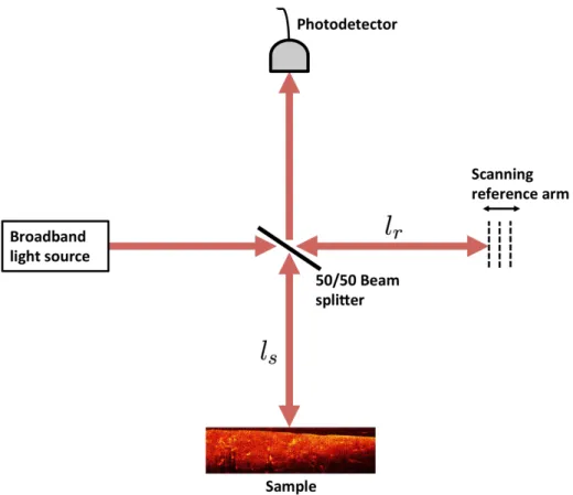
OCT was first conceived as a time-domain system (Time Domain OCT, TD-OCT)
in which the interferogram is collected by rapidly changing the optical path length
between the sample and reference beams in a Michelson interferometer [28]. Although
TD-OCT has been successfully employed to investigate many types of biological samples,
its limiting factors have been the lack of optical phase stability, and the speed of data
acquisition which is limited by the the scanning speed of the interferometer reference
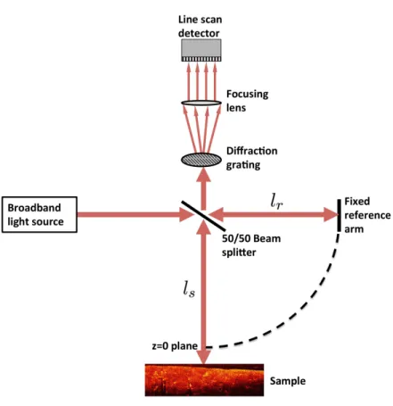
arm. These limitations of TD-OCT are overcome by systems working in the Fourier