and Optimal Control
Douglas G. Down
Department of Computing and Software McMaster University
1280 Main Street West, Hamilton, ON L8S 4L7, Canada [email protected]
905-525-9140 Mark E. Lewis
Department of Industrial and Operations Engineering University of Michigan
1205 Beal Avenue, Ann Arbor, MI 48109-2117 [email protected]
We consider a system of parallel queues with dedicated arrival streams. At each decision epoch a decision-maker can move customers from one queue to another. The cost for moving customers consists of a fixed cost and a linear, variable cost dependent on the number of customers moved. There are also linear holding costs that may depend on the queue in which customers are stored. Under very mild assumptions, we develop stability (and instability) conditions for this system via a fluid model. Under the assumption of stability, we consider minimizing the long-run average cost. In the case of two-servers the optimal control policy is shown to prefer to store customers in the lowest cost queue. When the inter-arrival and service times are assumed to be exponential, we use a Markov decision process formulation to show that for a fixed number of customers in the system, there exists a levelSsuch that whenever customers are moved from the high cost queue to the low cost queue, the number of customers moved brings the number of customers in the low cost queue toS. These results lead to the development of a heuristic for the model with more than two servers.
1
Introduction
The problem of scheduling jobs in parallel processing networks has widespread use in computer, telecom-munications, manufacturing, and even health systems. Given a set of processors, when a job (customer) arrives a decision-maker must decide where it should be served in order to maximize or minimize the given performance measure. In most models this decision must be made immediately and is thus, a routing de-cision based on the loads of each queue in the network. The customer must then wait in queue for the processor (server) to become free before receiving service. We consider a model that is quite different. Instead of a routing decision made upon arrival we allow the decision of where a customer is served to be a load balancing decision that can be made upon arrival and then adjusted at several discrete points in time. That is, suppose we again have a system of parallel queues but that each queue has a dedicated arrival stream. At some (possibly random) points in time a manager may choose to move customers in a particular queue to one of the other queues. Once this decision is made, customers move from one queue to the other with certainty and instantaneously. In this manner, a decision-maker may ensure that the load is balanced so as to avoid idleness and/or high holding costs.
The topic of load balancing in distributed systems has a vast literature, particularly in the area of mul-tiprocessor/multicomputer systems. Two general references are the monographs of Shrazi et al. [17] and Bharandwaj et al. [1]. Wang and Morris [19] provide a survey of results for several load balancing algo-rithms. These basically fall into the areas of routing (Join the Shortest Queue, etc.) and server movement (analysis of the system as a polling model). The determination of optimal routing policies to balance proces-sor loads has been studied by many authors. A representative, but by no means exhaustive, list is the work of Liu and Righter [14], Boel and van Schuppen [2], Koole [9] and Towsley et al. [18]. The additional com-plication of synchronization of parallel tasks is incorporated into the optimal scheduling problem examined in Xia et al. [20], where the control mechanism is also the routing of incoming arrivals.
Of particular relation to this paper is the work of Lewis [11], He and Neuts [8] and Levine and Finkel [10]. As has been alluded to, the usefulness of the current model over the routing models is in the fact that the balancing decision is made after the customers have been assigned to a particular queue. That is to say that in the routing model, if a long service time has caused the queues to become unbalanced, the decision-maker has no recourse but to wait until the long queue empties, while in the load balancing model we may immediately balance the load. Lewis [11] considers the single server case with two admission control decisions, one immediately before service, analogous to our load balancing decision. He and Neuts [8] consider the two-server case restricting attention to policies that move a fixed number of customers when the difference in the queue lengths reaches a certain level. Both works make the assumption of exponential inter-arrival and service times and therefore discuss policies that are based solely on the queue lengths. In the latter the authors use Foster’s criterion to show that if the total service rate is higher than the total arrival rate, the system is stable. A simple example will show that without the exponential assumption there exists reasonable policies for which this is not sufficient. The model studied here is a generalization of that in [10]: the arrival rates are allowed to be unequal and the cost structure is more general. In addition, the focus of this paper is to find the stability region and study the structure of optimal policies, whereas in [10] there is an a priori restriction to threshold policies.
We are interested in both the design and control of the load balancing system. Since control considera-tions cannot be addressed without first addressing the stability question, we discuss condiconsidera-tions under which policies yield a stable Markov chain; one for which there exists a stationary distribution. This is done with-out any distributional assumptions. We then discuss the two-server case to gain insight into the structure of an optimal control policy. Unfortunately, when the number of servers increases, making the queue length information available in real-time (for every server) is undesirable. Thus, in order to extend these results to the more general case we examine a heuristic policy based on a dynamic pairing scheme. The idea is quite simple. If a server becomes idle, it chooses a queue to be paired with and uses the optimal two-server balancing decision. This reduces the overhead required and takes advantage of the insights gained from the two-server problem.
The rest of the paper is organized as follows: We give a formal description of the model in Section 2. In Section 3 we discuss conditions under which a wide class of policies are stable. Section 4 contains the analysis of the optimal control of both the two-server andN−server models. We conclude in Section 5.
2
Problem Description
Consider a sequence ofNparallel queues. Customers arrive to queueiat times{τi
k, k≥0}such thatτ0i = 0
andσki =τki+1−τki are independent and identically distributed (iid) fori= 1, . . . , N. The corresponding arrival rate to queueiisλi = 1/Eσi1 . The service processes of each queue are independent and similarly
defined. That is, thenthcustomer that is served by serverirequiresηintime units of service where{ηi n, n≥
1, i= 1,2, . . . , N}are assumed to be iid. We assume that each server has the same service rateµ, but the underlying distributions may be different.
Let Πbe the set of all non-anticipating policies. A policy π ∈ Πprescribes how many customers to move from one queue to another, given the number of customers in each queue (the queue length process), perhaps the amount of time each customer has been in service, the time since the last arrival to each queue and any other information that is required to make the (policy dependent) process Markovian. In the most general case, all of this information is captured by the current state of the system.
The cost for moving j customers contains a fixed cost K and a variable cost mj. Furthermore, the system continuously incurs holding cost hini per unit time that queueicontainsni customers (including
the one in service). We seek to find a strategy for load balancing under the long-run average cost optimality criterion. Note here that the term “load balancing” is used somewhat loosely since the holding costs may cause the optimal policy to leave the distribution of the number of customers at each queue unbalanced. In some sense, perhaps “load distribution” would be more appropriate, but we will continue to refer to the control as balancing without further comment in hopes that it will cause no confusion.
For a fixed policy π, denote the set of decision epochs byD ≡ {ρk, k ≥ 0}and the state at the ith
decision epoch byXi. For example, if π depends only on the queue lengths, thenD is the set of arrival
times and service time completions. We assume that the time between decision epochs is bounded away from zero so that only a finite number of decisions can be made in a finite amount of time. If we let Qπ(t) = {Qπ
the notation of Puterman [13], let gπ(x) = lim sup n→∞ Eπx n Pn i=0 h k(Xi, Yi) + Rρi+1 ρi c(Xi, Yi)dt io Eπx{ρn} , (2.1)
whereYi is the action taken at decision epochi,k(·)andc(·)are the lump sum cost and cost rate of said
action, respectively, and the expectation is conditioned on the initial state of the system under the policy π. The quantitygπ(x)is called the long-run average expected cost starting in statexunder policyπ. The objective then is to find a policyπ∗such thatgπ∗(x)≤gπ(x)for all statesxand all policiesπ∈Π.
3
Stability
In this section we discuss conditions under which the system is stable. As has been alluded to, this is done in a general enough fashion so as to not require restrictive assumptions. In particular, we would like to avoid having to restrict attention to policies based solely on queue lengths or those that only redistribute customers after a fixed amount of time. The heuristic described in Section 4.3 is in fact, a hybrid of these. In order to arrive at the main results of this section, we introduce the fluid model. That is, we replace the (random) arrival and service processes by deterministic processes defined by their rates, at which point these processes can be thought of as fluid flows. Upon applying several classic results of Dai [3] we arrive at the conditions for the stability of the load balancing network. We then extend these results to show that under the same conditions derived for stability, we can guarantee the finiteness of the average cost.
3.1 System Dynamics
For the remainder of this section, fix an arbitrary policy π ∈ Π. In order to simplify notation for the quantities defined, we suppress dependence on this policy. For each j = 1,2, . . . N, let Ej(t) be the
number of exogenous customers arriving to queuejin(0, t]. LetSj(t)be the potential number of service
completions by serverjin(0, t]. That is to say thatSj(t)is the number of service completions that would
occur if there were no idling of serverj. LetAj(t) be the residual arrival time at timetfor streamjand
let Bj(t)be the residual service time at server j. For convenience assume that Aj(t)andBj(t) are right
continuous forj= 1, . . . , N. Thus, we have
Ej(t) = max{n≥0 :Aj(0) +σj1+· · ·+σ j n−1 ≤t}, Sj(t) = max{n≥0 :Bj(0) +ηj1+· · ·+η j n−1≤t},
where the maximum of an empty set is defined to be zero. LetTj(t)be the cumulative busy time for server
jin(0, t]. The evolution of the total number in the system,M(t), is thus given by
M(t) =M(0) + N X j=1 Ej(t)− N X j=1 Sj(Tj(t)). (3.1)
The functionsTj(t)are determined by the control policyπ. Recall thatπis assumed to be non-anticipating
and thatQj(t)is the number of customers in queuejat timet. Define
where (Dk(t), k = 1, . . . , Ns) is an Ns-dimensional vector chosen such that X(t) is a Markovian state
evolving on the state spaceX=ZN+×RN+×RN+×RN+s and the processXhas the strong Markov property.
For example, if π is a policy such that decision epochs are spaced a constant, td, time units apart and
decisions are made based on the queue length and residual time information, thenNs = 1 andD1(t) is
the elapsed time since the last decision. If the inter-arrival and service times are exponential, residual time information is not necessary.
3.2 Stability of fluid models
Letq=M(0). Suppose that the function( ¯M(·),T¯j(·) :j= 1, . . . , N)is a limit point of
(q−1M(qt), q−1Tjq(qt) :j= 1, . . . , N)
whenq→ ∞, where the dependence ofTjqonqhas been added for clarification. When it exists( ¯M(t),T¯j(t) :
j= 1, . . . , N)is called a fluid limit of the system. Since we have been able to describe the system dynamics in the form (3.1), Dai [4, Theorem 2.3.2] yields that a fluid limit exists (it may not be unique). Furthermore, each of the fluid limits is a solution of the following set of conditions, known as the fluid model.
¯ M(t) = M¯(0) + N X j=1 λjt−µ N X j=1 ¯ Tj(t); (3.2) ¯ M(t) ≥ 0, (3.3) ¯
Tj(0) = 0andT¯j(·)is non-decreasing forj = 1, . . . , N. (3.4)
As has previously been alluded to, (3.2) is a deterministic version of (3.1) with the arrival and service processes replaced by their rates.
The fluid model is said to be stable if there exists a fixed time t0 such thatM¯(t) = 0, for allt ≥ t0,
for any fluid solution. The fluid model is said to be unstable if for every solution of the fluid model with ¯
M(0) = 0, there exists aδ >0such thatM¯(δ)6= 0. Thus, stability of the fluid model states that eventually all queues will drain, and once drained, they remain empty.
Suppose that the following condition holds:
P1. For allt >0, there existsε >0such that with probability one,
lim q→∞ N X j=1 Tjq(t)≥ PN j=1λj µ +ε ! t−δ for someδ <∞.
Since a fluid limit is defined as q approaches infinity, for q sufficiently large, P1 ensures that for all but a finite amount of time, the servers are working at a rate greater than the total arrival rate. Under P1 the stability of the system is almost immediate (shown momentarily).
Proposition 3.1 (i) IfPNj=1λj < N µ, then for any control policyπsatisfying P1, the fluid model is stable
and, thus, an invariant probabilityϕexists forX.
Proof. (i) From P1, PNj=1dtdT¯j(t) ≥ ε+PNj=1λj/µforj = 1, . . . , N. Examining (3.2) we have that
¯
M(t) = 0for allt≥M(0)/ε. Thus the fluid model is stable, and the existence of an invariant probability forXfollows from Theorem 4.2 of Dai [3].
(ii) We havePNj=1 dtdT¯j(t)<PNj=1λj/µ, which implies that ifM¯(0) = 0,M¯(1)≥PNj=1λj −N µ >0,
so the fluid model is unstable. The transience ofXfollows from Theorem 2.5.1 of Dai [4].
Although P1 is intuitive, it may be a bit unwieldy to verify. One might think that instead, we could assume that all servers are busy when the number of customers reaches a certain level. This would ensure that all of the capacity is eventually used. If this capacity is greater than the arrival rate, we again arrive at stability conditions. This is captured by the following alternative to P1.
P1’. For someTM >0,M(t)≥TM ≥N ensures that all servers are busy at timet.
It is easy to see that if P1’ holds, P1 holds withε=N −PNj=1λj/µ >0andδ = 0. That is, P1’ is more
restrictive than P1. The next two examples illustrate policies that satisfy P1’.
Example 3.2 Suppose the holding cost rate of serverN is the smallest. Consider the policy that immedi-ately routes customers that arrive to find their respective server busy to serverN. Also, if server 1 through N −1becomes idle, a waiting customer at queueN (if any) is moved to the idle server. This satisfies P1’ withTM =N. Furthermore, it has the desirable properties that it reduces idling and takes advantage of the
fact that queueN has the smallest holding cost.
Example 3.3 Consider the policy that moves customers only to avoid idling. If queue j becomes idle, a waiting customer is moved from the queue where hjQj(t) is maximized; ties broken arbitrarily. This
satisfies P1’ withTM =N.
Unfortunately, in general, P1’ may be too restrictive. That is to say, it may not be necessary to require servers to be busy for all timest. Equally perplexing is the fact that for a large number of customers in the system P1’ requires the decision-maker to keep queue length information for each queue (or at least signal when a queue is empty). We have already discussed the pitfalls of this proposition. The next example illustrates a simple class of policies that might be useful but that do not satisfy P1’.
Example 3.4 Suppose that everytdtime units, the policy equalizes the number of customers in each queue
(to within one customer). Then P1’ does not hold, but P1 holds withε=N −PNj=1λj/µandδ =N td.
We conclude our discussion of stability with a counterexample to the conjecture that the assumption that
PN
j=1λj < N µis enough to guarantee stability in general. Recall, this inequality was shown to be sufficient
in the exponential case in [8].
Example 3.5 Consider a policy with periodic arrivals and deterministic service times, withN = 2,λ1 =
6.5,λ2 = 0.5, andµ= 5. Everytd= 1time units, one customer is moved from queue 1 to queue 2. Ifqis
chosen such thatQ1(0)→ ∞andQ2(0) = 0, then
N X
j=1
This violates P1 and Proposition 3.1 part (ii) yields that the policy is unstable. To stabilize the system, either the decision epochs need to be more closely spaced, or more customers must be moved at each decision epoch.
From a design standpoint, stability is a necessary consideration. To facilitate the control question, we begin by restricting attention to policies that yield finite average cost. To this end, we make the following additional assumptions.
M1. The interarrival and service times have finite second moments, i.e. E[(σj1)2]<∞andE[(η1j)2]<∞
forj= 1, . . . , N.
Theorem 3.6 Ifπsatisfies P1, the system satisfies M1 andPNj=1λj < N µ, thengπ(x)<∞for allx∈X.
Proof. Under P1, Proposition 3.1 (i) implies that the fluid model is stable. Stability of the fluid model and M1 allow us to apply Theorem 4.1 of Dai and Meyn [5], which in turn implies
lim
t→∞Ex[Qj(t)] =Eϕ[Qj(0)]<∞.
From this, we also conclude that the mean time spent in the system by a customer from any stream j, limt→∞E[Wj(t)], is finite. The average cost can be broken into two parts; that due to the holding costs and
that due to the switching costs. The portion due to the holding costs can be written,
lim t→∞ N X j=1 hjEx[Qj(t)]<∞.
By assumption, the expected number of decision epochs that occur while a customer is in the system is also finite. Thus, the part of the average cost due to switching costs per unit time is finite and the result is proven.
4
Optimal Control
In this section we discuss the optimal control of the load balancing network. It should be clear that as the number of servers grows the size of the state space becomes intractable. In fact, even in the case withN = 2, without any distributional assumptions the state space is uncountable since (at the very least) the residual arrival and service times must be included. Our approach is thus to consider the two-server model and prove what we can about the structure of an optimal control policy in this case. We then take the insights gained from this model and develop a heuristic for control of the generalN−server model. Unless otherwise stated for the remainder of the paper we assume P1 and M1 hold and thatPNj=1λj < N µ.
4.1 The Two-server model
In this section we study the model whenN = 2in an attempt to understand more fully motivations for optimal control in the more general case. Under various assumptions we discuss the structure of an optimal
control policy. The main point that should become obvious in this section is that the load balancing decision should incorporate the desire to empty the system as quickly as possible and the need to do so at minimal cost. Without loss of generality we assume (unless otherwise stated) thath1≥h2. The first result states that
one should not move customers to a higher cost queue except possibly to avoid idling.
Theorem 4.1 Supposeh1 ≥h2, then there exists an optimal policy that moves customers from queue 2 to
queue 1 only when queue 1 is empty.
Proof. The result is proved by a sample path argument. Consider two processes defined on the same probability space so that each sees the same sequence of inter-arrival times and service times. Denote the first process by{Y(t) = (Q1(t), Q2(t)), t ≥0}. This process uses a policyπ that calls for movingk > 0
customers from queue 2 to queue 1 whenY(t) = (i∗, j∗),i∗>0where(i∗, j∗)is assumed to have positive probability of being reached during the cycle. The second process,{Y0(t) = (Q01(t), Q02(t)), t ≥ 0}uses the policyπ0, which is identical toπ with the exceptions detailed below. To specify these exceptions, we need some additional notation. Each process begins at(0,0). For simplicity, if t∗ is a decision epoch we letπ(t∗) = κ > 0when the policy calls for movingκcustomers from queue 1 to queue 2. Similarly, let π(t∗) =κ <0when the policy calls for movingκcustomers from queue 2 to queue 1. Let
α= inf{t≥0|Y(t) =Y0(t) = (i∗, j∗), π(t)>0} β = inf{t≥α|Y0(t) = (0, j)for somej≥0} γ = inf{t≥α|π(t)>0}
δ = inf{t≥α|Y(t) = (i,0), π(t) = 0for somei≥0}
where the infimum of the empty set is taken to be infinite.
We now complete the description of π0. At timeα, π0 does not move any customers from queue 2 to queue 1. Thus, Y(α) = (i∗ +k, j∗ −k) andY0(α) = (i∗, j∗). Suppose first thatδ < γ ≤ β so that Y(t) = (i,0)whileQ02(t) ≥ k. Thenπ0(δ)moves kcustomers from queue 2 to queue 1. The processes couple and the costs afterδare the same. The difference in the total costs on the cycle is
D0 ≡k(δ−α)(h1−h2)≥0.
Supposeγ < δ ≤β orγ ≤β < δ. That is,π calls for moving customers from queue 1 to queue 2 before Q01(t) = 0 or Q2(t) = 0. Then π0 moves only enough customers to queue 1 so that the two processes
coincide, after which,π0(t) = π(t)for all t > γ. The processes are then coupled and the costs thereafter on the cycle are the same. For example, ifπ(γ) = `(move `customers from queue 1 to queue 2), then π0(γ) =k−`. The difference in the total cost on the cycle is
D1 ≡k(γ−α)(h1−h2) + (2K+mk+m`)−(K+m|`−k|)>0,
where the first term defines the difference in the holding costs for having heldkmore customers in queue 1 underπthanπ0. The remaining terms represent the difference in having to make 2 load balancing decisions under policyπand only 1 underπ0.
Ifβ ≤γ < δorβ ≤ δ < γ, thenQ01(β) = 0,Q02(β) ≥kandQ1(β) =k. At this point,π0 calls for
movingkcustomers from queue 2 to queue 1;π0(β) = k. The processes again are coupled and the costs thereafter are the same. The difference in total cost on the cycle in this case is
D2 ≡ k(β−τ)(h1−h2)≥0.
In each case the total cost underπ0is less than that underπ. Furthermore, since the cycle times are the same, the average cost under policyπ0is less than that underπ. Sinceπ was an arbitrary policy that moves work from queue 2 to queue 1 wheni∗>0the proof is complete.
We make several remarks that are apparent from the previous theorem. Notice that the proof of Theo-rem 4.1 does not depend on the arrival processes. Thus, using symmetry, ifh1 =h2then there is no need to
move customers from one queue to another unless one is empty. Consider now the case whenh1 > h2and
m=K = 0. Theorem 4.1 implies that we need not move customers from queue 2 to queue 1 unless queue 1 is empty. It is simple to see that if we move more than one customer, the holding cost is higher than if we had only moved one, yet the system is still working at the same rate (2µ). Since moving customers does not cost anything, the average cost on any sample path is higher. Similarly, arriving customers to queue 1 can be “stored” in queue 2 at a lower cost so that (at least) all but one of these customers should be moved to queue 2. That is, when there are no switching costs, the high cost queue is only used to avoid idling. If in addition to zero switching costs there is no high cost queue (h1=h2), then any non-idling policy is optimal.
Finally consider the symmetric case with zero variable switching costs;h1 =h2,λ1 =λ2andm = 0.
The previous remarks yield that we need not move customers unless one of the queues is empty. Further-more, since the arrival rates are the same, when they are non-empty, both queues drain at the same rateµ. If the decision is made to move customers, to avoid having to balance the load frequently, one should move precisely half of the customers.
We collect all of the ideas of the previous discussion in the next proposition. Since the methods of proof have already been outlined we omit proofs, but they follow from sample path arguments similar to that in Theorem 4.1.
Proposition 4.2 In the two-server problem if
1. h1 =h2(equal holding costs), then there exists an optimal policy such that customers are moved from
one queue to another only to avoid idling.
2. m = K = 0(no switching costs), then there exists an optimal policy such that there is never more than one customer in the queue with the highest holding cost.
3. m=K = 0andh1 =h2, then any non-idling policy is optimal.
4. m = 0,h1 = h2 andλ1 = λ2, then there exists an optimal policy that when customers are moved
4.2 The Exponential Case
In this section we assume that the inter-arrival and service times are exponential. We note that this assump-tion allows the interpretaassump-tion that customers actually arrive to a router in accordance with a Poisson process of rateαsay, and that a customer is routed to queueiwith probabilityλi/αfori= 1,2. The system
dynam-ics for this model are the same as that in He and Neuts [8], the difference in our model is that the optimality criterion is quite different and we make no a priori restrictions to a particular class of policies. Of course, since the exponential assumption has been made, the stability conditions only require thatλ1 +λ2 < 2µ.
For the remainder of this section assume that uniformization has been applied in the spirit of Lippman [12] with uniformization constantΨ≡λ1+λ2+ 2µ. Without loss of generality we assumeΨ = 1so that the
arrival and service rates can be interpreted as probabilities. Thus, instead of considering the continuous-time load balancing problem, we consider a discrete-time equivalent.
We develop a Markov decision process describing the average cost problem. We then further charac-terize the optimal policies by considering the structure of policies that achieve the minimum in the average cost optimality equations (ACOE), and are thereby average cost optimal. We first state the ACOE for our model. Let(I, i)∈ {(k, `)∈Z+
×
Z+|k≥`} ≡X, where the first element represents the total number of
customers in the system and the second element represents the number of customers in queue 2 (the low-cost queue). The ACOE fori≤Iare
g+h(I, i) = min
a∈{−i,...,I−i}{K1{a6=0}+m|a|+ (I−i−a)h1+ (i+a)h2+U(I, i+a)}, (4.1) where
U(I, i) =λ1h(I+ 1, i) +λ2h(I+ 1, i+ 1) +µ h((I−1)+, i) +µ h((I−1)+,(i−1)+).
It is well-known that if(g, h)satisfies (4.1) theng =g∗ ≡infψ∈Πgψ andh(often called a relative value
function) is unique up to a constant. The fact that a solution to the ACOE exists follows from Theorem 3.6 and results in Meyn [15, Theorems 3.1, 5.1-2]. For brevity we simply note that the proof requires that the policy improvement algorithm is initialized with a policy with finite average cost. Since existence of such a policy is guaranteed by Theorem 3.6 the algorithm converges to a solution of the ACOE. The next result follows directly from the ACOE, but simplifies the search for an optimal policy considerably.
Proposition 4.3 Suppose that there areI customers in the system. There exists anS(I)≤Isuch that 1. the optimal policy does not move customers fori > S(I)and
2. when customers are moved from the high to the low cost queue the number of customers in the low cost queue isS(I).
The conspicuous use of “S” in Proposition 4.3 is not accidental. The result states that the optimal policy is an order-up-to policy analogous to(s, S)policies in inventory control models. That is to say that ifi < S(I), and it is optimal to move customers, then it is optimal to bring the number of customers in queue 1 up to S(I).
Proof. For0≤i≤I let
G(I, i)≡mi+ (I−i)h1+ih2+U(I, i).
The ACOE can be rewritten fori < I
g+h(I, i) = min{G(I, i), min
a∈{−i,...,I−i}/{0}{K+ 2ma −
+G(I, i+a)}} −mi, (4.2)
where the superscript “−” represents the negative part ofa. Using the change of variablesb=i+a, (4.2) becomes g+h(I, i) = min{G(I, i), min b∈{0,...,I}/{i}{K+ 2m(b−i) − +G(I, b)}} −mi. Let S(I)∈argmin{b∈ {0, . . . , I}/{i} |2m(b−i)−+G(I, b)}.
Then directly from the ACOE we note that the optimal policy moves customers to make the number of customers in the low cost queue S(I) when K + 2m(S(I) −i)− +G(I, S(I)) < G(I, i), moves no customers when the reverse inequality holds and is indifferent when equality holds. Furthermore, the results of Theorem 4.1 state that we need not move customers whenI > i > S(I)since that would entail moving customers from the low cost queue to the high cost queue when the high cost queue is not empty. Thus, the result is proven.
One might note that Proposition 4.3 does not eliminate from consideration the policy that does not move customers in state(I, i), yet moves customers in state(I, i+ 1), where (i+ 1< I). We conjecture that there exists an optimal policy that does not have this property. Indeed our numerical studies have confirmed this conjecture, but we have not been able to prove it to date.
This section has yielded several insights. There are in essence two questions that we have tried to answer:
• When should we move customers?
• When customers are to be moved, how many customers should be moved?
The first question is addressed in Theorem 4.1 and Proposition 4.2. The intuition is simple, we should move customers to avoid idling with the restriction that we would also like to have most of the customers in the lower cost queue. When these concerns are alleviated, several special cases arise.
The second question above is discussed in the context of the exponential assumptions. Under these as-sumptions the existence of an optimal policy that is analogous to the order-up-to policies found in inventory control is shown. That is, for each fixed number of customers in the system, when customers are to be moved, there is a number of customers in the low cost queue that it is optimal to meet. This of course is tempered by the fact that we do not move customers from the low cost to the high cost queue unless the high cost queue is empty. In the next section we attempt to apply these insights to the more general case with any finite number of servers.
4.3 TheN−server model
The results of the previous two sections give insight into how to design policies for systems with more than two servers. Unfortunately, implementing some of these ideas on a general network is undesirable due to the amount of information that must be provided to each processor. On the other hand, since we are able to construct simple optimal policies for two-server systems, we suggest a set of policies in which an idle server probes others one at a time. The optimal two-server policy is used to decide the number of customers to move. If no customers are moved, the server probes another queue. The advantage to this simple, scalable set of policies is that there is a minimal amount of communication overhead, while maintaining a connection to our previous results.
For simplicity, assume equal holding costs, i.e. hi = 1, i = 1, . . . , N. Our policy is (informally)
described as follows:
1. When queueiempties, (randomly) choose another queuej.
2. Perform a transfer from queue j to queue iaccording to the optimal policy for the corresponding two-server system.
3. If no transfer takes place, choose another queuejthat has not previously been selected. Repeat steps two and three until either a transfer is made or until all queues have been examined.
4. If queueiremains empty after this procedure, wait until a customer arrives to queueior until some fixed timeT elapses. Return to step one.
The inspiration for our policy is a similar idea for a routing problem suggested in the work of Eager, La-zowska and Zahorjan [7].
This set of policies has several desirable properties. First, decisions are made only at emptying times, which from Part 1 of Proposition 4.2 appears to be a reasonable choice. Second, a server does not need to know the queue lengths at all of the other servers. These first two properties result in low communication overhead. Once this communication is made, guidelines on how many customers should be moved, can be obtained from the results of Section 4.2 and in special cases, the remaining results of Propositions 4.2. In the exponential case, the order-to-levels can be stored in a one-dimensional array for easy look up. Finally, the policy is stable as P1’ is satisfied for allt≥ T. This of course is crucial as a priori there is no need to believe a particular non-idling policy is stable.
To illustrate how this policy performs, we simulated a system with six servers, with arrival ratesλ1 =
.75,λ2 = .9, λ3 = .85,λ4 = 1.10, λ5 = λ6 = .8. The service rateµwas set to one and we varied the
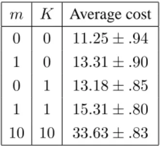
switching costs. All inter-arrival and service times were assumed exponential. In implementing the policy, the choice of which server to examine made by an idle server was done so randomly (uniform). The time an idle server would wait before probing again wasT = 10,000time units. This implies that in step 4, a queue that is empty after probing all other queues always waits until a customer arrives before returning to step 1. We still get excellent performance with this conservative choice. The design ofTis left as a topic for future research. The simulations were run using 30 replications of length 10,000 time units. The resulting 95 percent confidence intervals for the mean cost are given in Table 1.
m K Average cost 0 0 11.25±.94 1 0 13.31±.90 0 1 13.18±.85 1 1 15.31±.80 10 10 33.63±.83
Table 1: Simulation results for a six-server system
The results are quite promising, indicating that policies of this form merit further detailed study. Note that the original system would be unstable if no control were used. For them=K = 0case, a benchmark would be an M/M/6 system, which yields an average cost of 9.50. The difference is due to the large value of T. It is not difficult to see that asT decreases, the behaviour would approach that of an M/M/6 system. The choice ofT thus involves a tradeoff between performance and overhead. Finally, when the costs increase by a factor of 10, the resulting overall cost roughly doubles, indicating that the proposed policy may be particularly useful in the face of high switching costs.
5
Conclusions
In this paper we have examined a method for dynamically balancing the load in parallel processing networks. We showed that in order to cover a larger class of policies, the assumptions implied by the exponential case are not sufficient. The fluid model opens the door to policies that are based on queue length, time since the last decision and/or those that are some hybrid of the two.
For control, we used a “divide and conquer” approach that is usual in operations research practice. By examining the model with only two servers, we gain valuable insights into the structure of an optimal policy in theN−server system. In particular, we note that when the switching costs are small, and the holding costs equivalent, the main concern is to avoid idling. In this case, a non-idling policy seems sufficient, but at the cost of an inordinate amount of overhead. In order to alleviate this difficulty, we discuss a simple policy that attempts to minimize idleness, but does so in a “smart” way, which allows us to exploit the optimal two-server policy. This is quite simple when we have equal holding costs. In a more complicated system, we may want to move customers to the low-cost queue before it becomes empty. This complicates our heuristic somewhat, and provides an interesting challenge for future research.
In our numerical results, an idle server chose the next server to pair with uniformly. One extension may be that each server keeps information about the last state of the queues probed and uses this information to decide which queue to pair with next. This and other extensions will be undertaken in subsequent research.
6
Acknowledgements
The authors would like to thank Marcel Neuts for originally suggesting this model. We would also like to thank Eugene Feinberg of the State University of New York at Stony Brook for finding a mistake in an
earlier version of this paper and Robert D. Foley of the Georgia Institute of Technology for suggesting that we consider the total number of customers in the state space. The work of the first author is supported by the Natural Sciences and Engineering Research Council of Canada. The work of the second author is partially supported by the National Science Foundation grant DMI-0132811.
References
[1] V. Bharadwaj, D. Ghose, V. Mani and T.G. Robertazzi. Scheduling Divisible Loads in Parallel and Distributed Systems. IEEE Press, 1996.
[2] R.K. Boel and J.H. van Schuppen. Distributed routing for load balancing. Proceedings of the IEEE, 77:210–221, 1989.
[3] J.G. Dai. On positive Harris recurrence of multiclass queueing networks: a unified approach via fluid limit models. Annals of Applied Probability, 5:49-77, 1995.
[4] J.G. Dai. Stability of Fluid and Stochastic Processing Networks. MaPhySto Miscellanea no. 9, 1999.
[5] J.G. Dai and S.P. Meyn. Stability and convergence of moments for multiclass queueing networks via fluid models. IEEE Transactions on Automatic Control, 40:1889-1904, 1995.
[6] M.H.A. Davis. Piecewise deterministic Markov processes: a general class of diffusion stochastic models. Journal of Royal Statistic Society, Series B, 46:353-388, 1984.
[7] D.L Eager, E.D. Lazowska and J. Zahorjan. Adaptive Load Sharing in Homogeneous Distributed Systems. IEEE Transactions on Software Engineering, SE-12:5:662-675, 1986.
[8] Q. He and M.F. Neuts. Two M/M/1 Queues with transfer of customers Queueing Systems 42:377–400, 2002.
[9] G. Koole. On the pathwise optimal Bernoulli routing policy for homogeneous parallel servers. Math-ematics of Operations Research, 21:469–476, 1996.
[10] A. Levine and D. Finkel. Load balancing in a multi-server queueing systems. Computers Opns Res., 17:17-25, 1990.
[11] M.E. Lewis. Average optimal policies in a controlled queueing system with dual admission control. Journal of Applied Probability, 38:2:369-385, 2001.
[12] Lippman, S. Applying a New Device in the Optimization of Exponential Queueing System. Operations Research, 23:687-710, 1975.
[13] M.L. Puterman. Markov Decision Processes: Discrete Stochastic Dynamic Programming. John Wiley and Sons, Inc., New York, 1994.
[14] Z. Liu and R. Righter. Optimal load balancing on distributed homogeneous unreliable processors. Operations Research, 46:563–573, 1998.
[15] Meyn, S. The Policy Improvement Algorithm for Markov Decision Processes. IEEE Transactions on Automatic Control, 42:12:1663 -1680, 1997.
[16] L.I. Sennott Stochastic dynamic programming and the control of queueing systems. John Wiley and Sons, Inc., New York, 1999.
[17] B.A. Shirazi, A.R. Hurson and K.M. Kavi. Scheduling and Load Balancing in Parallel and Distributed Systems. IEEE Press, 1995.
[18] D. Towsley, P.D. Sparaggis and C.G. Cassandras. Optimal routing and buffer allocation for a class of finite capacity queueing systems. IEEE Transactions on Automatic Control, 37:1446–1551, 1993.
[19] Y-T Wang and R.J.T. Morris. Load sharing in distributed systems. IEEE Transactions on Computers, 34:204–217, 1985.
[20] C.H. Xia, G. Michailidis and N. Bambos. Dynamic on-line task scheduling on parallel processors. Performance Evaluation, 46:219–233, 2001.