Precomputing Interactive Dynamic
Deformable Scenes
Doug James Kayvon Fatahalian
Abstract
We present an approach for precomputing data-driven models of interactive physically based deformable scenes. The method permits real-time hardware synthesis of nonlinear deformation dynamics, including self-contact and global illumination effects, and supports real-time user interaction. We use data-driven tabulation of the system's deterministic state space dynamics, and model reduction to build efficient low-rank parameterizations of the deformed shapes. To support runtime interaction, we also tabulate impulse response functions for a palette of external excita-tions. Although our approach simulates particular systems under very particular interaction conditions, it has several advantages. First, parameterizing all possible scene deformations enables us to precompute novel reduced coparam-eterizations of global scene illumination for low-frequency lighting conditions. Second, because the deformation dynamics are precomputed and parameterized as a whole, collisions are resolved within the scene during precom-putation so that runtime self-collision handling is implicit. Optionally, the data-driven models can be synthesized on programmable graphics hardware, leaving only the low-dimensional state space dynamics and appearance data models to be computed by the main CPU.
Contents
1 Introduction 1
1.1 Related Work 2
2 Data-Driven Deformation Modeling 3
2.1 Deterministic State Space Model 3
2.2 Data-driven State Spaces 3
2.3 Dimensional Model Reduction 4
2.3.1 Model Reduction Details 4
2.3.2 Reduced State Vector Coordinates 4
3 Dynamics Precomputation Process 5
3.1 Data-driven Modeling Complications 5
3.2 Impulse Response Functions 5
3.3 Impulse Palettes 6
3.4 Interaction Modeling 7
3.5 Impulsively Sampling the Phase Portrait 7
4 Reduced Global Illumination Model 8
4.1 Radiance Transfer for Low-frequency Lighting 8
4.2 Dimensional Model Reduction 8
4.3 Interpolating Sparsely Sampled Appearances 9
5 Runtime Synthesis 9
5.1 Approximating Impulse Responses 9
5.2 Caching Approximate IRF References 10
5.3 Low-rank Model Evaluation 10
6 Results 10
7 Summary and Discussion 12
A Output-Sensitive SVD 13
B NRBF Appearance Interpolation 14
1 Introduction
Deformation is an integral part of our everyday world, and a key aspect of animating virtual creatures, clothing, frac-tured materials, surgical biomaterials, and realistic natural environments. It also constitutes a special challenge for real-time interactive environments. Designers of virtual environments may wish to incorporate numerous deformable components for increased realism, but often these simulations are only of secondary importance so very limited com-puting resources are available. Unfortunately, many realistic deformable systems are still notoriously expensive to simulate; robustly simulating large-scale nonlinear deformable systems with many self-collisions is fundamentally expensive [BFA02], and doing so with real-time constraints can be onerous. Perhaps as a consequence, very few (if any) major video games have appeared for which complex deformable physics is a substantial component. Numerous self-collisions complicate both runtime simulation and precomputation of interesting deformable scenes, and are also a hurdle for synthesizing physical models in real-time graphics hardware. Finally, realistic real-time animation of global illumination effects is also very expensive for deformable scenes, largely because it can not be precomputed as easily as for rigid models.
The goal of this paper is to strike a balance between complexity and interactivity by allowing certain types of interactive deformable scenes, with very particular user interactions, to be simulated at minimal runtime costs. Our method tabulates state space models of the system's deformation dynamics in a way that effectively allows interactive dynamics playback at runtime. To limit storage costs and increase efficiency, we project the state space models into very low-dimensional spaces using least-squares (Karhunen-Loeve) approximations motivated by modal analysis. One might note that the highly complex geometry of dynamical systems' phase portraits, even for modest systems, suggests that it may be impractical to exhaustively sample the phase portrait [GH83, AS92]. Fortunately, this is unnecessary in our case. Our goal is not to exhaustively sample the dynamics to a specified accuracy, nor build a control system, instead we wish only to plausibly animate orbits from the phase portrait in a compelling interactive fashion. To this end, we sample the phase space dynamics using parameterized impulse response functions (IRFs) that have the benefit of being directly "playable" in a simulation provided the system is excited in similar contexts. We use small catalogues of interactions defined in discrete impulse palettes to constrain the range of user interaction, and thus reduce the effort required to tabulate system responses. This diminished range of interaction and control is a trade-off that can be suitable for virtual environments where interaction modalities are limited.
A major benefit of precomputing a reduced state space parameterization of deformable shapes is that we can also precompute a low-rank approximation to the scene's global illumination for real-time use. To address realistic appear-ance modeling we build on recent work by Sloan, Kautz and Snyder [SKS02] for radiappear-ance transfer approximations of global illumination for diffuse interreflections in low-frequency lighting environments. Data reduction is performed on the space of radiance transfer fields associated with the space of deformable models. The final low-rank deformation and transfer models can then be synthesized in real-time in programmable graphics hardware as in [JP02a, SKS02].
(a) Precomputation (b) Reduced dynamics model (c) Reduced illumination model (d) Real-time simulation Figure 1: Overview of our approach: (a) Given a deformable scene, such as cloth on a user-movable door, we precom-pute (impulsive) dynamics by driving the scene with parameterized interactions representative of runtime usage, (b) Model reduction on observed dynamic deformations yields a low-rank approximation to the system's parameterized impulse response functions, (c) Deformed state geometries are then sampled and used to precompute and coparam-eterize a radiance transfer model for deformable objects, (d) The final simulation responds plausibly to interactions similar to those precomputed, includes complex collision and global illumination effects, and runs in real time.
1.1 Related Work
Deformable object simulation has had a long history in computer graphics, and enormous progress has been made [Wei86, TPBF87, PW89, BW98, OH99, BFA02]. More recently, attention has been given to techniques for interactive sim-ulation, and several approaches have appeared that trade accuracy for real-time performance. For example, adaptive methods that exploit multiscale structure are very effective [DDCB01, GKS02, CGC+02, JPO3].
In this paper we are particularly interested in data-driven precompution for interactive simulation of deformable models. Prior work includes Green's function methods for linear elastostatics [CDA99, JP99, JPO3], and modal anal-ysis for linear elastodynamics [PW89, Sta97, JP02a]. These methods offer substantial speedups, but unfortunately do not easily generalize to more complex, nonlinear systems (although see [JPO2b, KJP02] for quasistatic articulated models).
Dimensional model reduction using the ubiquitous principal component analysis (PCA) method [NelOO] is closely related to shape approximation methods used in graphics for compressing time-dependent geometry [Len99, AMOO] and representing collections of shapes [BV99, SIC01]. For deformation, it is well-known that dimensional model reduction methods based on least-squares (Karhunen-Loeve) expansions yield optimal modal descriptions for small vibrations [PW89, Sha90], and provide efficient low-rank approximations to nonlinear dynamical systems [Lum67]. We use similar least-squares model reduction techniques to reduce the dimension of our state space models. Finally, online data-reduction has been used to construct fast subspace projection (Newmark) time-stepping schemes [KLM01 ], however our goal is to avoid runtime time-stepping costs entirely by tabulating data-driven state space models using IRF primitives.
Our work is partly motivated by programmable hardware rendering of physical deformable models using low-rank linear superpositions of displacement fields. Applications include morphable models, linear modal vibration mod-els [JP02a], and data-driven PCA mixture modmod-els for character skinning [KJP02]. Key differences are that (a) we address complex nonlinear dynamics with self-collisions, and (b) our appearances are based on low-rank approxima-tions to radiance transfer fields instead of surface normal fields.
Data-driven tabulation of state space dynamics is an important strategy for identifying and learning how to control complex nonlinear systems [NelOO]. Grzeszczuk et al. [GTH98] trained neural networks to animate dynamical models with dozens of degrees of freedom, and learned the influence of several control parameters. Reissell and Pai [RP01] trained collections of autoregressive models with exogenous inputs (ARX models) to build interactive stochastic sim-ulations of a candle flame silhouette and a falling leaf. In robotics, Atkeson et al. [AMS97] avoid the difficulties and effort of training a global regression model, such as neural networks or ARX models. Instead they use "locally weighted learning" to locally interpolate state space dynamics and control data, and only when needed at runtime, i.e., lazy learning. Our data-driven state space model differs from these three approaches in several ways. Most notably, our method sacrifices the quality of continuous control in favor of a simple discrete (impulsive) interaction. This allows us to avoid learning and (local) interpolation by using sampled data-driven IRF primitives that can be directly "played back" at runtime; this permits complex dynamics, such as nonsmooth contact and self-collisions, to be easily repro-duced and avoids the need to generalize motions from possibly incomplete data. The simple IRF playback approach also avoids runtime costs associated with state model evaluation, e.g., interpolation. Another major difference is that our method uses model reduction to support very large dynamical systems with thousands or millions of degrees of freedom. Data-reduction quality can limit the effectiveness of the approach for large systems, but more sophisticated data compression techniques can be used. Finally, our state space model includes global illumination phenomena.
Our blending of precomputed orbital dynamics segments is related to Video Textures [SSSEOO], wherein segments of video are rearranged and pieced together to form temporally coherent image sequences. This is also related to synthesis of character motions from motion capture databases using motion graphs [KGP02, LCR+02]. Important
differences are that our continuous deformable dynamics and appearance models can have a potentially much larger state space dimensionality, and the physical nature of data reduction is fundamentally different than, e.g., character motion. Also, the phenomena governing dynamic segment transitions are quite different, e.g., impulse responses can result in discontinuous transitions, and we are not concerned with the issue of control, so much as physical impulse resolution.
Global illumination and physically based deformation are historically treated separately in graphics. This is due in part to the fact that limited rendering precomputations can be performed, e.g., due to changing visibility. Consequently, real-time model animation has benefitted significantly from the advent of programmable graphics hardware [LJM01] for general lighting models [POAU00, PMTH01, OHHM02], stenciled shadows [EK02], ray tracing [PBMH02], inter-active display of precomputed global illumination models [HeiOl], and radiance transfer (for rigid models) [SKS02].
Our contribution: In this paper we introduce a precomputed data-driven state space modeling approach for
gen-erating real-time dynamic deformable models using black box offline simulators. This avoids the cost of traditional runtime computation of dynamic deformable models when not absolutely necessary. The approach is simple yet ro-bust, can handle nonlinear deformations, self-contact, and large geometric models. The reduced phase space dynamics model also supports the precomputation and data reduction of complex radiance transfer global illumination models for real-time deformable scenes. Finally, the data-driven models allow dynamic deformable scenes to be compiled into shaders for (future) programmable graphics hardware.
Scope of Deformation Modeling: Our approach is broadly applicable to modeling deformable scenes, and can handle various complexities due to material and geometric nonlinearities, nonsmooth contact, and models of very large size. Given the combined necessity of (a) stationary statistics for model reduction and (b) sampling interactions for typical scenarios, the approach is most appropriate for scenes involving physical processes that do not undergo major irreversible changes, e.g., fracture. Put simply, the more repeatable a system's behavior is, the more likely a useful representation can be precomputed. Our examples involve structured, nonlinear, viscoelastic dynamic deformation; all models are attached to a rigid support, and reach equilibria in finite time (due to damping and collisions).
2 Data-Driven Deformation Modeling
At the heart of our data-driven simulator is a strategy for replaying appropriate precomputed impulse responses in response to user interactions. These dynamical time series segments, or orbits (after Poincare [Poi57]), live in a high-dimensional phase space, and the set of all possible orbits composes the system's phase portrait [GH83]. In this section we first describe the basic compressed data-driven state space model.
2.1 Deterministic State Space Model
We model the discrete evolution of a system's combined dynamic deformation state, x, and globally illuminated appearance state, y, by an autonomous deterministic state space model [NelOO]:
where at integer time step t,
DYNAMICS: x ^1) - f(x{t\a{t)) (1)
APPEARANCE : y& = g(x{t)) (2)
• x^ is the deformable system state vector, which describes the position and velocity of points in the deformable scene;
• a^ are system parameters describing various factors, such as generalized forces or modeled user interactions, that affect the state evolution from x^ to x^t+1^;
• yW are dependent variables defined in terms of the deformed state that describe our reduced appearance model but do not affect the deformation dynamics; and
• / and g are, in general, complicated nonsmooth functions that describe our dynamics and appearance models, respectively.
Different system models can have different definitions for x, a and y, and we will provide several examples later.
2.2 Data-driven State Spaces
Our data-driven deformation modeling approach involves tabulating the / function indirectly by observing time-stepped sequences of state transitions, ( x( m ), x^\ a( t )) . By modeling deterministic autonomous state spaces, / does
not explicitly depend on time, and precomputed tabulations can be reused later to simulate dynamics. Data-driven simulation involves carefully reusing these recorded state transitions to simulate the effect of f(x, a) for motions near the sampled state space.
Phase portrait notation: We model the state space as a collection of precomputed orbits, where each orbit is
defined by a temporal sequence of state nodes, x^\ connected by time step edges, e = (x^
t+1^ ,x^\a^). Without
loss of generality, we can assume for simplicity that all time steps have a fixed step size At (which may be arbitrarily
small). The collection of all precomputed orbits composes our discrete phase portrait, V, and is a subset of the full
phase portrait that describes all possible system dynamics. Our practical goal is to construct a V that provides a rich
enough approximation to the full system for a particular range of interaction.
2.3 Dimensional Model Reduction
Discretizations of complex deformable models can easily involve thousands or millions of degrees of freedom (DOF).
A cloth model with v moving vertices has 3v displacement and 3v velocity DOF, so the discrete phase portrait is
composed of orbits evolving in 6v dimensions; for just 1000 vertices, data-driven state space modeling already requires
tabulating dynamics in 6000 dimensions. Synthesizing large model dynamics directly, e.g., using state interpolation,
would therefore be both computationally impractical and wasteful of memory resources.
To compactly represent the phase portrait V, we first use model reduction to reduce state space dimensionality and
exploit temporal redundancy. Here model reduction involves projecting the system's displacement (and other) field(s)
into a low-rank basis derived from their observed dynamics. We note that the data reduction process is a black box step,
but that we use the least-squares projection (PCA) since it provides an optimal description of small vibrations [Sha90],
and can be effective for nonlinear dynamics [KLM01].
2.3.1 Model Reduction Details
Given the set of all TV state nodes in V observed while time-stepping, we extract the vertex positions of each state's
corresponding geometric mesh (for vertices we wish to later synthesize). By subtracting off the mean position of
each vertex (or key representative shape), we obtain a displacement field for each state space node. Denote these N
displacement fields as {u
k}k=i..N (arbitrary ordering) where, for a model with v vertices, each u
fc= (uf )i-i..
vhas
3-vector components, and so is an M-vector with M = 3v. Let A
udenote the huge M-by-N dense displacement data
A
u=[u
1u
2-u
N] =
N
Ui U j U
AH =
N
(3)
Similar to linear elastodynamics where a small number of vibration modes can be sufficient to approximate
ob-served dynamics, A
ucan also be a low-rank matrix to a visual tolerance. We stably determine its low-rank structure
by using a rank-r
n(r
u«C N) Singular Value Decomposition (SVD) [GL96]
A
u« U
uS
uVj (4)
where U
uis an M-by-r
uorthonormal matrix with displacement basis vector columns, V
uis an N-by-r
uorthonormal
matrix, and S
u= diag(cr) is an r^-by-r^ diagonal matrix with decaying singular values a — (o-k)k=i...r-u>
o n t n ediagonal. The rank, r
u, of the approximation that guarantees a relative l
2accuracy e
ue (0,1) is given by the largest
r
usuch that a
r,
a> e
uo\ holds. Since A
ucan be of gigabyte proportions we compute an approximate output-sensitive
SVD with cost O(MNr
u) (see Appendix A).
2.3.2 Reduced State Vector Coordinates
The reduced displacement model induces a global reparameterization of the phase portrait, and yields the reduced
discrete phase portrait, denoted by V. The state vector is defined as
(5)
and its components are defined as follows.
Reduced displacement coordinate, qu: We define the ru-by-N displacement coordinate matrix Qu by
Qu = S
uVj= [qiqS---q^] (6)
such that
AU^UUQU O uk^Uuqku (7) where q£ is the reduced displacement coordinate of the kth displacement field in the orthonormal displacement basis,
u
u.
Reduced velocity coordinate, qu: The reduced velocity coordinate, q£, of the kth state node could be defined
similar to displacements, i.e., by reducing the matrix of all occurring velocity fields, however it is sufficient to define the reduced velocity using first-order finite differences. For example, we use a backward Euler approximation for each orbit (with forward Euler for the orbit's final state, and prior to IRF discontinuities),
ufc = (ufe+1 - uk)/At = (f7uq*+1 - Uuqku)/At = Uuqku. (8)
Phase Portrait Distance Metric: Motivated by (7) and (8), a Euclidean metric for computing distances between
two phase portrait states, x1 and x2, is given by
-<\l\\l (9)
where (3 is a parameter determining the relative (perceptual) importance of changes in position and velocity. Compo-nents of qu and qu associated with large singular values can have dominant contributions. We choose ft to balance therange of magnitudes of ||q||2 and ||q||2 so that neither term overwhelms the other, and use
/?= max | | q i ! / max | | q i ! (10)
j = l..N j = l..N
as a default value.
3 Dynamics Precomputation Process
We precompute our models using offline simulation tools by crafting sequences of a small number of discrete impulses representative of runtime usage. Without the ability to resolve runtime user interactions, the runtime simulation would amount to little more than playing back motion clips.
3.1 Data-driven Modeling Complications
Several issues motivated our IRF simulation approach. Given the black box origin of the simulation, the function / is generally complex, and its interpolation is problematic for several reasons (see related Figure 2). Fundamental com-plications include insufficient data, high-dimensional state spaces, and divergence of nearby orbits. State interpolation also blurs important motion subtleties. Self-collisions result in complex configuration spaces that make generalizing tabulated motions difficult; an orbit tracking the boundary of an infeasible state domain, e.g., self-intersecting shapes, is surrounded by states that are physically invalid. For example, the cloth example will eventually, and very noticeably self-intersect if tabulated states are simply interpolated.
3.2 Impulse Response Functions
To balance these concerns and robustly support runtime interactions, we sample parameterized impulse response func-tions (IRFs) of the system throughout the phase portrait, and effectively replay them at run time. The key to our approach is that every sampled IRF is indexed by the initial state, x, and two user-modeled parameter vectors, a1 and
aF, that describe the initial /mpulse and persistent Forcing, respectively. In particular, given the system in state x, we
apply a (possibly large) generalized force, parameterized by a7, during the subsequent time step (See Figure 3). We
Figure 2: Complications of data-driven dynamics: Interpolating high-dimensional
tabulated motions for a new state (starting at x) can be difficult in practice. One
possible "realistic" orbit is drawn in red.
that remains constant throughout the remaining IRF orbit
2. The tabulated IRF orbit is then a sequence of T time steps,
(e
1(a
/), e
2( a
F) , . . . , e
T( a
F) ) , and we denote the IRF, £, by the corresponding sequence of states,
w i t h ^ = xt,t = O,...,T.
IRF
(11)
Figure 3: The parameterized impulse response function (IRF), £(x, a
1, a ; T).
An important special case of IRF occurs if the impulsive and persistent forcing parameters are identical, a
1— a
F.
In this case, one a parameter describes each interaction type. See Figure 4 for a three parameter illustration, and
Figure 5 for the cloth example.
Figure 4: A 3-valued a
1= a
Fsystem showing orbits in (q
u, q
w)-plane
excited by changes between the three a values. The cloth-on-door
ex-ample is analogous.
3.3 Impulse Palettes
To model the possible interactions during precomputation and runtime simulation, we construct an indexed impulse
palette consisting of D possible IRF (a
7, a
F) pairs:
%D
= ((«{,
OLF),(a2,
OLF),. . . , (a^,
(12)Impulse palettes allow D specific interaction types to be modeled, and discretely indexed for efficient runtime access
(described later in §5.2). For small D, the palette helps bound the precomputation required to sample the phase portrait
to a sufficient accuracy. By limiting the range of possible user interactions, we can influence the statistical variability
of the resulting displacement fields.
3.4 Interaction Modeling
Impulse palette design requires some physical knowledge of the influence that discrete user interactions have on the system. For example, we now describe the three examples used in this paper (see accompanying Figure 5).
Dinosaur on moving car dashboard: The dinosaur model receives body impulse excitations resulting from
dis-continuous translational motions of its dashboard support. Our impulse palette models D = 5 pure impulses corre-sponding to 5 instantaneous car motions that shake the dinosaur followed by free motion: af describes the ith body
force 3-vector, and there are no persistent forces (af = 0), i.e., XD = {(a[, 0 ) , . . . . (a^.O)}. (Since only translation
is involved, gravitational force is constant in time, and does not affect IRF parameterization.)
Plant in moving pot: The pot is modeled as moving in a side-to-side motion with three possible speeds, v £
{—VQ, 0, +i'o}> and plant dynamics are analyzed in the pot's frame of reference. Since velocity dependent air damping forces are not modeled, the plant's equilibrium at speed ±VQ matches that of the pot at rest (speed 0). Therefore, similar to the dinosaur, we model the uniform body forcing as impulses associated with the left/right velocity discontinuities, followed by free motion (no persistent forcing) so that 1D = {(-i'o, 0), (-H'o, 0)}.
Cloth on moving door: The door is modeled as moving at three possible angular velocities, UJ £ {—u;o, 0, +u;o},
with a 90 degree angular range. Air damping and angular acceleration induce a nonzero persistent force when u = zbc^o, which is parameterized as aF = ±u;o, and aF = 0 when u — 0. By symmetry, the cloth dynamics can be
viewed in the frame of reference of the door, with velocity and velocity changes influencing cloth motion. Note that, unlike the translational motion of the plant's pot, the rotating door is not an inertial frame of reference. In this example no additional a1 impulse parameters are required, and we model the motion as the special case, a1 = aF. Our impulse
palette simply represents the three possible velocity forcing states J p = {(—UJQ, — UQ), (0,0), (UJQ, UJQ)}.
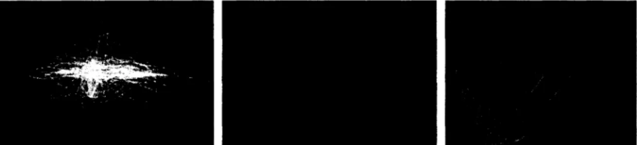
Figure 5: Sampled IRF time-steps colored by impulse palette index (2D projection of (qu)i..3 coordinates shown):
(Left) dinosaur with 5 impulse types; (Middle) plant with left (blue) and right (red) impulses; (Right) cloth with various door speeds: — UJQ (red), at rest (blue), and -h<^o (green).
3.5 Impulsively Sampling the Phase Portrait
By forcing the model with the impulse palette, IRFs can be impulsively sampled in the phase portrait. We use a simple random IRF sampling strategy pregenerated at the start of precomputation. A random sequence of impulse palette interactions are constructed, with each IRF integrated for a random duration, T € (Tmin, Tmax), bounded by time
scales of interest.
There are a couple of constraints on this process. First, the random sequence of impulse palette entries is chosen to be "representative of runtime usage" so that nonphysical or unused sequences do not occur. For example, the plant-in-pot example only models three pot motion speeds, {-^o, 0, +^o}> and therefore it is not useful to apply more than two same-signed ±vo velocity discontinuities in a row. Similarly, the cloth's door only changes angular velocity by \uo\ amounts, so that transitions from —c^o to -\-UJO are not sampled.
Second, a key point is that we sample enough IRFs of sufficiently long temporal duration to permit natural runtime usage. This is controlled using Tm^n and Tmax. In particular, dynamics can either (a) be played to completion (if
necessary), so that the model can naturally come to rest, or (b) expect to be interrupted based on physical modeling assumptions. As an example of the latter, the cloth's door has a 90 degree range of motion, so that IRFs associated with a nonzero angular velocity, u;, need be at most only 90/|u;| seconds in duration.
In order to produce representative clips of motion, we filter sampled IRFs to discard the shortest ones. These short orbits are not a loss, since they are used to span the phase portrait. We also prune orbits that end too far away from the start of neighbouring IRFs, and are "dead ends." We can optionally extend sampled orbits during precomputation, e.g., if insufficient data exists. Orbits terminating close enough (in the phase space distance metric) to be smoothly blended to other orbits, e.g., using Hermite interpolation, can be extended. In more difficult cases where the dynamics are very irregular, such as for the cloth, one can resort to local interpolation, e.g., /c-nearest neighbor, to extend orbits, but there are no quality guarantees. In general, we advocate sampling longer IRFs when possible.
While our sampling strategies are preplanned for use with standard offline solvers (see Figure 7), an online sam-pling strategy could be used. This would allow IRF durations, T, and new samsam-pling locations to be determined at runtime, and could increase sampling quality.
4 Reduced Global Illumination Model
A significant benefit of precomputing parameterizations of the deformable scene is that complex data-driven appear-ance models can then also be precomputed for real-time use. This parameterized appearappear-ance model corresponds to the second part of our phase space model (Equation 2). Once the reduced dynamical system has been constructed, we pre-compute an appearance model based on a low-rank approximation to the diffuse radiance transfer global illumination model for low-frequency lighting [SKS02]. Unlike hard stenciled shadows, the diffuse low-frequency lighting model produces "blurry" lighting and is more amenable to statistical modeling of deformation effects.
4.1 Radiance Transfer for Low-frequency Lighting
Following [SKS02], for a given deformed geometry, for each vertex point, p, we compute the diffuse interreflected transfer vector (Mp)i, whose inner product with the incident lighting vector, (Lp)i, is the scalar exit radiance at p, or
Lp = X ^= 1( M p ) i ( £P) i - Here both the transfer and lighting vectors are represented in spherical harmonic bases. For
a given reduced displacement model shape3, qu, we compute the diffuse transfer field M = M(qu) = (MPk)k=i..s
defined at s scene surface points, pk, k = l..s. Here MPfc is a 3n2 vector for an order-n SH expansion and 3 color
components, so that M is a large 3sn2 vector. We use n — 4 in all our examples, so that M has length 48s, i.e., 48 floats
per-vertex. Note that not all scene points are necessarily deformable, e.g., door, and some may belong to double-sided surfaces, e.g., cloth.
4.2 Dimensional Model Reduction
While we could laboriously precompute and store radiance transfer fields for all phase portrait state nodes, significant redundancy exists between them. Therefore, we also use least-squares dimensional model reduction to generate low-rank transfer field approximations. We note that, unlike displacement fields for which modal analysis suggests that least-squares projections can be optimal, there is no such motivation for radiance transfer.
Given Na deformed scenes with deformation coordinates ( q * , . . . , q ^a) , we compute corresponding scene transfer
fields, M*7' = M(q£), and their mean, M. We substract the mean from each transfer field, W; = W — M, and formally
assemble them as columns of a huge 3sn2-by-iVa zero-mean4 transfer data matrix,
(13)
We compute the SVD of Aa to determine the reduced low-rank transfer model, and so discover the reduced transfer
field coordinates q{ = qa( q j ) , j = 1... Na, for the Na deformed scenes. We denote the final rank-ra factorization 3The appearance model depends on the deformed shape of the scene (qu) but not its velocity (qu).
4Formally, there is no need to subtract the data mean prior to SVD (unlike for PCA where the covariance matrix must be constructed), but we do so because the first coordinate captures negligible variability otherwise.
as Aa « UaQa where Ua are the orthonormal transfer field basis vectors, and Qa = [q* • • - q ^a] are the reduced
appearance coordinates.
4.3 Interpolating Sparsely Sampled Appearances
Computing radiance transfer for all state nodes can be very costly and also perceptually unnecessary. We therefore interpolate the reduced radiance transfer fields across the phase portrait. Normalized Radial Basis Functions (NRBFs) are a natural choice for interpolating high-dimensional scattered data [NelOO]. We use K-means clustering [NelOO] to cluster phase portrait states into Na<^N clusters (see Figure 6). A representative state q£ closest to the kth cluster's
mean is used to compute radiance transfer (using the original state node's unreduced mesh to avoid compression artifacts in the lighting model). Model reduction is then performed on the radiance transfer fields for the 7Va states. In
the end, we know the reduced radiance values q£ at 7Va state nodes, i.e., q£ = qa(q£), k = 1... Na. These sparse
samples are then interpolated using a regularized NRBF approach (see Appendix B). This completes the definition of the deterministic state space model originally referred to in Equation 2.
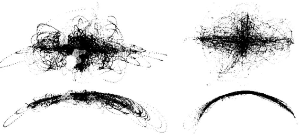
Figure 6: Clustering of deformed dinosaur scenes for transfer computation: (Left) Clustered shape coordinates {qu}
(Right) interpolated appearance coordinates { qa} . Only the first three (2D-projected) components of q are displayed.
5 Runtime Synthesis
At any runtime instant, we either "play an IRF" or are at rest, e.g., at the end of an IRF. Once an impulse is specified by an index from the impulse palette, we switch to a nearby IRF of that type and continue until either interrupted by another impulse signal or we reach the end of the IRF and come to rest. At each time-step we trivially lookup/compute qu and qa and use them to evaluate matrix-vector products for the displacement u = Uuqu and radiance transfer
M = Uaqa fields needed for graphical rendering. This approach has the benefits of being both simple and robust.
5.1 Approximating Impulse Responses
Given the problems associated with orbit interpolation (§3.1), we wish to transition directly between IRFs during simulation. To avoid transition (popping) artifacts, we smoothly transition between the state and the new IRF. We approximate the IRF at x' with the IRF £*(#, a7, aF) from a nearby state x by adding an exponentially decaying state
offset (x' — x) to the state,
^(x', a7, aF; T) « f *(*, a7, aF; T) + (xf - x)e~x\ (14)
where t = 0 , 1 , . . . , T, and A > 0 determines the duration of the offset decay. This approximation converges as x' —>#, e.g., as V is sampled more densely, but its chief benefit is that it can produce plausible motion even in undersampled cases (as in Figure 2). For rendering, appearance coordinates associated with £*(x, a1, aF; T) are also averaged,
Finally, the cost of computing the approximate shape and appearance coordinates is proportional to the dimension of the reduced coordinate vectors, 2ru 4- ra, and is cheap in practice.
5.2 Caching Approximate IRF References
A benefit of using a finite impulse palette To is that each state in the phase portrait can cache the D references to the nearest corresponding IRFs. Then at runtime, for the system in (or near) a given phase portrait state, x, the response to any of the D impulse palette excitations can be easily resolved using table lookup and IRF blending. By caching these local references at state nodes it is in principle possible to verify during precomputation that blending approximations are reasonable, and, e.g., don't lead to self-intersections.
5.3 Low-rank Model Evaluation
The two matrix-vector products, u = Uuqu and M — £/aqa, can be evaluated in software or in hardware. Our hardware
implementation is similar to [JP02a, SKS02] in that we compute the per-vertex linear superposition of displacements and transfer data in vertex programs. Given the current per-vertex attribute memory limitations of vertex programs (64 floats), some superpositions must be computed in software for larger ranks. Similar to [SKS02], we can reduce transfer data requirements (by a factor of n2 = 16) by computing and caching the 3ra per-vertex light vector inner-products in
software, i.e., fixing the light vector. Each vertex's color linear superposition then involves only ra 3-vectors.
Scene Dinosaur Cloth Plant Deformable Model F 49376 6365 6304 V 24690 3310 3750 DOF 74070 9930 11250 ru 12 30 18 relErr 0.5% 1.5% 2.0% Appearance Model F 52742 25742 11184
v
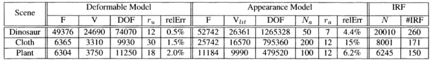
Kt 26361 16570 9990 DOF 1265328 795360 479520 Na 50 200 100 ra 1 12 12 relErr 4.4% 15% 6.2% IRF N 20010 8001 6245 #IRF 260 171 150 Table 1: Model Statistics: The ru and ra ranks correspond to those used for frame rate timings in Table 2.6 Results
We applied our method to three deformable scenes typical of computer graphics that demonstrate some strengths and weaknesses of our approach. Dynamics and transfer precomputation and rendering times are given in Table 2, and model statistics are in Table 1. The dynamics of each of the three models were precomputed over the period of a day or more using standard software (see Figure 7). Radiance transfer computations took on the order of a day or more due to polygon counts, and sampling densities, Na.
Scene Dinosaur Cloth Plant 1 Precomputation
1 Dynamics
33h21m 16h46m « 1 weekTransfer 74h 71h27m l l h 4 0 m
Frame rates (in SW) Defo
173 350 472
Defo + Trnsfr 82 (175 in HW)
149 200
Table 2: Model timings on an Intel Xeon 2.0GHz, 2GB-266MHz DDR RDRAM, with GeForce FX 5800 Ultra. Run-time matrix-vector multiplies computed in software (SW) using an Intel performance library, except for the dinosaur example that fits into vertex program hardware (HW).
The cloth example demonstrates interesting soft shadows and illumination effects, as well as subtle nonlinear deformations typical of cloth attached to a door (see Figure 8). This is a challenging model for data-driven deformation because the material is thin, and in persistent contact, so that small deformation errors can result in noticeable self-intersection. By increasing the rank of the deformation model (to ru = 30), the real-time simulation avoids visible
intersection5. Unlike the other examples, the complex appearance model appears to have been undersampled by 5Using a larger cloth "thickness" during precomputation would also reduce intersection artifacts.
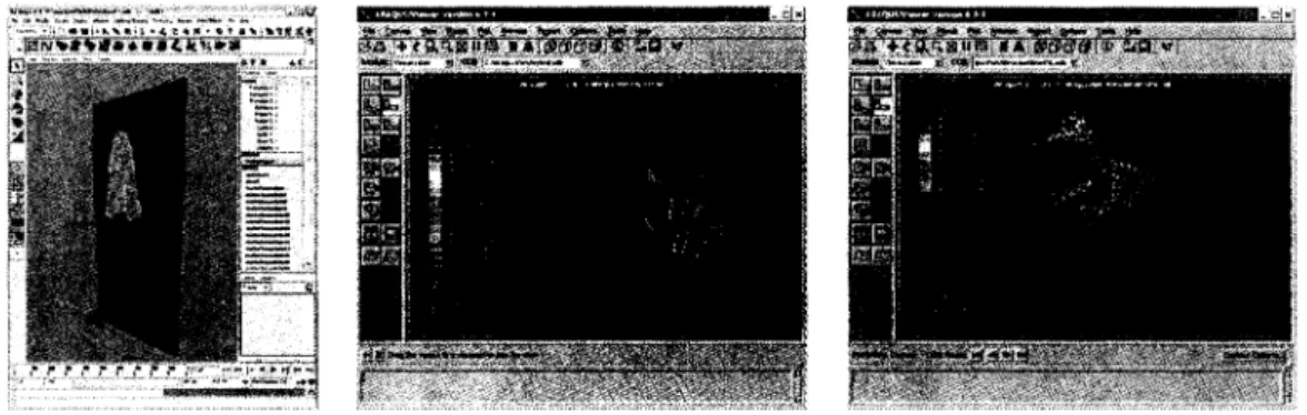
Figure 7: Precomputing real-time models with offline simulators: (Left) cloth precomputed in Alias|Wavefront Maya; (Middle,Right) models precomputed by an engineering analysis package (ABAQUS) using an implicit Newmark inte-grator.
the cluster shape sampling (7Va = 200) since there is some uneveness in interpolated lighting and certain cloth-door
shadows lack proper variation.
Figure 8: Dynamic cloth states induced by door motions: (Left) cloth and door at rest; (Right) cloth pushed against moving door by air drag.
The plant example has interesting shadows and changing visibility, and the dynamics involve significant multi-leaf collisions (see Figures 10, 11 and 12). The plant was modeled with 788 quadrilateral shell finite elements in ABAQUS, with the many collisions accurately resolved with barrier forces and an implicit Newmark integrator.
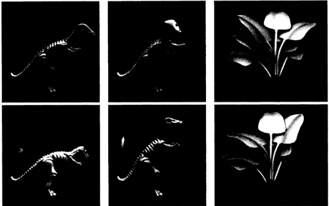
The rubber dinosaur had the simplest dynamics of the three models, and did not involve collisions. It was precom-puted using an implicit Newmark integrator with 6499 FEM tetrahedral elements, and displacements were interpolated onto a finer displaced subdivision surface mesh [LMH00]. However, the radiance transfer data model was easily the largest of the three, and includes interesting self-shadowing (on the dinosaur's spines) and color bleeding (see Fig-ure 11). Runtime simulation images, and some reduced basis vectors, or modes, of the dinosaur's displacement and radiance transfer models are shown in Figure 14.
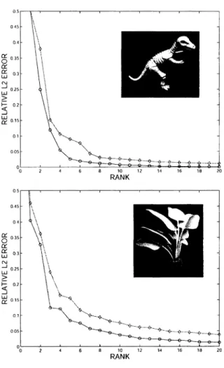
All examples display interesting dynamics and global illumination behaviors. Significant reductions in the rank of the displacement and appearance models were observed, with only a modest number of flops per vertex required to synthesize each deformed and illuminated shape. In particular, Figure 13 shows that the singular values converge quickly, so that useful approximations are possible at low ranks. In general, for a given error tolerance, appearance models are more complex than deformation models. However, when collisions are present, low-rank deformation approximations can result in visible intersection artifacts so that somewhat higher accuracy is needed.
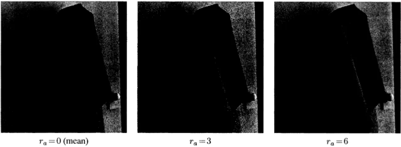
ra — 0 (mean)
Figure 9: Reduced radiance transfer illuminations for an arbitrary cloth pose illustrate improving approximations as the rank ra is increased.
Figure 10: View of plant from behind
7 Summary and Discussion
Our method permits interactive models of physically based deformable scenes to be almost entirely precomputed using data-driven tabulation of state space models for shape and appearance. Using efficient low-rank approximations for the deformation and appearance models, extremely fast rendering rates can be achieved for interesting models. Such approaches can assist traditional simulation in applications with constrained computing resources.
Future work includes improving dynamics data quality by using better non-random sampling strategies for IRFs. Building better representations for temporal and spatial data could be investigated using multiresolution and "best basis" statistics. Generalizing the possible interactions, e.g., for contact, and supporting more complex scenes remain important problems. Extensions to deformable radiance transfer for nondiffuse models, and importance-based sparse shape sampling are also interesting research areas.
Acknowledgments: We would like to acknowledge the helpful criticisms of several anonymous reviewers,
assis-tance from Christopher Twigg and Matthew Trentacoste, hardware from NVIDIA, Cyberware for the dinosaur model, and the Carnegie Mellon Graphics group.
Figure 11: Interactive dynamic behaviors resulting from applied impulses
Figure 12: Dynamic interpolated shadows
A Output-Sensitive SVD
Computing the Singular Value Decomposition (SVD) of a huge m-by-n matrix is very costly ((9 (ran min (m,n))
[GL96]), and is wasteful for low-rank matrices, especially when only leading singular factors are desired. Fortunately
fast out-of-core algorithms exist, and we use the following simple direct method to approximate the largest orthogonal
singular factors for a large approximately low-rank m-by-n matrix, A. We begin by computing a drop tolerance rank-r
unmodified Graham-Schmidt orthogonal factorization, A « EX, for a given sufficiently small tolerance e € (0,1),
where E is an m-by-r orthogonal Graham basis matrix, and X is an r-by-n matrix of expansion coefficients. The
factorization proceeds by processing one column of A at a time, so that the matrix A is never explicitly constructed.
For a given column, A
:j, and current rank of the Graham basis, r, the basis is expanded only if the relative residual
RANK
Figure 13: Model reduction: Relative I2 error versus
model rank, r
uand r
a, for the displacement (blue) and
radiance transfer (red) models.
error is greater than the (drop tolerance) threshold, e
9i.e.,
\\A
:j-A
:3\\>s\\A
:Jl
(16)
where A
:j is the projection of A
:j into the current rank-f Graham basis. The final low-rank SVD is then found by
taking the SVD of X = USV
Tand multiplying as follows:
A w EX = E{USV
T) = (EU)SV
T= USV
1 (17)In practice we discard all factors whose singular values when normalized by the largest value are less than some
desired accuracy (> e). We refer the interested reader to [GL96, BraO2, SZOO] for related algorithms.
B NRBF Appearance Interpolation
Normalized radial basis functions (NRBFs) are used to interpolate q
a(q
n) at all phase portrait q
u. We center radial
basis functions at all of the M
atransfer sampled state nodes,
(18)
(19)
q£ - q j | | / a
2) , k = 1 . . . M
a,
where a is the radial scale of the basis functions. The NRBF interpolant is
transfer mode 3 transfer mode 5 transfer mode 6 Figure 14: Dinosaur modes: (Top) displacement mode shapes; (Bottom) radiance transfer modes.
where c£ are the unknown coefficients, and (j>k(qu) are normalized basis functions,
(20)
The components of c£ can be determined by substituting the data, q£ = qa(q*). k = 1 . . . Ma, to obtain
(21)
To avoid ill-conditioning which occurs as Ma or a increase, i.e., over-fitting, the NRBF equation is solved using
truncated SVD.
References
[AM00] Marc Alexa and Wolfgang Miiller. Representing Animations by Principal Components. Computer Graph-ics Forum, 19(3):411^18, August 2000.
[AMS97] C.G. Atkeson, A.W. Moore, and S. Schaal. Locally Weighted Learning for Control. AI Review, 11:75-113, 1997.
[AS92] Ralph H. Abraham and Christopher D. Shaw. Dynamics - the Geometry of Behavior. Addi son-Wesley, 1992.
[BFA02] Robert Bridson, Ronald P. Fedkiw, and John Anderson. Robust Treatment of Collisions, Contact, and Friction for Cloth Animation. ACM Transactions on Graphics, 21(3):594-603, July 2002.
[BraO2] Matthew E. Brand. Incremental Singular Value Decomposition of Uncertain Data with Missing Values. In Proc. of Euro. Conf on Comp. Vision (ECCV), volume 2350, pages 707-720, May 2002.
[BV99]
[BW98]
[CDA99]
[CGC+02]
Volker Blanz and Thomas Vetter. A Morphable Model for the Synthesis of 3D Faces. In Proc. of
S1GGRAPH 99, pages 187-194, August 1999.
David Baraff and Andrew P. Witkin. Large Steps in Cloth Simulation. In Proceedings ofSlGGRAPH 98,
pages 43-54, July 1998.
S. Cotin, H. Delingette, and N. Ayache. Realtime Elastic Deformations of Soft Tissues for Surgery
Simulation. IEEE Trans, on Vis. and Comp. Graphics, 5(l):62-73, 1999.
Steve Capell, Seth Green, Brian Curless, Tom Duchamp, and Zoran Popovic. A Multiresolution
Frame-work for Dynamic Deformations. In ACM S1GGRAPH Symposium on Computer Animation, pages 4 1 ^ 8 ,
July 2002.
[DDCB01] Gilles Debunne, Mathieu Desbrun, Marie-Paule Cani, and Alan H. Barr. Dynamic Real-Time
Defor-mations Using Space & Time Adaptive Sampling. In Proceedings of SIGGRAPH 200J, pages 31-36,
August 2001.
[EK02] Cass Everitt and Mark J. Kilgard. Practical and Robust Stenciled Shadow Volumes for
Hardware-Accelerated Rendering. Technical report, NVIDIA Corporation, Inc., Austin, Texas, 2002.
[GH83] John Guckenheimer and Philip Holmes. Nonlinear oscillations, dynamical systems, and bifurcations of
vector fields (AppL math, set; v. 42). Springer-Verlag New York, Inc., 1983.
[GKS02] Eitan Grinspun, Petr Krysl, and Peter Schroder. CHARMS: A Simple Framework for Adaptive
Simula-tion. ACM Transactions on Graphics, 21 (3):281-290, July 2002.
[GL96] Gene H. Golub and Charles F. Van Loan. Matrix Computations. Johns Hopkins University Press,
Balti-more, third edition, 1996.
[GTH98] Radek Grzeszczuk, Demetri Terzopoulos, and Geoffrey Hinton. NeuroAnimator: Fast Neural Network
Emulation and Control of Physics-Based Models. In Proceedings of SIGGRAPH 98, pages 9-20, July
1998.
[HeiOl] Wolfgang Heidrich. Interactive Display of Global Illumination Solutions for Non-diffuse Environments
- A Survey. Computer Graphics Forum, 20(4):225-244, 2001.
[JP99] Doug L. James and Dinesh K. Pai.
ARTDEFO- Accurate Real Time Deformable Objects. In Proc. of
SIGGRAPH 99, pages 65-72, August 1999.
[JP02a] Doug L. James and Dinesh K. Pai. DyRT: Dynamic Response Textures for Real Time Deformation
Simulation With Graphics Hardware. ACM Trans, on Graphics, 21(3):582-585, July 2002.
[JP02b] Doug L. James and Dinesh K. Pai. Real Time Simulation of Multizone Elastokinematic Models. In
Proceedings of the IEEE International Conference on Robotics and Automation, pages 927-932,
Wash-ington, DC, 2002.
[JP03] Doug L. James and Dinesh K. Pai. Multiresolution Green's Function Methods for Interactive Simulation
of Large-scale Elastostatic Objects. ACM Trans, on Graphics, 22(l):47-82, 2003.
[KGP02] Lucas Kovar, Michael Gleicher, and Frederic Pighin. Motion Graphs. ACM Transactions on Graphics,
21(3):473-482, July 2002.
[KJP02] Paul G. Kry, Doug L. James, and Dinesh K. Pai. EigenSkin: Real Time Large Deformation Character
Skinning in Hardware. In SIGGRAPH Symposium on Computer Animation, pages 153-160, July 2002.
[KLM01] P. Krysl, S. Lall, and J. E. Marsden. Dimensional model reduction in non-linear finite element dynamics
of solids and structures. International Journal for Numerical Methods in Engineering, 51:479-504, 2001.
[LCR+02] Jehee Lee, Jinxiang Chai, Paul S. A. Reitsma, Jessica K. Hodgins, and Nancy S. Pollard. Interactive
Control of Avatars Animated With Human Motion Data. ACM Transactions on Graphics,
21(3):491-500, July 2002.
[Len99] Jerome Edward Lengyel. Compression of Time-Dependent Geometry. In ACM Symposium on Interactive 3D Graphics, pages 89-96, April 1999.
[LJM01] Erik Lindholm, Mark J.Kilgard, and Henry Moreton. A User-Programmable Vertex Engine. In Proceed-ings ofSIGGRAPH 2001, pages 149-158, Aug 2001.
[LMH00] A. Lee, H. Moreton, and H. Hoppe. Displaced Subdivision Surfaces. In Proc. ofSIGGRAPH 2000, pages 85-94, 2000.
[Lum67] J. L. Lumley. The structure of inhomogeneous turbulence. In Atmospheric turbulence and wave propa-gation, pages 166-178, 1967.
[NelOO] Oliver Nelles. Nonlinear System Identification: From Classical Approaches to Neural Networks and Fuzzy Models. Springer Verlag, December 2000.
[OH99] J.E O'Brien and J.K. Hodgins. Graphical Modeling and Animation of Brittle Fracture. In SIGGRAPH 99 Conference Proceedings, pages 111-120, 1999.
[OHHM02] Marc Olano, John C. Hart, Wolfgang Heidrich, and Michael McCool. Real-Time Shading. A.K.Peters, 2002.
[PBMH02] Timothy J. Purcell, Ian Buck, William R. Mark, and Pat Hanrahan. Ray Tracing on Programmable Graphics Hardware. ACM Transactions on Graphics, 21(3):703-712, July 2002.
[PMTH01] Kekoa Proudfoot, William R. Mark, Svetoslav Tzvetkov, and Pat Hanrahan. A Real-Time Procedural Shading System for Programmable Graphics Hardware. In Proceedings of SIGGRAPH 2001, pages 159-170,2001.
[POAU00] Mark S. Peercy, Marc Olano, John Airey, and P. Jeffrey Ungar. Interactive Multi-Pass Programmable Shading. In Proceedings of SIGGRAPH 2000, pages 4 2 5 ^ 3 2 , 2000.
[Poi57] H. Poincare. Les Methodes Nouvelles de la Mecanique Celeste /, //, ///. (Reprint by) Dover Publications, 1957.
[PW89] A. Pentland and J. Williams. Good Vibrations: Modal Dynamics for Graphics and Animation. In Com-puter Graphics (SIGGRAPH 89), volume 23, pages 215-222, 1989.
[RP01] L. M. Reissell and Dinesh K. Pai. Modeling Stochastic Dynamical Systems for Interactive Simulation. Computer Graphics Forum, 20(3):339-348, 2001.
[Sha90] A.A. Shabana. Theory of Vibration, Volume II: Discrete and Continuous Systems. Springer-Verlag, New York, NY, first edition, 1990.
[SIC01] Peter-Pike J. Sloan, Charles F. Rose III, and Michael F. Cohen. Shape by Example. In ACM Symp. on Interactive 3D Graphics, pages 135-144, March 2001.
[SKS02] Peter-Pike Sloan, Jan Kautz, and John Snyder. Precomputed Radiance Transfer for Real-Time Rendering in Dynamic, Low-Frequency Lighting Environments. ACM Transactions on Graphics, 21(3):527-536, July 2002.
[SSSEOO] Arno Schodl, Richard Szeliski, David H. Salesin, and Irfan Essa. Video Textures. In Proc. ofSIGGRAPH 2000, pages 489-498, July 2000.
[Sta97] J. Stam. Stochastic Dynamics: Simulating the Effects of Turbulence on Flexible Structures. Computer Graphics Forum, 16(3), 1997.
[SZOO] Horst D. Simon and Hongyuan Zha. Low-Rank Matrix Approximation Using the Lanczos Bidiagonal-ization Process with Applications. SI AM Journal on Scientific Computing, 21(6):2257-2274, 2000. [TPBF87] Demetri Terzopoulos, John Platt, Alan Barr, and Kurt Fleischer. Elastically Deformable Models. In
Computer Graphics (Proceedings of SIGGRAPH 87), volume 21(4), pages 205-214, July 1987.
[Wei86] Jerry Weil. The Synthesis of Cloth Objects. In Computer Graphics (Proceedings of S1GGRAPH 86), volume 20(4), pages 49-54, August 1986.