Sharif University of Technology
Scientia IranicaTransactions E: Industrial Engineering http://scientiairanica.sharif.edu
Copula Gaussian graphical modeling of biological
networks and Bayesian inference of model parameters
H. Farnoudkia and V. Purutcuoglu
Department of Statistics, Middle East Technical University, Ankara, Turkey.
Received 25 August 2017; received in revised form 12 April 2018; accepted 20 May 2019
KEYWORDS Copula Gaussian graphical model; Reversible jump Markov chain Monte Carlo algorithm; Biological networks; F-measure;
Systems biology.
Abstract. A proper understanding of complex biological networks facilitates a better perception of those diseases that plague systems and ecient production of drug targets, which is one of the major research questions under the personalized medicine. However, the description of these complexities is challenging due to the associated continuous, high-dimensional, correlated and very sparse data. The Copula Gaussian Graphical Model (CGGM), which is based on the representation of the multivariate normal distribution via marginal and copula terms, is one of the successful modeling approaches to presenting such types of problematic datasets. This study shows its novelty by using CGGM in modeling the steady-state activation of biological networks and making inference of the model parameters under the Bayesian setting. In this regard, the Reversible Jump Markov Chain Monte Carlo (RJMCMC) algorithm is suggested in order to estimate the plausible interactions (conditional dependence) between the systems' elements, which are proteins or genes. Furthermore, the open-source R codes of RJMCMC are generated for CGGM in dierent dimensional networks. In this regard, real datasets are applied, and the accuracy of estimates via F-measure is evaluated. From the results, it is observed that CGGM with RJMCMC is successful in presenting real and complex systems with higher accuracy. © 2019 Sharif University of Technology. All rights reserved.
1. Introduction
In recent years, the term network or system has become one of the most popular concepts in various sciences, ranging from computer engineering to biology. Although its property varies in all these disciplines, which is why it is implemented by means of distinct assumptions, it should be noted that a common struc-ture constructs a mechanism specialized for one or more functions. In terms of biology, a network represents a set of reactions that describes a particular process
*. Corresponding author.
E-mail addresses: [email protected] (H. Farnoudkia); [email protected] (V. Purutcuoglu) doi: 10.24200/sci.2019.5071.1076
of a species by means of genomic particles, denoting genes or proteins and their interactions. Thereby, understanding such complexity and describing it math-ematically can open new avenues for researchers for both understanding various diseases and producing appropriate treatment under personalized medicine.
Therefore, graphical modeling is one of the very common tools to represent any dimensional network where each variable is shown by a node, and the relationship between two nodes is presented by an undi-rected edge. The Gaussian Graphical Model (GGM) is the probabilistic version of the graphical approach, where nodes, also called states, are described by a multivariate normal distribution with a p-dimensional mean vector = (1; 2; : : : ; p) and a (p
p)-dimensional covariance matrix for totally p nodes [1]. The precision matrix, which is the inverse of , also
denoted by = 1, is an expression that represents
the conditional dependence between nodes, such that the signicantly large values show highly possible dependency between the two related nodes, given the remaining nodes in the network. In this respect, the mathematical description of the model is shown below: Yp= Y p+ "; (1)
where Ypstands for the state of the pth node, and Y p
shows the states of all other nodes except the pth node, respectively. is the vector of the regression coecient associated with Y p, " shows p-dimensional vector for
the random error. Accordingly, the distribution of Y is shown as follows:
f (Yj; ) = (2) n2 det () 12
expf 12(Y )T 1(Y ) g: (2)
Herein, det(:) and (:)T represent the determinant
and the transpose of the given matrix, respectively. Thus, in the inference of this model, has a direct relation with via = pp=pp in which pp is
the ((p 1) p)-dimensional submatrix of when the associated term of the pth node is discarded. Thus, the knowledge of implies the knowledge of , resulting in the information about the conditional dependency between the related nodes. In the estimation of , dierent methods can be applied. Among many alternatives, Friedman et al. (2008) [2] considered the graphical lasso, also known as glasso, approach by infer-ring the entries of via the penalized likelihood method whose penalty constant controls via l1-norm. On
the other hand, Meinshausen and Buhlmann (2006) [3] suggested the neighborhood selection method, which is fully nonparametric and is based on the threshold gradient descent algorithm for the estimation of . However, the major challenge of all these algorithms is the computational limitation in the inference of realistically high-dimensional systems.
This study aims to implement the Bayesian frame-work as an alternative to the underlying frequentist and non-parametric approaches. The suggested method is implemented in the form of the combination of GGM and the Gaussian copula [4], resulting in the copula GGM model. The main advantage of this model is that it can overcome the modeling problem of high-dimensional systems by describing the complex GGM model and its multivariate normal density via pieces of marginal and copula terms within the copula GGM representation. CGGM has been already proposed in the study of Dobra and Lenkoski (2011) [5] to describe the functional disability data. In that work, the inference is conducted via the Reversible Jump Markov Chain Monte Carlo method (RJMCMC). Here,
the novelty of this study lies in adopting this approach to construct the structure of a biological network and infer its model parameters. Furthermore, as the second novelty, this study writes the functional codes via the R programming language so that the codes can be appli-cable to all biological networks under the steady-state condition and distinct dimensions, i.e., the number of nodes or proteins. Of note, the codes are available upon request. Accordingly, to compare the performance of our algorithm with others, three datasets have been used. Initially, the social survey dataset of Dobra and Lenkoski (2011) [5], which is also applied as a benchmark dataset in comparative analyses, has been implemented [6,7]. Then, an actual biological network, called cell signaling network, is used, and the results are interpreted. Lastly, an ovarian cancer dataset, whose true interactions can be biologically validated from the literature, should be implemented. Finally, our ndings are compared with the outputs of Mohammadi (2015) [6], where the inference is performed via the birth-and-death algorithm in place of RJMCMC for the same CGGM.
Hence, in the process of organizing this study, the Gaussian graphical model and copulas are introduced in Section 2. In Section 3, the method of inference is introduced in detail. Then, in Section 4, the suggested methods are applied to dierent datasets. Lastly, our ndings are summarized, and some suggestions for the future works are made in Section 5.
2. Materials and methods
In this part, initially, the general idea of graphical networks, which is one of the common ways to show the relationship between factors in a mathematical model, is explained. Based on the statistical analysis of biological networks, when the number of genes or other kinds of variables is large and their correlation matrix is sparse, the application of a graphical version of the network may boost readers' imagination about the structure of genes or variables. In this representation, the Gaussian copula graphical model is performed as it enables one to partition a high-dimensional joint dis-tribution function as pieces of marginal that are bound by a separate copula term when the data are described by multivariate normal distribution. By means of normality, we can also simplify the correlation between variables due to the property of the conditional inde-pendency. Finally, by using the RJMCMC algorithm in the inference of the network, we can benet from the exibility of the Bayesian method when the data are limited and the dimension of the network is large.
Hence, in the following parts, the mathematical details of the graphical model, the Gaussian graphical model, the Gaussian copula approach, and the selected Bayesian algorithm are presented in order.
2.1. Graphical model
Let a data matrix Y with p variables and n samples be presented; herein, an attempt is made to obtain the relationship between Yi and Yj for i 6= j given the
remaining variables. In this type of networks, which is common in social surveys and biological aspects, each variable is shown by a node in a graph and the conditional dependence between two nodes is presented by an undirected edge. Hereby, if E denotes the set of available edges under an undirected structure, (i; j) 2 E equals (j; i) 2 E, showing that Yi and Yj
are conditionally dependent (i; j = 1; 2; : : : ; p and also Yi?YjjYV ni;j for V = 1; 2; : : : ; p). This structure is
called the pairwise Markov property [1]. 2.1.1. Gaussian graphical model
Now, it is assumed here that vector Y follows a p-dimensional multivariate normal distribution via Np 0; 1. Here, is the inverse of the covariance
matrix, which is also called the precision matrix. Hence, for n samples, the likelihood function of Y can be written as follows:
Y1:nj/ jjn 2 exp
1 2tr
TU; (3)
where j:j and tr(:) describe the determinant and the trace of the given expression, respectively, and T is the transpose of the given matrix as used beforehand. Finally, U is the trace of the YTY matrix. Thus, a
graphical model with V nodes and E edges, (V; E), for Np 0; 1 is presented where V = (1; 2; :::; p) is
called the Gaussian Graphical Model (GGM). 2.2. Gaussian copula
If the normality assumption does not hold for the data matrix, the copula can solve the problem by combining data such that their joint distribution is Gaussian with the same covariance matrix [4,1,8]. For binary and ordinal categorical data, a continuous latent variable Z is introduced [5,6,9,10] by dening some increasing thresholds = (;0; ;1; : : : ; ;!). Therefore:
yj =
!
X
l=1
l 1;l 1<zj
;l; (4)
for j = 1; 2; :::; n. The relationship between Yijand Zij
satises the following constraint.
yij < yik! zij< zik; zij < zik! yij yik: (5)
Then, by dening the interaction of the correlation matrix in terms of as:
Yi;j() =
1 i;j
q ( 1)
i;i( 1)j;j
; (6)
and ZVNp 0; 1, a one-to-one correspondence with
observed data can be obtained as follows:
~
Zi= Zi=(i;i1)
1 2 and
Yi= F 1
Z~i
: (7)
In Eq. (6), i;iand j;j indicate the diagonal entries of
the ith and jth nodes, respectively. Accordingly, i;jis
the precision value between the ith and jth nodes. On the other hand, in Eq. (7), F 1 and stand for the
inverse of the cumulative distribution functions (cdf) and cdf of the normal distribution, respectively. Hence, by standing C(u1; : : : ; upjY ) as the Gaussian copula
with (p p)-dimensional correlation matrix for the p random sample from the standard uniform distribution, we have:
p (Y1< y1; : : : ; Yp< yp)
= C(F1(y1) ; : : : ; Fp(yp) jY ()):
This study decomposes the multivariate normal distri-bution of the states via the Gaussian copula model with the normal marginal distributions. This new probability distribution function is used to calculate the likelihood within the Bayesian framework. In doing so, GGM can be performed under any dimensional systems since the high-dimensional multivariate normal density can be partitioned via the copula term. 2.3. Reversible jump Markov chain Monte
Carlo method
The Reversible Jump Markov Chain Monte Carlo method (RJMCMC) is an approach that mostly deals with the Cholesky decomposition to obtain a positive denite precision matrix due to its conjugate advan-tages in prior distribution for the precision matrix, which is considered as the G-Wishart distribution [11] with a density:
p (jG)=I 1
G(; D)det
22 exp 1 2tr
TD: (8) In this expression, G implies the given graphical structure of the data. On the other hand, the G-Wishart prior is a generalized version of the chi-square distribution and the conjugate with the multivariate normal density. The sampling algorithm from the G-Wishart distribution was performed by Lenkoski (2013) [12]. Thus, the posterior distribution, , of the given G is presented as the G-Wishart distribution with parameters + n and D + U. In this expression, > 2, D = Ipis the p-dimensional identity matrix and
U = Pn
j=1yjy T
j, i.e., the trace of YTY, as dened
be-forehand. In Eq. (8), the normalizing constant IG(; D)
is not always easy to obtain [13]. When G is not a complete graph and is non-decomposable, this constant is calculated by a Monte Carlo method. Accordingly,
a double reversible jump algorithm was introduced by Lenkoski (2013) [12] to obtain the normalizing constant of the G-Wishart distribution.
Further, the Cholesky decomposition partitions the matrix into a lower triangle matrix and its trans-pose in a way that = 'T' denotes a chi-square
distribution into the square of the standard normal distribution. Here, ' is the upper triangle matrix, in which zero implies no relationship between the two corresponding elements. Finally, under the normality of data, two strictly positive precision parameters p=
g = 0:1 and RJMCMC are repeated in the following
steps until convergence is achieved [4]. 2.3.1. Resampling the latent data
In the rst stage of the RJMCMC algorithm, the latent variable Z is used instead of Y if Y's are not normal [5,3]. Here, Z is an (n p)-dimensional matrix and, for each column, which is related to each node, we calculate its minimum L and its maximum U as the vectors of p elements.
In this step, by using matrix and vectors L and U, other Zi's are generated from truncated normal in
the Li and Ui distributions in the following form:
ZijZini N i; 2i
; (9)
where: i=
X
y2bd(i)
i;y
i;izy;j;
for:
bd (i) = fy 2 (1; : : : ; p) : (i; j) 2 Eg ; when:
E = f(i; j) ji;y 6= 0; i 6= yg; 2i = 1 i;i;
and: i;i= 1
i;i:
In the second step, these zi;j's will be used.
2.3.2. Resampling the Precision Matrix
In this step, matrix is calculated by using the latent variables from the previous stage, and the Cholesky decomposition of matrix is applied. For non-zero diagonal elements, a Metropolis-Hasting update [2] of ' is done by sampling a value from a normal distribution truncated below at zero with a mean 'i;i
and a variance 2
p. Then, is replaced by the related
diagonal elements of ' and ' and transformed to '0
with a probability minfRp; 1g, where:
Rp=
'i;i
p
p
('
i;i)
+n+nb(i) 1R0
p; (10)
denoting that:
R0p= expf 12tr(0 )T D + tr ZTZg: (11)
In addition, the candidate value 0 = '0T'0results in
= 'T'.
For non-diagonal elements of ', a new is sam-pled from N(i; g2). In these cases, ' is transformed
to '0 with a probability minfR0 p; 1g.
2.3.3. Resampling the graph
In the third step, only one element of the Cholesky matrix 'i;j, which is obtained in the previous step, is
selected randomly. If there is no edge between Yi and
Yj, it will be changed by a value from N('i;j; 2g) in '
with a probability minfRp; 1g, where:
Rp=g
p
2'i;iIIG(; D) G0(; D)
expf 12tr( 0 )T D + tr ZTZ
+('0i;j 'i;j)
2
22
g g; (12)
Here, '0 stands for the proposal ' and G0is a graph in
which all elements coincide with G except Gi;j, which
is supposed to be the edge between related nodes. If there is an edge between Yi and Yj, it will be replaced
by zero in ' with a probability minfR0
p; 1g, where:
R0 p=(g
p
2'i;i) 1IIG(; D) G0(; D)
expf 1
2tr( 0 )T D + tr ZTZ
+('0i;j 'i;j)2 22
g g: (13)
In this stage, since the dimensionality of the parameter space changes by a one-unit increase or one-unit de-crease, the reversible jump Markov chain methodology is performed. Then, this graph in the rst step of the algorithm is used, and the process continues until convergence is reached.
3. Applications
In order to evaluate the RJMCMC method in terms of accuracy and assess its performance for the rst time in real biological systems, the code of the R programming language is originally generated with a function for each stage by deriving it from the sample precision matrix as the initial matrix after 200,000 iterations for three datasets. The rst case of data is the Rochdale dataset and is used to conduct comparative analysis of dierent inference methods [14]. The second data are the real data applied to construct the cell signaling
pathway, and the third data represent the combination of endometrial and ovarian carcinoma [15-17].
3.1. Rochdale data
The Rochdale data are binary (yes/no) data collected from 665 samples to assess the relationship among eight factors aecting the economic activities specic to women. These eight variables are named as follows: a (wife economically active), b (age of wife > 38), c (husband unemployed), d (child 4), e (wife's educa-tion at the high-school level or beyond), f (husband's education at the high-school level or beyond), g (Asian origin), and h (other household member working). In the case of analyses, it is claimed that there are at least two-way interaction eects whose minimal sucient statistics are the following pair of variables: ffg, ef, dh, dg, cg, cf, ce, bh, be, bd, ag, ae, ad, acg. Then, by including variable h, which changes as very fast and very slow as the two new random variables, the data are observed in Table 1. More details about this dataset can be also found in the studies of Whittaker (1990) [1] and Dobra and Lenkoski (2011) [5]. Hereby, from the inference of this dataset via RJMCMC, 15 edges are found: (a; c), (a; d), (a; e), (a; g), (b; d), (b; e), (b; h), (c; e), (c; f), (c; g), (d; g), (d; h), (e; f), (e; g), and (f; g). The 14 edges that represent the validated links from the study of Whittaker (1990) [1] are exactly the same as what have been obtained from the RJMCMC codes except (e; g) edge.
As a result, in these analyses, the data are initially transformed to Gaussian. Then, by applying our RJMCMC codes, the latent variables Z are resam-pled based on entries of the initial matrix, which is considered as the sample covariance matrix in our
study. Next, the precision matrix is resampled by taking the latent data produced in the rst step, and the graph is resampled by only one element, which is selected randomly from the Cholesky decomposition of the precision matrix in the second step. This process continues until convergence is reached. In this example, this process is iterated up to 1,000,000 times, of which the rst 200,000 runs are supposed to be in the burn-in period. The adjacency matrix is obtaburn-ined from the mean of the estimated entries of the precision matrix and, thereby, represents the estimated structure of the links, as shown in Table 2.
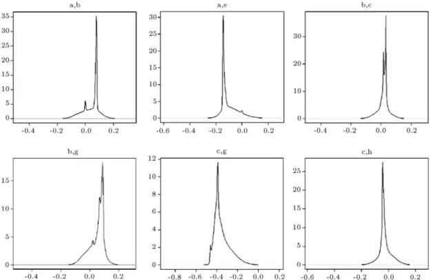
In this matrix, the entry 1 indicates the link between the pairs of variables, and the entry 0 implies no link between them. Further, Figure 1 presents some examples from the estimated density of selected pairs in the precision matrix after the burn-in period with 200,000 MCMC runs. In these plots, it is observed that each estimated density is unimodal, and the model parameters reach convergence.
Table 2. The adjacency matrix of the Rochdale data estimated by 1,000,000 RJMCMC iterations, where the rst 200,000 runs take place in the burn-in period.
a b c d e f g h
a 0 0 1 1 1 0 1 0
b 0 0 0 1 1 0 0 1
c 1 0 0 0 1 1 1 0
d 1 1 0 0 0 0 1 1
e 1 1 1 0 0 1 1 0
f 0 0 1 0 1 0 1 0
g 1 0 1 1 1 1 0 0
h 0 1 0 1 0 0 0 0
Table 1. The lexicographical ordered Rochdale data [7].
5 0 2 1 5 1 0 0 4 1 0 0 6 0 2 0
8 0 11 0 13 0 1 0 3 0 1 0 26 0 1 0
5 0 2 0 0 0 0 0 0 0 0 0 0 0 1 0
4 0 8 2 6 0 1 0 1 0 1 0 0 0 1 0
17 10 1 1 16 7 0 0 0 2 0 0 10 6 0 0
1 0 2 0 0 0 0 0 1 0 0 0 0 0 0 0
4 7 3 1 1 1 2 0 1 0 0 0 1 0 0 0
0 0 3 0 0 0 0 0 0 0 0 0 0 0 0 0
18 3 2 0 23 4 0 0 22 2 0 0 57 3 0 0
5 1 0 0 11 0 1 0 11 0 0 0 29 2 1 1
3 0 0 0 4 0 0 0 1 0 0 0 0 0 0 0
1 1 0 0 0 0 0 0 0 0 0 0 0 0 0 0
41 25 0 1 37 26 0 0 15 10 0 0 43 22 0 0
0 0 0 0 2 0 0 0 0 0 0 0 3 0 0 0
2 4 0 0 2 1 0 0 0 1 0 0 2 1 0 0
Figure 1. The density of some of the estimated entries in the precision matrix for the Rochdale data after the 1,000,000 MCMC iterations, where the rst 200,000 runs take place in the burn-in period.
Table 3. The adjacency matrix of the cell signaling pathway data estimated by the 1,000,000 iterations of the birth-and-death algorithm [23], where the rst 200,000 runs take place in the burn-in period.
a b c d e f g h
a 0 1 1 1 1 0 1 1
b 1 0 0 1 1 1 1 1
c 1 0 0 0 1 1 0 1
d 1 1 0 0 1 0 0 0
e 1 1 1 1 0 1 1 0
f 0 1 1 0 1 0 1 1
g 1 1 0 0 1 1 0 0
h 1 1 1 0 0 1 0 0
Furthermore, in order to check the accuracy of our estimates and codes, the F1-score, also known as
F -measure, is computed as shown below, and the ob-tained results are compared with the estimated param-eters by the birth-and-death method. This method has been suggested as an alternative to RJMCMC in the literature, and its R coding has been developed under the BDgraph package [9]. The estimated adjacency matrix is presented by the birth-and-death method, as shown in Table 3.
F1{ score = 2T P + F P + F N2T P ; (14)
where T P , F P , and F N represent the values of the True Positive, False Positive, and the False Negative,
respectively. The F1-score is always between 0 and
1, where 1 is its perfection level. Hence, by taking the same number of the MCMC iterations from both methods, F1-score = 0.96 is obtained where T P = 14,
F P = 1, and F N = 0 in the RJMCMC iterations. Furthermore, the same measures are found as in F1
-score = 0.69, where T P = 11, F P = 7, and F N = 3 by using the birth-and-death algorithm for the same dataset. Therefore, it can be concluded that the RJMCMC method is successful in the inference of the copula GGM, and the estimated links found by our open-source R code validate the true links about the data.
3.2. Cell signaling data
For the second application, a real cell signaling dataset that contains 11 phosphoproteins and phospholipids is used under various experimental conditions in human primary naive CD4+T cells that are measured on 11672 red blood cells [18]. In the inference of this system, our RJMCMC codes and the birth-and-death algorithm are run for 10,000 iterations. Then, the estimated systems from both approaches are compared with respect to the F1-score based on the true structure of the system
in the study of Sachs et al. (2005) [18]. In this assessment, the directed true network is converted into the undirected one since the copula GGM approach is designed for the undirected graphs. Thereby, from the ndings of RJMCMC with 10,000 iterations based
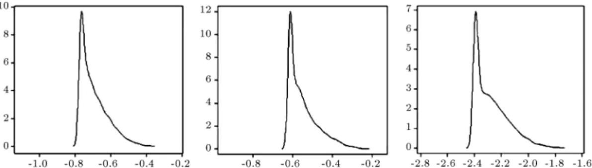
Figure 2. The density of some of the estimated entries in the precision matrix for the cell-signaling data after the 10,000 MCMC iterations, where the rst 2,000 runs take place in the burn-in period. PIP2-PIP3, Plcy-PIP2, and Raf-Mek in lexicographical order.
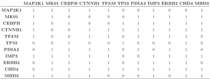
Table 4. The adjacency matrix of the ovarian cancer data estimated by the 10,000 RJMCMC iterations, where the rst 2,000 runs take place in the burn-in period.
MAP2K1 MK01 CEBPB CTNNB1 TFAM TP53 PDIA3 IMP3 ERBB2 CHD4 MBD3
MAP2K1 1 1 1 1 1 1 1 1 1 1 1
MK01 1 1 1 1 1 1 1 1 1 1 1
CEBPB 1 1 1 1 1 1 1 1 1 1 1
CTNNB1 1 1 1 1 1 1 1 1 1 1 1
TFAM 1 1 1 1 1 1 1 1 1 1 1
TP53 1 1 1 1 1 1 1 1 1 1 1
PDIA3 1 1 1 1 1 1 1 1 1 1 1
IMP3 1 1 1 1 1 1 1 1 1 1 1
ERBB2 1 1 1 1 1 1 1 1 1 1 1
CHD4 1 1 1 1 1 1 1 1 1 1 1
MBD3 1 1 1 1 1 1 1 1 1 1 1
on the 2,000 runs taking place the burn-in period, we obtain F1-score as F1-score = 0.63, where T P = 8,
F P = 10, and F N = 11. Eight nodes, found by our codes compatible with the true network, include Raf-Mek, Erk-Raf-Mek, PIP2-PLCY-, PIP3-PIP2, Erk-Akt, Erk-PKA, Raf-PKC, and PKC-Mek. The density plots of the estimated links after the burn-in are also shown in Figure 2. On the other hand, the values of the birth-and-death algorithm are computed as F1-score =
0.50, while T P = 7, F P = 1, and F N = 13. Based on these outputs, it is seen that RJMCMC enjoys better accuracy than the birth-and-death method for this dataset.
3.3. Ovarian cancer data
In this analysis, we specically deal with gynecologic cancer including the ovarian, cervix, and endometrial cancers. This type of cancer is the second most prevalent cancer in women in the world after breast cancer. In our study, we initially search the biological literature and detect 11 core genes, which are active in gynecologic cancer [15-17]. These genes are named as MPK2K1, MK01, CEBPB, CTNNB1, TFAM, TP53,
PDIA3, IMP3, ERBB2, CHD4, and MBD3. Then, based on the ArrayExpress database, an Aymetix dataset is considered and collected under the ovarian cancer, and the observations belonging to the underly-ing 11 genes are selected.
In the data, each gene has 14 samples and the true network composed of these genes is complete, i.e., its adjacency matrix has the value of one in all entries. The estimated adjacency matrix from RJMCMC and BDMCMC is presented in Tables 4 and 5, respectively. In the estimation, similar to previous analyses, 10,000 MCMC iterations are conducted, and the rst 2,000 runs are discarded in the burn-in period. From the outcomes, we calculate F1-score = 1 for RJMCMC and
F1-score = 0.79 for BDMCMC. Thereby, as observed
from other analyses, the ndings show that RJMCMC outperforms BDMCMC with higher accuracy.
4. Results and discussion
This study extended the idea of the Copula GGM (CGGM) model in the description of biological net-works since GGM is one of the successful probabilistic
Table 5. The adjacency matrix of the ovarian cancer data estimated by the 10,000 BDMCMC iterations, where the rst 2,000 runs take place in the burn-in period.
MAP2K1 MK01 CEBPB CTNNB1 TFAM TP53 PDIA3 IMP3 ERBB2 CHD4 MBD3
MAP2K1 1 1 1 1 1 0 0 1 0 0 1
MK01 1 1 0 0 0 0 1 1 1 1 1
CEBPB 1 0 1 0 0 1 1 1 1 1 1
CTNNB1 1 0 0 1 1 1 1 1 1 1 1
TFAM 1 0 0 1 1 0 1 1 1 1 0
TP53 0 0 1 0 0 1 0 0 0 1 0
PDIA3 0 1 1 1 1 0 1 0 1 1 0
IMP3 1 1 1 1 1 0 0 1 1 1 1
ERBB2 0 1 1 1 1 0 1 1 1 1 0
CHD4 0 1 1 1 1 1 1 1 1 1 1
MBD3 1 1 1 1 0 0 0 1 0 1 1
modeling approaches for explaining the steady-state behavior of the biological systems, and the copulas enable us to separate any high-dimensional joint func-tion as marginals. Hereby, CGGM can be also used instead of sole GGM, especially for high-dimensional systems as it can partition the high-dimensional joint density into small parts, resulting in simplicity of esti-mating the model parameters. In the inference of the underlying model, the Reversible Jump Markov Chain Monte Carlo (RJMCMC) approach as another alterna-tive to the birth-and-death (BDMCMC) algorithm for CGGM is implemented [9,6]. In the computation, the RJMCMC approach has been adopted to estimate the biological networks by writing all codes as the open-source R codes and making all necessary calibrations in the calculations while converting the implementation of these techniques into the system's biology. In the application, the bench-mark Rochdale dataset is used and applied to compare dierent modeling and inference approaches in the system's biology to validate the performance of the current calculation. Then, we have also implemented it for the inference of the cell signaling pathway and the ovarian cancer data. Ac-cording to the comparative analyses via the BDMCMC algorithm [9,6], we have observed that RJMCMC gives more accurate results in all analyses.
As the extension of this study, the split-merge method [19] and the Gibbs sampling [8] are used as the new alternatives to RJMCMC in selecting the dimension for the precision matrix. Because even though these listed methods have been also suggested in place of RJMCMC theoretically, their application to real-life and high-dimensional network problems has not been performed yet. Further, although the accu-racy of RJMCMC is signicantly high, its calculation via R can be computationally demanding. Hereby, any improvement in the selection procedure of the precision matrix can be deemed useful to deal with
the existing challenge during the computational time. The construction of complex systems via CGGM with RJMCMC or its new alternates can help us describe the actual biological activations better and identify any malfunctions in the systems that cause illnesses.
Furthermore, RJMCMC has been performed for Time Series CGGM (TSCGGM) [1] so that the mea-surement based on dierent time-course data [20,21] can be applied to estimate the biological networks. In this model, we are interested in estimating two matrices: the precision matrix and the autoregressive coecient matrix. The last one shows time dependency between variables in the vector autoregression VAR(1) modeling, which can be extended to VAR(p) by our recommended method. In the study of Abegaz and Wit (2013) [22], this calculation is done via the penalized likelihood approach to the state space model. In addition, we think that this model can be extended by using the vine rather than the Gaussian copulas [23,24]. In doing so, the strict normality assumption of the measurements can be relaxed by accepting other non-normal distributions. Because, in some cases, the normality assumption or the normalization of the data can dissemble the structure, particularly in dealing with a sample of lower size, which is a common challenge in biological datasets. This question is one of the major interests in computational and systematic biology whose applications can be seen from various biological sciences, ranging from genetics to pharma-cology.
Furthermore, another powerful alternate to RJM-CMC in inference of the relationship between variables can be a Multivariate Adaptive Regression Spline (MARS), which is, in brief, a non-parametric regression technique and can be seen as an extension of linear models that automatically describe nonlinearities and interactions between variables. From previous studies, it has been shown that RJMCMC can be used in certain
parts of MARS [25], and we think that this idea can be adapted for the construction of biological networks, too. From the recent literature about the MARS model, it has been found that the conic version of MARS, called CMARS [26,27], and its robustication, called robust CMARS or shortly RCMARS [28,29], are two other extended versions of MARS to improve the accuracy of the nonlinear and correlated data. Among these alternatives, the CMARS model has been implemented to construct biological networks; based on the results, it has been observed that the accuracy of the model can increase in comparison to the MARS model [30]. Moreover, the CMARS model is also extended by dierent bootstrapping regression methods to obtain the empirical distributions of the parameters of CMARS [31]. In addition, Yerlikaya-Ozkurt et al. (2016) [32] and Taylan et al. (2014) [33] developed a new scheme to minimize the impact of outliers on regression estimators of CMARS. On the other hand, the RCMARS model was applied to build a precipitation model of the continental central Anatolia region of Turkey [34]. Then, it is also performed for the presentation of the regulatory networks [35]. However, the performance of this model has not been compared yet with CGGM in terms of accuracy and evaluation of the computational demand of dierent biological systems' models. It is supposed here that such a comparative study can be useful for detecting the most accurate model that, particularly, t with protein-protein interaction data.
Furthermore, all these models from CGGM, MARS, CMARS, and RCMARS, which can describe the steady-state activation of the biological systems, can be extended by considering the randomness in the nature of the systems. Under this condition, the stochastic models can be benecial. Among alterna-tives, the diusion model [36], the discretized version of the diusion model [37-40], and the Stochastic Hy-brid Systems (SHS) [41] are implemented in modeling biological networks. In these models, SHS is further extended by adding jumps to describe the abrupt changes in the data [42,43], whereas the application of this model to biological networks and the Bayesian inference of this jump model have not been studied yet. Hereby, the application of this approach to signal transaction data has been considered, and an attempt has been made to adapt RJMCMC for this model. In the end, such a novelty in SHS can open new avenues for the representation of the biological systems under stochastic models.
Acknowledgements
The authors would like to thank the TUB_ITAK (The Scientic and Technological Research Council of Turkey) grant (Project no: 114E636) for their support
and would like to thank Prof. Dr. Alexander R. de Leon for his helpful discussion and insights. Moreover, the authors would like to thank anonymous referees and the editors of the journal for their constructive comments and recommendations, which improved the readability and quality of the paper.
References
1. Whittaker, J. Graphical Models in Applied Multivari-ate Statistics, John Wiley and Sons, New York (1990). 2. Friedman, J., Hastie, T., and Tibshirani, R. \Sparse inverse covariance estimation with the graphical lasso", Biostatistics, 9, pp. 432-441 (2008).
3. Meinshausen, N. and Buhlmann, P. \High dimensional graphs and variable selection with the lasso", The Annals of Statistics, 34, pp. 1436-1462 (2006). 4. Green, P.J. \Reversible jump Markov chain Monte
Carlo computation and Bayesian model determina-tion", Biometrika, 82(4), pp. 711-732 (1995).
5. Dobra, A. and Lenkoski, A. \Copula Gaussian graphi-cal models and their application to modeling functional disability data", Annals of Applied Statistics, 5, pp. 969-993 (2011).
6. Mohammadi, A. \Bayesian model determination in complex systems", PhD Thesis. University of Gronin-gen, Netherland (2015).
7. Richardson, S. and Green, P.J. \Bayesian analysis of mixtures with an unknown number of components", Journal of Royal Statistical Society B, 59, pp. 731-792 (1997).
8. Walker, S. \A Gibbs sampling alternative to reversible jump MCMC", Report no.: IMS-EJS-EJS 2009 383, pp. 1-3 (2009).
9. Mohammadi, A. and Wit, E.C. \Bayesian struc-ture learning in sparse Gaussian graphical models", Bayesian Analysis, 10, pp. 109-138 (2015).
10. Skrondal, A. and Rabe-Hesketch, S. \Structural equa-tion modeling: Categorical variables", Entry for the Encyclopedia of Statistics in Behavioral Science, Wi-ley, pp. 1-8 (2005).
11. Wang, H. and Zhengzi, S. \Ecient Gaussian graphical model determination under G-Wishart prior distribu-tions", Electronic Journal of Statistics, 6, pp. 168-198 (2012).
12. Lenkoski, A. \A direct sampler for G-Wishart vari-ates", Statistics, 2, pp. 119-128 (2013).
13. Atay-Kayis, A. \A Monte Carlo method for computing the marginal likelihood in non-decomposable Gaussian graphical models", Biometrika, 92(2), pp. 317-335 (2005).
14. Ai, J. \Reversible-jump MCMC methods in Bayesian statistics", MSc Thesis, The University of Leeds, United Kingdom (2012).
15. Hu, Z., Zhu, D. etc. \Genome-wide proling of HPV in-tegration in cervical cancer identies clustered genomic hot spots and a potential microhomolgy-mediated integration mechanism", Nature Genetics, 47(2), pp. 158-163 (2015).
16. The Cancer Genome Atlas Research Network. \In-tegrated genomic analyses of ovarian Carcinoma", Nature, 474, pp. 609-615 (2011).
17. Levine, D.A. and The Cancer Genome Atlas Research Network \Integrated genomic characterization of en-dometrial carcinoma", Nature, 497, pp. 67-73 (2013). 18. Sachs, K., Perez, O., Pe'er, D., Lauenburger, D.A.,
and Nolan, G.P. \Causal protein-signaling networks derived from multiparameter single-cell data", Science, 308, pp. 523-529 (2005).
19. Trivedi, P.K. and Zimmer, D.M. \Copula modeling: An introduction for practitioners", Foundations and Trends R in Econometrics, 1, pp. 1-111 (2005). 20. Weber, G.W., Defterli, O., Alparslan Gok, S.Z., and
Kropat, E. \Modeling, inference and optimization of regulatory networks based on time series data", European Journal of Operational Research, 211(1), pp. 1-14 (2011).
21. Sima, C., Hua, J., and Jung, S. \Inference of gene regulatory networks using time-series data", A Survey, Current Genomics, 10(6), pp. 416-429 (2009). 22. Abegaz, F. and Wit, E. \Sparse time series chain
graphical models for reconstructing genetic networks", Biostatistics, 14(3), pp. 586-599 (2013).
23. Wawrzyniak, M.M. \Dependence concepts", MSc The-sis, Delft University of Technology, Netherland (2006). 24. Brechmann, E.C. and Schepsmeier, U. \Modeling de-pendence with C- and D-vine copulas: The R package CDVine", Journal of Statistical Software, 52(3), pp. 1-27 (2013).
25. Holmes, C.C. and Denison, D.G.T. \Classication with Bayesian MARS", Machine Learning, 50, pp. 159-173 (2003).
26. Yerlikaya- Ozkurt, F., CMARS: A New Contribution to Nonparametric Regression with MARS, Lap Lambert Academic Publishing (2011).
27. Weber, G.W., Batmaz, _I., Koksal, G., Taylan, P., and Yerlikaya- Ozkurt, F. \CMARS: a new contribution to nonparametric regression with multivariate adaptive regression splines supported by continuous optimiza-tion", Inverse Problems in Science and Engineering, 20(3), pp. 371-400 (2012).
28. Ozmen, A. Robust Optimization of Spline Models and Complex Regulatory Networks, Springer International Publishing, Switzerland (2016).
29. Ozmen, A., Weber, G.W., Batmaz, _I., and Kropat, E. \RCMARS: Robustication of CMARS with dif-ferent scenarios under polyhedral uncertainty set", Communications in Nonlinear Science and Numerical Simulation, 16(12), pp. 4780-4787 (2011).
30. Ayyldz, E., Purutcuoglu, V., and Weber, G.W. \Loop-based conic multivariate adaptive regression splines is a novel method for advanced construction of complex biological networks", European Journal of Operational Research, 270(3), pp. 852-861 (2018). 31. Yazc, C., Yerlikaya- Ozkurt, F., and Batmaz, _I. \A
computational approach to nonparametric regression: bootstrapping CMARS method", Machine Learning, 101(1-3), pp. 211-230 (2015).
32. Yerlikaya- Ozkurt, F., ASkan, A., and Weber, G.W. \A hybrid computational method based on convex optimization for outlier problems: Application to earthquake ground motion prediction", Informatica, 27(4), pp. 893-910 (2016).
33. Taylan, P., Yerlikaya- Ozkurt, F., and Weber, G.W. \An approach to the mean shift outlier model by Tikhonov regularization and conic programming", In-telligent Data Analysis, 18(1), pp. 79-94 (2014). 34. Ozmen, A., Kropat, E., and Weber, G.W. \Robust op-
timization in spline regression models for multi-model regulatory networks under polyhedral uncertainty", Optimization, 66(12), pp. 2135-2155 (2017).
35. Ozmen, A., Batmaz, _I., and Weber, G.W. \Precip- itation modeling by polyhedral RCMARS and com-parison with MARS and CMARS", Environmental Modeling and Assessment, 19(5), pp. 425-435 (2014). 36. Bower, J. and Bolouri, H., Computational Modeling
of Genetic and Biochemical Networks, MIT Press, London (2001).
37. Golightly, A. and Wilkinson, D.J. \Bayesian inference for stochastic kinetic models using diusion approxi-mation", Biometrics, 61(3), pp. 781-788 (2005). 38. Golightly, A. and Wilkinson, D.J. \Bayesian sequential
inference for stochastic kinetic biochemical network models", Journal of Computational Biology, 13(3), pp. 838-851 (2006).
39. Purutcuoglu, V. \Inference of stochastic MAPK path-way by modied diusion bridge method", Central European Journal of Operational Research, 21(2), pp. 415-429 (2013).
40. Purutcuoglu, V. and Wit, E. \Bayesian inference for the MAPK/ERK pathway by considering the depen-dency of the kinetic parameters", Bayesian Analysis, 3(4), pp. 851-886 (2008).
41. Li, X., Omotere, O., Qian, L., and Dougherty, E.R. \Review of stochastic hybrid systems with applica-tions in biological systems modeling and analysis", EURASIP Journal on Bioinformatics and Systems Biology, 8, pp. 1-12 (2017).
42. Savku, E. \Advance in optimal control of markov regime-switching models with applications in nance and economics", PhD Thesis. Middle East Technical University, Turkey (2017).
43. Savku, E., Azevedo, N., and Weber, G.W. \Optimal control of stochastic hybrid models in the framework of regime switches", Modeling, Dynamics, Optimization and Bioeconomics, II. Editors: Pinto, A. and Zilber-man, D., Springer, pp. 371-387 (2017).
Biographies
Hajar Farnoudkia (1986) is a PhD student of Statis-tics at Middle East Technical University (METU) since 2015. She received her MSc and BSc degrees from the University of Tabriz. Her research interests include Gaussian graphical models and their application to biological datasets. She is currently working on time series chain graphical models and C-vine and D-vine copulas.
Vilda Purutcuoglu is a Professor at the
Depart-ment of Statistics at Middle East Technical University (METU) and also aliated faculty in the Informatics Institute, Institute of Applied Mathematics and De-partment of Biomedical Engineering at METU. She has completed her BSc and MSc in Statistics and holds minor degree in Economics. She received her doctorate from the Lancaster University. Dr. Purutcuoglu's cur-rent research interests lie in the eld of bioinformatics, systems biology, and biostatistics. She has a research group who has been working on deterministic and stochastic modeling of biological networks and their inferences via Bayesian and frequentist theories.
![Table 1. The lexicographical ordered Rochdale data [7].](https://thumb-us.123doks.com/thumbv2/123dok_us/8368381.2222530/5.892.233.682.803.1154/table-the-lexicographical-ordered-rochdale-data.webp)