Statistical Methods for Imaging Genetic Data
Ja-an Lin
A dissertation submitted to the faculty of the University of North Carolina at Chapel Hill in partial fulfillment of the requirements for the degree of Doctor of Philosophy in the Department of Biostatistics.
Chapel Hill 2013
Approved by:
Dr. Hongtu Zhu
Dr. Joseph G Ibrahim
Dr. Rebecca Santelli
Dr. Wei Sun
c
2013
Ja-an Lin
Abstract
JA-AN LIN: Statistical Methods for Imaging Genetic Data (Under the direction of Dr. Hongtu Zhu )
Table of Contents
List of Tables . . . viii
List of Figures . . . xi
1 Introduction . . . 1
1.1 Literature Review . . . 1
1.1.1 Multivariate Linear Model . . . 2
1.1.2 Component-wise Method . . . 3
1.1.3 Principle Component Analysis . . . 3
1.1.4 Partial Least Square Regression . . . 4
1.1.5 Sparse Reduced Rank Regression . . . 4
1.1.6 Least Square Kernel Machine Method . . . 5
1.2 Introduction to our approach . . . 7
2 Projection Regression Method . . . 10
2.1 Methods . . . 10
2.1.2 Test Procedure for Testing Hypotheses . . . 16
2.1.3 Summary . . . 17
2.2 Results . . . 18
2.2.1 Simulation Studies . . . 18
2.2.2 A neonatal study . . . 20
2.2.3 Tables and Figures . . . 23
3 Functional Mixed Effects Model - FMEM . . . 31
3.1 Methods . . . 31
3.1.1 Two-stage Estimation Procedure . . . 33
3.2 Results . . . 39
3.2.1 Simulation Studies . . . 39
3.2.2 ADNI Data Analysis . . . 42
3.2.3 Tables and Figures . . . 47
4 Score Test for Functional Mixed Effects Model . . . 55
4.1 Method . . . 55
4.1.1 Weighted Score Test Statistic . . . 55
4.1.2 Adaptive Estimation for Weight and Neighborhood . . . 58
4.2 Results . . . 62
4.2.1 Simulation Studies . . . 62
4.2.2 ADNI Data Analysis . . . 65
4.2.3 Tables and Figures . . . 69
5 Conclusion . . . 74
Appendix I: Additional Results for PRM . . . 76
Appendix II: Supplementary Tables and Additional Results of FMEM . 84 Appendix III: Proof of (3.11) . . . 92
Appendix IV: Derivation of Weighted Score Test of FMEM . . . 96
List of Tables
2.1 Selected SNPs with the corresponding genes and result for testing a single SNP effect while adjusting for demographic information and other SNPs 30
3.1 The estimation results of σ2
γ(v) in Scenario I using FMEM and voxel-wise method in terms of average absolute value of bias (BIAS), root mean squares (RMS), standard deviation (SD), and the ratio between RMS and SD (RE). . . 51 3.2 The estimation results ofσ2
γ(v) inScenario II by using FMEM and voxel-wise method in terms of average absolute value of bias (BIAS), root mean squares (RMS), standard deviation (SD), and the ratio between RMS and SD (RE). . . 52 3.3 The dice overlap ratio (DOR), average number of false positive cluster,
and average size of false positive cluster for Scenario I with different cluster size thresholds. . . 52 3.4 The dice overlap ratio (DOR), average number of false positive cluster,
and average size of false positive cluster for Scenario II with different cluster size thresholds. . . 53
3.5 The global power calculation of number of significant voxels detected by voxel-wise approach and FMEM in both scenarios. . . 54
4.1 The dice overlap ratio (DOR), average number of false positive cluster, and average size of false positive cluster for Scenario I with different cluster size thresholds. . . 71 4.2 The dice overlap ratio (DOR), average number of false positive cluster,
and average size of false positive cluster for Scenario II with different cluster size thresholds. . . 71
4.3 The global power calculation of number of significant voxels detected by voxel-wise approach and FMEM in both scenarios. . . 72 4.4 Demographic information of the selected 206 subjects. For thecategorical
A1.1 Type I Errors - Part 1 . . . 76
A1.2 Type I Errors - Part 2 . . . 77
A1.3 Type I Errors - Part 3 . . . 78
A1.4 Type I Errors - Part 4 . . . 79
A1.5 Power - Part 1 . . . 80
A1.6 Power - Part 2 . . . 81
A1.7 Power - Part 3 . . . 82
A1.8 Power - Part 4 . . . 83
A1.9 P-values from PCA method to analyze neonatal data . . . 83
A2.1 Descriptive statistics of SNRs for 10 regions of σ2 γ(v) from a simulated data of scenario I, in which the SNPs are extracted from the chromosome 1 in ADNI. . . 84
A2.2 Descriptive statistics of SNRs for 10 regions of σ2γ(v) from a simulated data set of scenario II, in which the SNPs are extracted from the gene PICALM in ADNI. . . 85
A2.3 The minor allele frequency (MAF) in % of selected SNPs on TOMM40, PICALM, CR1 and CD2AP . . . 86
A2.4 Demographic information of the 328 subjects in the dataset investigating the effects of PICALM. For the categorical variables: gender, hand-edness and risk of APOE, the numbers are the frequencies for the corre-sponding groups. For thecontinuous variables: baseline age, baseline ICV and years of education, the numbers are the mean (standard deviation) for the corresponding groups. . . 87
A2.5 Demographic information of the 299 subjects in the dataset investigating the effects of CD2AP. For the categorical variables: gender, handedness and risk of APOE, the numbers are the frequencies for the corresponding groups. For the continuous variables: baseline age, baseline ICV and years of education, the numbers are the mean (standard deviation) for the corresponding groups. . . 88
A2.7 The detailed significant brain regions affected byCR1using FMEM. The regions with the ∗ means the regions are detected by FMEM and voxel-based method; the regions with the∗∗means only detected by voxel-based method;• means not applicable. . . 90 A2.8 The detailed significant brain regions affected byPICALMusing FMEM.
List of Figures
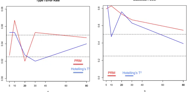
2.1 The comparison results of the PRM and Hotelling’s T2 test based on N = 150 and MAF=0.5: the type I error (the left panel) and power
(the right panel). The upper and middle dashed lines in the left panel correspond to 0.05 and 0.025, respectively; and the upper and middle dashed lines in the right panel represent 0.5 and 0.25, respectively. . . . 23 2.2 Thetype I error comparison results of the PRM, CWM, and PCR
meth-ods based on different sample sizes (150, 200, 250 and 300) and different
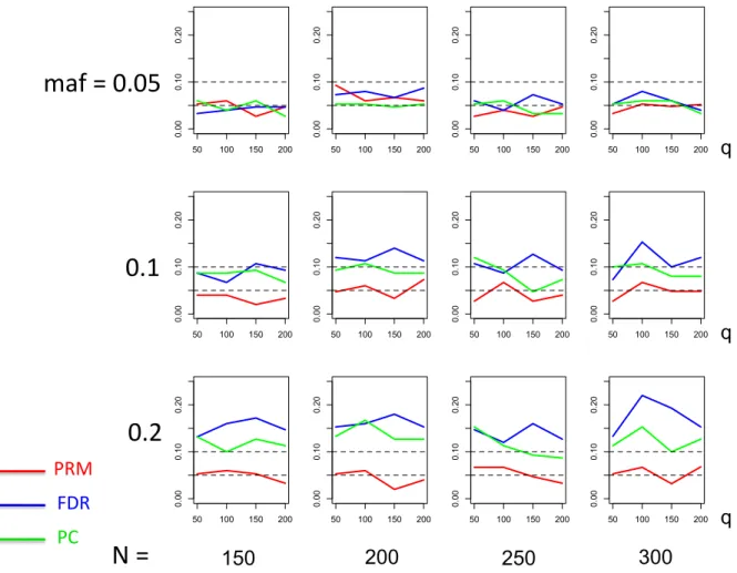
minor allele frequencies (0.05, 0.1 and 0.2). The horizontal axis of each plot is the number of phenotypesqand thevertical axis is the type I error rate. The upper and middle dashed lines are 0.1 and 0.05, respectively. . 24 2.3 Thetype I error comparison results of the PRM, CWM, and PCR
meth-ods based on different sample sizes (150, 200, 250 and 300) and different
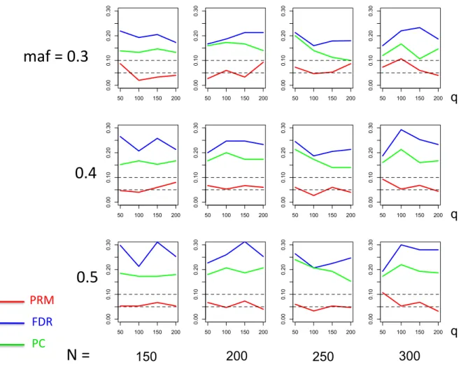
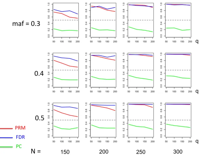
minor allele frequencies (0.3, 0.4 and 0.5). The horizontal axis of each plot is the number of phenotypesqand thevertical axis is the type I error rate. The upper and middle dashed lines are 0.1 and 0.05, respectively. . 25 2.4 The power comparison results of the PRM, CWM, and PCR methods
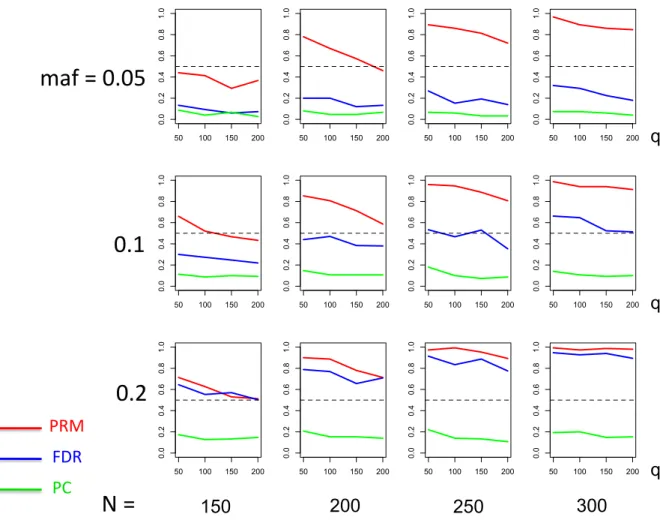
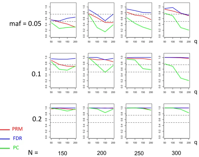
for the first scenario of sparse SNP effect based on different sample sizes (150, 200, 250 and 300) and different minor allele frequencies (0.05, 0.1 and 0.2). Thehorizontal axis of each plot is the number of phenotypes q
and the vertical axis is the power. The dashed line represents a power of 50%. . . 26 2.5 The power comparison results of the PRM, CWM, and PCR methods
for the first scenario of sparse SNP effect based on different sample sizes (150, 200, 250 and 300) and different minor allele frequencies (0.3, 0.4 and 0.5). Thehorizontal axis of each plot is the number of phenotypes q
and the vertical axis is the power. The dashed line represents a power of 50%. . . 27 2.6 The power comparison results of the PRM, CWM, and PCR methods
for multiple SNP effects based on different sample sizes (150, 200, 250 and 300) and different minor allele frequencies (0.05, 0.1 and 0.2). The
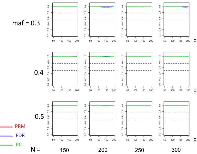
2.7 Thepower comparison results of the PRM, CWM, and PCR methods for the second scenario of multiple SNP effects based on different sample sizes (150, 200, 250 and 300) and different minor allele frequencies (0.3, 0.4 and 0.5). The horizontal axis of each plot is the number of phenotypes
q and the vertical axis is the power. The upper and lower dashed lines represent the powers of 75% and 50%, respectively. . . 29
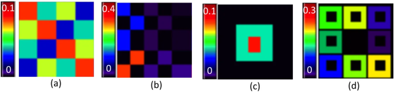
3.1 Simulation setting: (a) True image of β0; (b) true image of β1, in which
the colors represent the values of β1(v)×104; (c) true image of β2; and
(d) true image of β3. . . 47
3.2 Simulation results for estimation accuracy: Scenario I : (a) estimated
σ2
γ(v) by using voxel-wise approach; (b) true σγ2(v) image; and (c) esti-matedσγ2(v) by using FMEM. Scenario II : (d) estimated σγ2(v) by using
voxel-wise approach; (e) true σ2
γ(v) image; (f) estimated σ2γ(v) by using
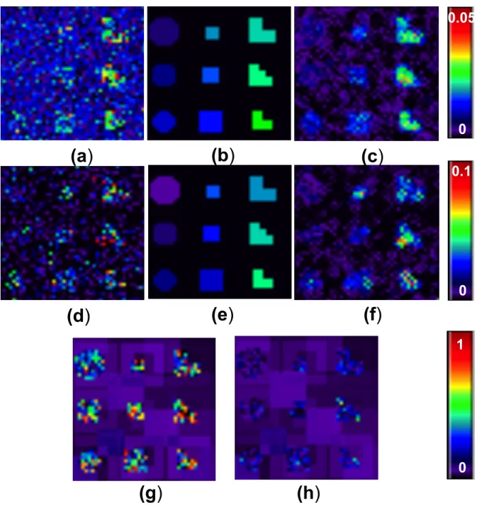
FMEM. Signal to noise ratio (SNR) images for (g) Scenario I and (h) Scenario II . . . 48 3.3 Simulation results for testing the genetic effect: Scenario I: the
rejec-tion rate image at a selected slice by using (a) voxel-wise approach and (b) FMEM; Scenario II: the rejection rate image by using (c) voxel-wise
approach and (d) FMEM. . . 49 3.4 ADNI data analysis: the −log10(p) map of testing the genetic effect of
CD2AP on RAVEN images by using FMEM from 12 selected slices. . . 50
4.1 Simulation setting. True σ2
γ(v) image (a) Scenario I and (b) Scenario II; signal to noise ratio (SNR) images for (c) Scenario I and (d) Scenario II. 69 4.2 Simulation results for testing the genetic effect: Scenario I: the rejection
rate image at a selected slice by using (a) regular score test and (b)
weighted score test; Scenario II: the rejection rate image by using (c)
regular score test and (d) weighted score test. . . 70 4.3 ADNI data analysis: the −log10(p) map of testing the genetic effect of
Chapter 1
Introduction
1.1 Literature Review
There are six commonly used approaches to delineate the association between the phe-notypes and gephe-notypes.
1.1.1 Multivariate Linear Model
A standard statistical approach to this problem is to fit a multivariate linear model (MLM) to the multivariate phenotype with the candidate genotypes. The mathematical form of the MLM is usually formulated as
Yn×q=Xn×pBp×q+En×q, (1.1)
where n is the total number of subjects, p is the number of covariates including geno-types, q is the dimension of phenotype, each row of the matrices Y,X and E are the phenotype, covariates and random errors for a subject, respectively. With the normality and independence assumption, to test the effect of a single covariate to the whole pheno-type, typically Hotelling’sT2 has been used to test hypotheses of interest [Chung et al., 2010; Taylor and Worsley, 2008; Worsley et al., 2004]. Suppose the null hypothesis is formulated as H0 : Cq×1B =b0, where b0 is a constant. The Hotelling’s T2 statistic is
calculated as
T2 = n−p−q+ 1 (n−p)q (C
ˆ
B−b0)TCov\(CB) −1
(CBˆ −b0), (1.2)
1.1.2 Component-wise Method
An alternative approach is to fit a marginal linear model and calculate a test statistic for each component of the multivariate phenotype. Then it combines all tests with their associated p−values to test an overall hypothesis across all individual phenotypes and adjusting for multiple comparison [Heller et al., 2007; Lazar et al., 2002]. The commonly used adjustment are Bonferroni correction, false discovery rate (FDR) and random field theory (RFT) if the multivariate phenotype is a whole brain image. The Bonferroni correction controls for over all familywise error rate. The FDR controls the expected portion of falsely discovered p-values. Random field theory gives a threshold considering the spatial correlation of the image by involving the imaging smoothness and image size, to cut of p-values.Besides the potential estimation bias due to ignorance of the potential correlation among all individual phenotypes, Bonferroni correction suffers from low statistical power and FDR has inflated type I errors
1.1.3 Principle Component Analysis
1.1.4 Partial Least Square Regression
Partial least squares regression (PLSR) is another statistical method that finds a linear regression model by projecting the multivariate phenotype and the explanatory variables to a new and smaller space [Chun and Keles, 2010; Krishnan et al., 2011]. Conceptu-ally, PLSR is trying to find the multidimensional direction in the phenotype space that explains the maximum variance direction in the phenotype space. Suppose we have a MLM model for the multivariate phenotype and covariates of interest with the no-tations following (1.1). The PLSR is implemented by extracting factors from both X
and Y such that covariance between the extracted factors is maximized. Pratically, the following underlying model is assumed:
X=T PT +E (1.3)
Y =U QT +F, (1.4)
where T and U are two n ×l matrices representing the scores similar to the PCs in PCA framework and P and Q are the loadings in the similar context. E and F are unexplained part. PLSR tries to achieve its goal by maximizing the covariance between
T and U. However, this method focuses on prediction and classification, instead of investigating the association between the multivariate phenotype and the covariates of interest.
1.1.5 Sparse Reduced Rank Regression
dependence of the phenotype on the genotype such that
Y =XB=XW A+E (1.5)
where the notation follows (1.1), W is thep×rmatrix of regression coefficients for thep
genotypes, and Ais ther×q matrix of regression coefficients for theq phenotype, both of full rankr. The factorization of the regression coefficient matrixB =W Acomes from imposing a reduced rank condition onC, namely that rank(C) isr ≤min(p, q). To find out the regulating genotypes to the phenotype, the sRRR model further involves a L1
penalty on each column of regression coefficients. Although it may successfully identify the activation voxels, it still does not account for the spatial correlation in phenotypes as well as the LD structure in genotypes only the representing genotype will be selected by L1 penalty instead of a group of regulation genotypes. The other drawback of this
approach is its incapableness of performing hypothesis testing.
1.1.6 Least Square Kernel Machine Method
Another group of approaches use lease square kernel machine to accommodate the LD structure of a group of genes when investigating the relationship between imaging phe-notype and a group of genetic information. In Liu et al. [2007], they assume for thei-th subject, the univariate response of interest yi can be modeled by
yi =xTi β+h(zi) +ei, (1.6)
h(•) are estimated via maximizing the scaled penalized likelihood function
J(h, β) =−0.5 n
X
i=1
yi−xiβ−h(zi)−0.5λkhk2HK (1.7)
By assuming the function h(•) in the space HK generating by K(•,•), h(•) can be represented as
h(•) = n
X
i=1
αiK(•, zi), (1.8)
where α = (α1,· · ·, αn)T are unknown parameters. The representing form leads the objective function (1.7) becomes
J(h, β) = −0.5 n
X
i=1
yi−xiβ−h(zi)−0.5λαTKα, (1.9)
whereK is a n by n matrix with the (i, j)-th element as K(zi, zj). The normal equation to solve the parameters β and α of (1.9) is the same as the linear mixed model
y=Xβ+h+e, (1.10)
when solving for β and h where β is a p by 1 vector of regression coefficient, h is an n by 1 vector of random effects with distribution N(0, τK), and e ∼ N(0, σ2I). With this connection between (1.8) and (1.10), it is sufficient to test the integrated effect of genetic variation to the response of interest y by testing the null hypothesis
H0 : τ = 0 using sophisticatedly developed linear mixed model theory. Moreover, this
model enables considering the LD structure among a group of genetic variation even when the dimension is high. In Ge and et al [2012], it applies LSKM to structure imaging responses that they repeatedly fit the model (1.6) for each voxel following with testing the null hypothesis H0 : τ = 0 for overall genetic effect and then apply random field
1.2 Introduction to our approach
There is a trend in imaging genetics which utilizes phenotype-wide and genome-wide approaches [Hibar and et al, 2011; Shen et al., 2010; Stein et al., 2010; Ge and et al, 2012]. The standard approach is to repeatedly fit statistical models for each voxel by each genome or gene. Besides computational burden , there are some other limitations. First, the p-values of significant genomes at each nearby voxel may have different order, which makes the biological interpretation complicated. Second, some imaging measures are affected by the interaction between genomes rather than a single genome, which results in missing identification of such genomes. Last, the spatial coherence and spatially contiguous region of activation are not considered in voxel-wise approach thus causing statistical power loss.
of a group of genetic markers, we model the genetic effects as population-shared random effects with a common variance component (VC), whereas to accommodate spatial fea-ture in imaging data, we spatially model varying associations between imaging measures in a three-dimensional (3D) volume (or 2D surface) with a set of covariates and the ge-netic random effects. Moreover, we assume that the varying associations are piecewise smooth functions with unknown edges and jumps across voxels. We develop a two-stage estimation procedure to spatially and adaptively estimate the varying coefficient func-tions. Each stage of the estimation procedure includes a multiscale adaptive estimation and testing procedure to independently estimate each varying coefficient function, while preserving its edges among different piecewise-smooth regions. Simulation studies and real data analysis show that FMEM significantly outperforms voxel-wide approaches in terms of both type I and II error rates. However, with wild-bootstrap method in hy-pothesis testing , the computation is intensive for FMEM. In our third work, we enhance the computational method by revising the weighted likelihood ratio test to the weighted score test which gives comparable statistical power to identify activation regions with more efficient computation. In the weighted likelihood ratio test, the statistical power is enhanced by providing more accurate estimation of VC which results in smaller variance of test statistic. However, the rationale in weighted score test is different that the detail is described in later section.
Chapter 2
Projection Regression Method
2.1 Methods
Suppose that we observe aq×1 multivariate phenotypeyi = (yi1, . . . , yiq)T and ap×1 vector of covariates of interest xi = (xi1, . . . , xip)T for i = 1, . . . , N. We consider a commonly used MLM as follows:
Y =XB+E, or yi =BTxi+ei, (2.1)
whereY is anN×q matrix formed by theq×1 multivariate phenotype of each subject in each row, X is an N ×p matrix consisting of the p×1 vector of covariates of each subject in each row, andB = (βjl) is ap×q matrix, in whichβjl represents the effect of the j−th covariate on the l−th response. Moreover, E is an N ×q matrix representing the random errors and eTi is the i−th row of E with zero mean and covariance matrix
VR. Assuming that xi and ei are independent, the covariance ofyi is given by
Cov(yi) = VQ+VR =BTCov(xi)B+VR, (2.2)
where VQ represents the variation coming from the covariates of interest.
ques-tions can often be formulated as linear hypotheses ofB as follows:
H0 :CB=B0 v.s. H1 :CB6=B0, (2.3)
where Cis a r×pmatrix of full row rank and B0 is a p×q vector of constants.
We consider a projection of yi via a q ×k weight matrix W and create a k ×1 projection vector WTy
i such that k << q. Then, we propose a projection regression model (PRM) given by
WTyi =βwTxi+εi, (2.4)
where βw is a p× k regression coefficient matrix and εi is the random vector with Cov(εi) = Σi. The PRM (2.4) is a heteroscedastic multivariate linear model. When k = 1 and Σi = Σ for all i, PRM reduces to the pseudo-phenotype model considered in [Amos et al., 1990, Amos and Laing, 1993, Ott and Rabinowitz, 1999, Lange et al., 2004, Klei et al., 2008]. A direct connection between models (2.1) and (2.4) is that model (2.1) can be rewritten as
WTyi =βwTxi+εi = (BW)Txi+WTei. (2.5)
Therefore, if W in (2.4) were known, then one would directly perform an appropriate hypothesis test to address specific research hypotheses as follows:
H0W :Cβw=b0 v.s. H1W :Cβw6=b0, (2.6)
where b0 is an r×k vector of constants. Based on model (2.5), the null hypothesis of
(2.6) can be written as Cβw =CBW =B0W=b0.
Let C1 be a (p−r)×p matrix such that
Let D = [CT CT
1]T be a p×p matrix and ˜xi = (˜xTi1,x˜Ti2) = D −Tx
i be a p×1 vector, where ˜xi1 and ˜xi2 are, respectively, ther×1 and (p−r)×1 subvectors of ˜xi. We define
˜
B = [ ˜BT
1B˜T2]T to be ˜B = DB or B = D
−1B˜. We consider ˜B = [ ˜BT
1B˜T2]T, where ˜B1
and ˜B2 are, respectively, the firstr rows and the last p−rrows of B. Therefore, model
(2.5) can be rewritten as
WTyi = (D−1BW˜ )Txi +WTei =WTB˜T1x˜i1+WTB˜2Tx˜i2+WTei. (2.8)
The next issue is to determine an optimalq×kmatrixWunder some certain criteria. In PCH [Ott and Rabinowitz, 1999; Lange et al., 2004; Klei et al., 2008], the heritability ratio is defined by
h(w) = w TV
Qw wTCov(y
i)w
= w
TV Qw wTV
Qw+wTVRw
. (2.9)
The heritability ratio characterizes the ratio of the variation from the genetic biomarkers
xi to the total variation of responses yi. Maximizing h(w) leads to the optimal W.
Instead of directly using the heritability ratio h(w), we consider a generalized ‘heri-tability’ ratio H(w) for a given q×1 vector w as follows:
H(w) = w TB˜T
1Cov(˜xi1) ˜B1w wTV
Rw
. (2.10)
TheH(w) can be interpreted as the ratio of the variance of wTB˜T
1x˜i1 relative to that of wTe
i under the null hypothesis. We require that the optimalW enhances the power of detecting the association betweenWTy
i and xi for the null hypothesis (2.6). Thus, we need to find a W to project the data into a space containing the most information on the null hypothesis of (2.3). Let ΣX = Cov(x). It can be shown that ˜H(w) reduces to
˜
H(w) = w
TBTCT(D−TΣ
XD−1)(1,1)CBw wTV
Rw
where (D−TΣ
XD−1)(1,1) is the upperr×r submatrix of D−TΣXD−1. When C= [Ir0], ˜
H(w) reduces to the ratio of wTBT
1(ΣX)(1,1)B1w to wTVRw, in which (ΣX)(1,1) is the
upper r×r submatrix of ΣX.
When VR is positive definite, maximizing (2.11) is equivalent to maximizing
˜
H(w) = w
TLL−1BTCT(D−TΣ
XD−1)(1,1)CB(L−1)TLTw
wTLLTw , (2.12)
where L is the lower triangular matrix obtained from the Cholesky decomposition of
VR =LLT. Letting VC,X =L−1BTCT(D−TΣXD−1)(1,1)CB(L−1)T. Let v be the
eigen-vector corresponding to the largest eigenvalue of the matrix VC,X, then (2.11) is max-imized when LTwˆ equals v. Hence, (2.12) is maximized when wˆ equals L−Tv. If q is relatively small compared to N, based on (2.11), we take the q×k matrix W in (2.4) by choosing the largest k sparse eigenvectors of VC,X using PCA. However, when q is relatively large compared to N, calculating L−T and the eigenvectors of V
C,X can be challenging, which makes the optimal weight matrix W very unstable.
2.1.1 Estimation Procedure for Optimal Weights
We develop an estimation procedure for estimating the optimal weights. This procedure consists of three major steps: (i) a pre-screening process for eliminating ‘unrelated’ mea-sures; (ii) a shrinkage procedure for approximatingVC,X andVR; and (iii) a sparse prin-cipal component analysis (SPCA) procedure for calculating the eigenvalue-eigenvector pairs of VC,X. Each step is implemented as follows.
The pre-screening procedure is to rank individual phenotypes according to marginal utility and eliminate ‘unrelated’ phenotypes whenq is relatively large relative to N, say
pheno-types and the covariates of interest. In Step 2, we calculate the corresponding Wald-type test statistics under the same null hypothesis (2.6), and the respective p-values from a chi-square distribution with degrees of freedomrfor each individual phenotype. In Step 3, after ordering the q p-values from the smallest to the largest, we only select the phe-notypes with the first q∗ = [q/log(q)] + 1 if q ≤ N, or the first q∗ = [N/log(N)] + 1 if
q > N, where [x] represents the largest integer smaller than x. Thus, we set the weights for those unselected individual phenotypes to be zero, or equivalently, we consider a reduced response vector, denoted asy∗i = (˜yi1, . . . ,y˜iq∗)T orY∗.
The shrinkage procedure is to approximate VC,X and VR as follows. In Step 1, we refit the multivariate linear regression in (2.1) with the selected individual phe-notypes in y∗i as responses conditional on X. Let B∗ be the regression parameter matrix for the selected individual phenotypes. We estimate B∗ by its least square estimator, denoted by ˆB∗, which equals ˆB∗ = (XTX)−1XTY∗. In Step 2, we esti-mate Cov(X) by using its empirical estimator, denoted by ˆΣX, and then approximate VB = BTCT(D−TΣXD−1)(1,1)CB by VcB = ˆB∗TCT(D−TΣXD−1)(1,1)CBˆ∗. In Step 3,
we calculate a shrinkage estimate of VR by following Ledoit and Wolf [2004]. Let CE be the sample covariance matrix of ˆE∗ = (rjk) = Y∗ −XBˆ∗, µE = q−1tr(CE) and ρ= min(1, N−2PN
i=1tr[(ˆeiˆeTi −CE)2]/tr[(CE −µEIq)2]), in which ˆei =y∗i −Bˆ∗Txi. Fi-nally, we approximateVR andVC,X by using ˆVR,S =ρµEIq+ (1−ρ)CE and Lb−1VbB(Lb−T),
respectively. We use ˆVR,S mainly due to its computational efficiency and relatively nice properties [Ledoit and Wolf, 2004].
calculate the loadings of the first k ordinary principal components of ˆVR,S, denoted as α. In Step 2, given a fixed α, we solve the following naive elastic net problem: for
j = 1, . . . , k,
ˆ
γj = argmin γ∗ γ
∗T
( ˆVR,S+λ2,j)γ∗−2αjTVˆR,Sγ∗+λ1,j |γ∗ |1, (2.13)
where | · |1 denotes the L1 norm. Moreover, λ1,j and λ2,j are tuning parameters and selected simultaneously by using a BIC-type selection criterion [Leng and Wang, 2009]. We calculate the BIC-type criterion given by
BIC = (αj−γˆj)TVˆR,S(αj −ˆγj) +df(λ1,j,λ2,j)×
log(q∗)
q∗ , (2.14)
wheredf(λ1,j,λ2,j) is the number of nonzero coefficients in ˆγj. In Step 3, for each fixed ˆγj, we calculate the singular value decomposition of ˆVR,Sγˆj =U DVT, and then we update αj =U VT forj = 1, . . . , k. In Step 4, we repeat steps 2-3, untilγ converges. In Step 5, we normalize γ, and then set ˆvj =γj/|γj | for j = 1, . . . , k. The optimal weight wj is estimated by using ˆwj = (Lb−T)ˆvj forj = 1, . . . , k and W= [w1, . . . ,wk].
2.1.2 Test Procedure for Testing Hypotheses
We develop several statistics of testing H0W againstH1W for the PRM (2.4) as follows. Given the estimated weight matrix W, we can calculate the ordinary least squares estimate of βw, given by ˆβw = (PNi=1xixTi )
−1PN
i=1xiy T
i W. Subsequently, to calculate a statistic for testing H0W againstH1W, we calculate a k×k matrix, denoted by TN, as follows:
TN = (Cβˆw−b0)TΣΩ−1˜ (Cβˆw−b0), (2.15)
where ΣΩ˜ is a consistent estimate of the covariance matrix of Cβˆw−b0 given by
ΣΩ˜ =C(XTX)−1 N
X
i=1
a2ixi˜iT˜ixTi (X TX)−1
CT. (2.16)
Moreover,ai = 1/{1−xTi (XTX)−1xi}and ˜i =WTyi−β˜wTxi, where ˜βwis the restricted
least squares (RLS) estimate ofβ under H0, and is given by
˜
βw = ˆβw−(XTX)−1CT[C(XTX)−1CT]−1(Cβˆw−b0). (2.17)
Whenk = 1,TN is a Wald-type (or Hotelling’sT2) test statistic. Whenk > 1, we define three test statistics based on the functionals of TN as follows:
WN = det(TN), TrN = trace(TN), and RoyN = max(eig(TN)), (2.18)
where det, trace, and eig denote the determinant, trace and eigenvalues of a symmetric matrix, respectively. When k = 1, all these statistics reduce to TN. For simplicity, we focus on TrN throughout the paper.
We present a wild bootstrap method to improve the finite sample performance of the test statistic TrN in (2.18) in testing the null hypothesis H0. First, we fit model
coefficients under (2.3), denoted by B∗b , with corresponding residuals ˆei = yi −BbT∗xi
for i = 1, . . . , N. Then, we generate G bootstrap samples {(zi(g),xi) : i = 1, . . . , N} as follows:
z(ig) =BbT∗xi+η
(g)
i eˆi for i= 1, . . . , N, (2.19)
where η(ig) are independently and identically distributed as a distribution d, in which d
is chosen as
η(ig) =
1, with probability 0.5,
−1, with probability 0.5.
(2.20)
For each generated wild-bootstrap sample, we repeat the estimation procedure for esti-mating the optimal weights and the calculation of the test statistic Tr(Ng). Subsequently, the p-value of TrN is computed as
PG
g=11(Tr (g)
N ≥ TrN)/G, where 1(·) is an indicator function.
2.1.3 Summary
We summarize the key steps of the PRM as follows:
Step (i). Fit q marginal linear regression models with the univariate dependent variable as each single phenotype and the independent variables as the covariates of interest.
Step (ii). Calculate q Wald-type test statistics under the same null hypothesis (2.6) and their corresponding p-values.
Step (iii). Select the responses with the smallest [log(qq)+1] = q∗ (or [log(nn)+1] = q∗
if n≤q)p-values and establish the shrunken response space Y∗; Step (iv). Apply SPCA to estimate the weight W based on Y∗; Step (v). ProjectY toWTY and regress WTY by X;
Step (vii). Generate G bootstrap samples and repeat Steps (i) to (vi) for each bootstrap sample;
Step (viii). Approximate the p-value of TrN.
2.2 Results
2.2.1 Simulation Studies
We carried out two scenarios of simulation studies to examine the finite-sample perfor-mance of the PRM. The simulation studies were designed to establish the association between a relatively high-dimensional phenotype with a commonly used genetic marker (e.g., SNP), while adjusting for age and other environmental factors. The first scenario focuses on that q is relatively smaller than the sample size N. The second scenario focuses on that q is comparable to the sample size N.
150 and the number of wild bootstrap samples to be 250.
Scenario I
In the first scenario, we set the sample size N to be 150 and the MAF to be 0.5. The q
were chosen to be 5, 10, 20, 30, 80 and 100, respectively. The first five individual phe-notypes were associated with the SNP, whose coefficients were independently generated from a normal distribution with mean 0.15 and variance 0.05, and the 5th phenotype was also associated with disease status with regression coefficient being 0.5. We applied both the PRM and Hotelling’s T2 test to each simulated dataset in order to examine the type I and II error rates under the 5% significance level. Inspecting Figure 1 reveals that the type I errors are well controlled for both methods. Moreover, as q increases, the power in detecting the SNP effect decreases faster for Hotelling’s T2 test compared
with the PRM.
Scenario II
set the regression coefficient for the diagnosis status to be 0.5 for the 10th individual phenotype and all other regression coefficients to be zero.
We applied the PRM to the simulated data sets and compared it with two other methods including a component wise method (CWM) and a principal components regression (PCR) using a 5% significance level. The CWM method fits a single linear regression to each individual phenotype with the same set of covariates and uses the false discovery rate (FDR) to test the additive SNP effect. The PCR method extracts the first three principal components of the multivariate phenotype by using the PCA and then fits a multivariate linear model to the extracted principal components with the same set of covariates. The Hotelling’s T2 test is not considered here since it is invalid for q > N.
We observe that the type I error rates are well controlled and more stable in the PRM, compared to the CWM and PCR methods (Figures 2 and 3). When the SNP effect is sparse, the powers of the PRM are generally higher than the CWM method, particularly for SNPs with small MAF and it is uniformly better than the PCR method (Figures 4 and 5). As expected, increasing either the sample size N or the MAF enhances the statistical power in detecting the SNP effect, whereas increasing the number of responses
q reduces the power in detecting the SNP effect. When more SNPs show impact on the phenotypes, PRM is still comparable to CWM and better then PCR when the MAF is small (Figures 6 and 7). With increasing MAF, all three methods perform equally well.
2.2.2 A neonatal study
images were collected with a Siemens head-only 3T scanner using a 3D spoiled gradient (FLASH TR/TE/Flip Angle 15/7msec/25 ˆAˇr) with spatial resolution 1 x 1 x 1 mm3
voxel size. There are 47 regions of interest defined from the T1-weighted images by non-linear warping of a parcellation atlas template [Gilmore et al., 2007; Knickmeyer et al., 2008]. The demographic information includes gender, gestational age at birth in days, age after birth in days and intracranial volume (ICV) of the infants. There are 128 male and 109 female infants with average gestational age 264.0 (SD ±18.91), age after birth in days of 30.2 (SD ±17.80) and ICV 481799.9 (SD ±61528.96). Moreover, 9 genetic variants expressed in SNPs from 6 genes were collected and genotyped by Genome Quebec using Sequenom iPLEX Gold Genotyping Technology.
We applied our PRM method to multivariate phenotype including the volumes of 47 regions of interest (ROIs) with covariates of interest including gender, gestational age, age after birth, ICV and the 9 SNPs with an additive effect. Each hypothesis tests a single SNP effect, while adjusting for other covariates including demographic information and other SNPs. We list the 9 SNPs with their corresponding genes and respective p-values in Table 1.
The results show that the SNPs rs6675281 and rs35753505 have a significant impact on early age brain development with p-values of 0.016 and 0.0136, respectively. This agrees with the existing literature. Specifically, DISC1 was known to be associated with mental illness, such as schizoprenia and bipolar disorder, and NRG1 was known to relate to brain tissue volume [Mata et al., 2009].
supplementary document. When analyzing the same data set by CWM with multiple comparisons adjusted by FDR, none of the 9 SNPs are detected to be significant for the 47 ROIs at the same testing level.
2.2.3 Tables and Figures
20 40 60 80
0.00
0.02
0.04
0.06
0.08
Type I Error Rate
q
5 10 20 30 80 20 40 60 80
0.0
0.2
0.4
0.6
0.8
Statistical Power
q
5 10 20 30 80
PRM
Hotelling’s T2
PRM Hotelling’s T2
50 100 150 200
0.00
0.10
0.20
50 100 150 200
0.00
0.10
0.20
50 100 150 200
0.00
0.10
0.20
50 100 150 200
0.00
0.10
0.20
50 100 150 200
0.00
0.10
0.20
50 100 150 200
0.00
0.10
0.20
50 100 150 200
0.00
0.10
0.20
50 100 150 200
0.00
0.10
0.20
50 100 150 200
0.00
0.10
0.20
50 100 150 200
0.00
0.10
0.20
50 100 150 200
0.00
0.10
0.20
50 100 150 200
0.00
0.10
0.20
N =
maf = 0.05
0.1
0.2
PRMFDR PC
q
q
q
150 200 250 300
50 100 150 200
0.00
0.10
0.20
0.30
50 100 150 200
0.00
0.10
0.20
0.30
50 100 150 200
0.00
0.10
0.20
0.30
50 100 150 200
0.00
0.10
0.20
0.30
50 100 150 200
0.00
0.10
0.20
0.30
50 100 150 200
0.00
0.10
0.20
0.30
50 100 150 200
0.00
0.10
0.20
0.30
50 100 150 200
0.00
0.10
0.20
0.30
50 100 150 200
0.00
0.10
0.20
0.30
50 100 150 200
0.00
0.10
0.20
0.30
50 100 150 200
0.00
0.10
0.20
0.30
50 100 150 200
0.00
0.10
0.20
0.30
N =
maf = 0.3
0.4
0.5
PRMFDR
PC
q
q
q
150 200 250 300
Figure 2.3: Thetype I error comparison results of the PRM, CWM, and PCR methods based on different sample sizes (150, 200, 250 and 300) and different minor allele fre-quencies (0.3, 0.4 and 0.5). Thehorizontal axis of each plot is the number of phenotypes
50 100 150 200 0.0 0.2 0.4 0.6 0.8 1.0
50 100 150 200
0.0 0.2 0.4 0.6 0.8 1.0
50 100 150 200
0.0 0.2 0.4 0.6 0.8 1.0
50 100 150 200
0.0 0.2 0.4 0.6 0.8 1.0
50 100 150 200
0.0 0.2 0.4 0.6 0.8 1.0
50 100 150 200
0.0 0.2 0.4 0.6 0.8 1.0
50 100 150 200
0.0 0.2 0.4 0.6 0.8 1.0
50 100 150 200
0.0 0.2 0.4 0.6 0.8 1.0
50 100 150 200
0.0 0.2 0.4 0.6 0.8 1.0
50 100 150 200
0.0 0.2 0.4 0.6 0.8 1.0
50 100 150 200
0.0 0.2 0.4 0.6 0.8 1.0
50 100 150 200
0.0 0.2 0.4 0.6 0.8 1.0
N =
maf = 0.05
0.1
0.2
PRMFDR PC
q
q
q
150 200 250 300
50 100 150 200 0.0 0.2 0.4 0.6 0.8 1.0
50 100 150 200
0.0 0.2 0.4 0.6 0.8 1.0
50 100 150 200
0.0 0.2 0.4 0.6 0.8 1.0
50 100 150 200
0.0 0.2 0.4 0.6 0.8 1.0
50 100 150 200
0.0 0.2 0.4 0.6 0.8 1.0
50 100 150 200
0.0 0.2 0.4 0.6 0.8 1.0
50 100 150 200
0.0 0.2 0.4 0.6 0.8 1.0
50 100 150 200
0.0 0.2 0.4 0.6 0.8 1.0
50 100 150 200
0.0 0.2 0.4 0.6 0.8 1.0
50 100 150 200
0.0 0.2 0.4 0.6 0.8 1.0
50 100 150 200
0.0 0.2 0.4 0.6 0.8 1.0
50 100 150 200
0.0 0.2 0.4 0.6 0.8 1.0
N =
maf = 0.3
0.4
0.5
PRM
FDR PC
q
q
q
150 200 250 300
50 100 150 200 0.0 0.2 0.4 0.6 0.8 1.0
50 100 150 200
0.0 0.2 0.4 0.6 0.8 1.0
50 100 150 200
0.0 0.2 0.4 0.6 0.8 1.0
50 100 150 200
0.0 0.2 0.4 0.6 0.8 1.0
50 100 150 200
0.0 0.2 0.4 0.6 0.8 1.0
50 100 150 200
0.0 0.2 0.4 0.6 0.8 1.0
50 100 150 200
0.0 0.2 0.4 0.6 0.8 1.0
50 100 150 200
0.0 0.2 0.4 0.6 0.8 1.0
50 100 150 200
0.0 0.2 0.4 0.6 0.8 1.0
50 100 150 200
0.0 0.2 0.4 0.6 0.8 1.0
50 100 150 200
0.0 0.2 0.4 0.6 0.8 1.0
50 100 150 200
0.0 0.2 0.4 0.6 0.8 1.0
N =
maf = 0.05
0.1
0.2
PRM
FDR
PC
q
q
q
150 200 250 300
50 100 150 200 0.0 0.2 0.4 0.6 0.8 1.0
50 100 150 200
0.0 0.2 0.4 0.6 0.8 1.0
50 100 150 200
0.0 0.2 0.4 0.6 0.8 1.0
50 100 150 200
0.0 0.2 0.4 0.6 0.8 1.0
50 100 150 200
0.0 0.2 0.4 0.6 0.8 1.0
50 100 150 200
0.0 0.2 0.4 0.6 0.8 1.0
50 100 150 200
0.0 0.2 0.4 0.6 0.8 1.0
50 100 150 200
0.0 0.2 0.4 0.6 0.8 1.0
50 100 150 200
0.0 0.2 0.4 0.6 0.8 1.0
50 100 150 200
0.0 0.2 0.4 0.6 0.8 1.0
50 100 150 200
0.0 0.2 0.4 0.6 0.8 1.0
50 100 150 200
0.0 0.2 0.4 0.6 0.8 1.0
N =
maf = 0.3
0.4
0.5
PRMFDR PC
q
q
q
150 200 250 300
Table 2.1: Selected SNPs with the corresponding genes and result for testing a single SNP effect while adjusting for demographic information and other SNPs
Gene Abbreviation SNP P-value
Catechol-O-methyltransferase COMT rs4680 0.88
Disrupted-in-schizophrenia-1 DISC1 rs821616 0.75
rs6675281 0.016
Neuregulin 1 NRG1 rs35753505 0.0136
rs6994992 0.51
Estrogen Receptor Alpha ESR1 rs9340799 0.44
rs2234693 0.57
Brain-derived Neurotrophic Factor BDNF rs6265 0.60
Chapter 3
Functional Mixed Effects Model - FMEM
3.1 Methods
Suppose that we observe imaging measures, clinical variables, and genetic markers from
nunrelated subjects. LetV be the whole brain andv be a voxel inV. For each individual
i(i= 1, . . . , n), aNV ×1 vector consisting of imaging measures is observed and denoted by Yi = {yi(v) : v ∈ V}. For notational simplicity, we only consider univariate image measure and thus, NV equals the number of voxels in V. Moreover, a K ×1 vector of clinical covariates xi = (xi1,· · · , xiK)T and an G×1 vector gi = (gi1,· · · , giG)T for genetic data are also collected for each individual. For instance, imaging measures can be the shape representation of the surfaces of cortical or subcortical structures [Chung et al., 2008; Zhu et al., 2007], and genetic makers can be various polymorphism types, such as single nucleotide polymorphisms (SNPs), block substitutions, and copy number variants [Liu et al., 2007; Tzeng and Zhang, 2007; Wang and Chen, 2012].
Our FMEM consists of a mixed effects model (MEM) at each voxel and a jumping surface model (JSM) for varying coefficient functions across the brain. First, at each voxel v inV, MEM is given by
yi(v) = xTi β(v) +h(gi;v) +ei(v) = xTi β(v) +zTiγ(v) +ei(v) for i= 1,· · ·, n, (3.1)
genetic random effects, zi is a pre-specified L×1 vector of functions of gi, and ei(v) is the measurement error. We assume thatei(v)∼N(0, σe(v)2),γ(v)∼N(0, σγ2(v)Γ), and
{ei(v) :v ∈ V} are independent across i and independent of γ(v) for all v ∈ V, where Γ is an L×L identity matrix. Without loss of generality, we assume Γ =IL.
Model (3.1) can be regarded as an alternative representation of variance component models used in the literature [Liu et al., 2007; Tzeng and Zhang, 2007; Kang et al., 2010; Wang and Chen, 2012]. For instance, for the kernel machine framework [Liu et al., 2007], we can directly represent h(gi;v) as the random weighted sum of a set of L orthonormal basis functions by using the Karhunen Loeve expansion. For a given voxel v, the covariance between two individuals i and j are σ2
γ(v)zTi zj. Moreover, for two different voxels v and v0 in V, we assume Cov(γ(v), γ(v0)) = σγ(v)σγ(v0)ργ(v, v0)IL and Cov(ei(v), ei(v0)) = σe(v)σe(v0)ρe(v, v0), where ργ(v, v0) and ρe(v, v0), respectively, characterize the spatial correlation between the genetic random effects and that between the measurement errors. Therefore, for any two voxelsv andv0, the covariance structure of yi(v) is given by
Σy,i(v, v0) = Cov(yi(v), yi(v0)) = σγ(v)σγ(v0)ργ(v, v0)zTi zi+σe(v)σe(v0)ρe(v, v0). (3.2)
We propose JSM for the genetic varying coefficient function {σ2
covariates may play different roles in characterizing the piecewise-smooth pattern of the imaging data.
3.1.1 Two-stage Estimation Procedure
We propose a two-stage estimation procedure to estimate all varying coefficient functions and test their effects on imaging phenotypes. The key ideas of each stage are given as follows:
Stage (I). Spatially and adaptively estimate {σ2
γ(v) : v ∈ V} and test the null hypothesisσγ2(v) = 0 across all voxels.
Stage (II). Directly apply the multiscale adaptive regression models (MARM) in [Li et al., 2011] to spatially and adaptively estimateβ ={β(v) :v ∈ V} and then test associated hypotheses.
Since our primary interest lies in the genetic effect, we focus on Stage (I) and omit Stage (II) for the sake of space.
Stage I
The first stage consists of three major steps as follows:
Step (I.1). Calculate the restricted maximum likelihood (REML) estimator of
η(v) = (σ2
γ(v), σe2(v)) across all voxelsv ∈ V.
Step (I.2). Spatially and adaptively re-estimate {σγ2(v) :v ∈V} by incorporating information from neighboring voxels.
In Step (I.1), we calculate the REML estimator of η(v) across voxels. Let Z = (z1,· · · ,zn) be an L×n matrix, Y(v) = (y1(v),· · ·, yn(v))T be an n ×1 vector, and X = (x1,· · · ,xn) be a p×n matrix. There exists an (n−p)×n matrix Kx such that KxXT =0 and rank(Kx) =n−p. A MEM forY∗(v) =KxY(v) is given by
Y∗(v) = KxZTγ(v) +KxE(v), (3.3)
where E(v) = (e1(v),· · · , en(v))T. Based on the distributional assumptions in (3.1), we have Y∗(v) ∼ N(0,ΣY∗(v)), where ΣY∗(v) = σ2γ(v)KxZTZKxT +σ2e(v)KxKxT. Thus, at
each voxel v, the REML estimate of ˆη(v), denoted by ˆη(v), is to maximize the REML function given by
`REM L(Y∗(v)|Z, η(v)) =−0.5 log|ΣY∗(v)| −0.5Y∗(v)TΣY∗(v)−1Y∗(v). (3.4)
Since our primary interest lies on σγ2(v), we fix σe2(v) as ˆσe2(v) from here on. In Step (I.2), we construct a weighted REML function to estimate σ2
γ(v) by incorpo-rating the spatial information in a neighborhoodB(v, h) for each voxel v with a specific radius h as follows:
LREM L(σ2γ(v)|Y ∗
, B(v, h)) = X v0∈B(v,h)
ωγ(v, v0;h)`REM L(Y∗(v0)|Z, σ2γ(v),σˆ 2 e(v
0
)), (3.5)
where ωγ(v, v0;h) is a weight function of voxels v, v0, and the radiush. Then, we max-imize LREM L(σγ2(v)|Y∗, B(v, h)) to calculate the weighted REML estimator of σ2γ(v), denoted by ˆσγ2(v, h). The weight function ωγ(v, v0;h) measures the data similarity be-tween the two voxels v and v0 such that P
preventing over-smoothing estimation of σ2
γ(v) and preserving the edges of significant regions of{σ2
γ(v) :v ∈ V}.
In Step (I.3), to assess the synthetic genetic effect on imaging phenotype across all voxels, we formulate it as testing the following null and alternative hypotheses:
H0,γ(v) :σγ2(v) = 0 v.s. H1,γ(v) :σγ2(v)>0. (3.6)
We test (3.6) by using the weighted REML ratio statistic defined by
RLRTσ2
γ(v) = 2{LREM L(ˆσ
2
γ(v)|Y
∗, B(v, h))−L
REM L(0|Y∗, B(v, h))}. (3.7)
Since all the subjects share the same random effect γ(v), the standard asymptotic re-sults in Stram and Lee [1994] are invalid and can perform very poorly even for the unweighted REML ratio statistics for testing random effects in model (3.1) [Crainiceanu and Ruppert, 2004]. However, we provide an exact null distribution for RLRTσ2
γ(v) below.
Step (I.2): Adaptive Estimation of σ2 γ(v)
diagram of AET is given as follows:
h0 = 0 < h1 < · · · < hS =r0
B(v, h0) ={v} ⊂ B(v, h1) ⊂ · · · ⊂ B(v, hS)
⇓ ⇓ % · · · % ⇓
{σˆ2
γ(v) :v ∈ V} ⇒ ωγ(v, v0;h1) · · · ωγ(v, v0;hS =r0)
⇓ % · · · % ⇓
{σˆ2
γ(v;h1) :v ∈ V} · · · {σˆ2γ(v;hS) :v ∈ V}.
The key idea of AET is to build a sequence of nested spheresB(v, hs) forh0 = 0 < h1 <
· · · < hS = r0 at each voxel v ∈ V and then sequentially determine ˆσγ(v, v0;hs) for all v0 ∈B(v, hs) based on{σˆγ2(v
0, h
s−1) :v0 ∈B(v, hs)}for all v ∈ V ands= 1, . . . , S. Since the tuning parameters of AET have been described in details in [Polzehl and Spokoiny, 2000; Li et al., 2011], we do not include them here for the sake of brevity.
The three key steps of AET, including weights adaptation, estimation, and termina-tion checking, are presented as follows.
• In the weightsadaption step (i), we select a series{hs =csh :s= 1,· · · , S}of radii with ch ∈ (1,2), say ch = 1.125. We then set s = 1 and h1 = ch. The adaptive weights are given by
ωγ(v, v0;hs) = Kloc(||v−v0||2/hs)Kst(Dγ(v, v0;hs−1)/Cn), (3.8)
where Kloc(u) = (1−u)+ and Kst(u) = min(1,2(1−u2))+ according to previous
experience in the literature [Li et al., 2011], and || · ||2 denotes the Euclidean
norm of a vector (or a matrix). Moreover, Dγ(v, v0;hs−1) is set as {σˆγ2(v;hs−1)−
ˆ
σ2 γ(v
0;h
s−1)}2/var[\σγ2(v)],where var[\σγ2(v)] is estimated by using the inverse of the
Fisher information matrix of (σ2
Li et al. [2011], we choose Cn = n1/3χ2(1)0.5 for Dγ(v, v0;hs−1) defined in (4.13),
whereχ2(1)0.5 is the 0.5-percentile of theχ2(1) distribution. The adaptive weight Kst(Dγ(v, v0;hs−1)/Cn) downweights the role of a voxel v0 ∈B(v, hs) in
LREM L(σγ2(v)|Y ∗
, B(v, hs)) (3.9)
if Dγ(v, v0;hs−1) is large. The weight Kloc(||v−v0||2/hs) gives less weight to the voxel v0 ∈B(v, hs), whose location is far from the voxel v.
• In the estimation step (ii), for each v ∈ V and for the radius hs, we calculate ˆ
σγ(v;hs) by maximizing LREM L(σγ2(v)|Y∗, B(v, h)) defined in equation (3.5) given ωγ(v, v0;hs).
• In the termination checking step (iii), after the S0−th iteration, we calculate a
stopping criterion based on a distance between ˆσ2
γ(v;hS0) and ˆσ 2
γ(v;hs) given by
D( ˆσ2
γ(v;hS0),σˆγ2(v;hs)) ={σˆγ2(v;hS0)−σˆγ2(v;hs)}2var\[σ2γ(v)] −1
(3.10)
fors > S0. Then, we compareD( ˆσγ2(v;hS0),σˆ 2
γ(v;hs)) with a benchmark, denoted by ˜C(s), for s > S0. If D( ˆσγ2(v;hS0),σˆ
2
γ(v;hs)) > C˜(s), then we set ˆσ2γ(v) = ˆ
σ2
γ(v, hs−1) = and the estimation for this voxel v is terminated. If s = S and D( ˆσ2
γ(v;hS0),σˆγ2(v;hs))≤C˜(s), ˆσγ2(v) is set as ˆσγ2(v, hS) and the estimation process terminates. The algorithm stops when the estimation is finished for all v in V. If
s ≤ S0 or D( ˆσ2γ(v;hS0),σˆ 2
γ(v;hs)) ≤ C˜(s) for s < S0 ≤ S −1, then we go back
to the weights adaptation step (i) with an increased radius h = hs+1 = csh+1. Throughout the paper, we set S0 = 2, ˜C(s) =χ2(p)0.7/(s−1), and S = 10.
Step (I.3): Testing H0,γ(v) :σγ2(v) = 0
We perform the hypothesis testing in (3.6) by using the testing statistics RLRTσ2
γ(v) and the corresponding p-values. Let Ω =KxZTZKxT =U D0UT be the spectral
decom-position of Ω such thatD0 = diag(d1,· · · , dn−p) is the diagonal matrix of eigenvaluesdk and U is an (n−p)×(n−p) orthonormal matrix. Without loss of generality, we choose
Kx such that KxKxT =In−p. We obtain the following theorem, whose proof is included in the appendix.
Theorem 1. Under model (3.1), RLRTn(v) can be written as
RLRTn(v)= sup λ(v)≥0
{ X
v0∈B(v,h)
ω(v, v0;h)D(v0;λ(v)/σ2e(v0))}, (3.11)
where λ(v) =σ2
γ(v) and D(v
0;t) is given by
σe−2(v0)Y∗T(v0)Udiag
td1
1 +td1,· · · ,
tdn−p 1 +tdn−p
UTY∗(v0)−
n−p
X
l=1
log(1 +tdl). (3.12)
Moreover, under the null hypothesis H0,γ(v), we have
D(v0;t)=D n−p
X
l=1 δ2
l(v 0)td
l 1 +tdl
−
n−p
X
l=1
log(1 +tdl), (3.13)
where =D means equality in distribution and theδl(v)are i.i.d N(0,1)random variables. Although Theorem 1 provides an efficient way of approximating the null distribution of RLRTn(v), a complex issue arises from the complex spatial correlations among the δ2
l(v
0) across voxels v0 ∈ B(v, h). One approach for dealing with such an issue is to
steps of this bootstrap method are presented in Appendix. After the p-values for all voxels v ∈ V are computed, either a false discovery rate (FDR) method or random field theory (RFT) is applied to correct for multiple comparisons [Ge and et al, 2012].
3.2 Results
3.2.1 Simulation Studies
We simulated data at all NV = 5,808 voxels on a 44×44×3 phantom image. Each z-slice contains the same effect regions. At each voxel, we simulated the univariate imaging measure according to model (3.1) with β(v) = (β0(v), β1(v), β2(v), β3(v))T and
xi = (1, xi1, xi2, xi3)T. Moreover, the covariates xi1, xi2, and xi3 were generated from a
Gaussian distribution with mean 40 and standard deviation 10, a Bernoulli distribution with success probability 0.5, and a Bernoulli distribution with success probability 0.3, respectively. These three covariates were designed to mimic the common clinical vari-ables age, gender, and disease status. For a slice of a phantom image, the effect areas for β0(v) were divided into 16 regions with 4 different values ranging from 0.02 to 0.08,
increasing by 0.02 (Figure 8(a)); forβ1(v), the effect regions were divided into 25 regions ranging from 10−2.5 to 10−12.5, decreasing by a rate of 10−2.5 (Figure 8(b)); forβ
2(v), the
whole space was separated into 3 regions with values 0, 0.05, and 0.1 (Figure 8(c)); the effect area of β3(v) on a slice of phantom image was divided into 9 regions with values
ranging from 0 to 0.1, increasing by differences of 0.025 (Figure 8(d)).
the study period, the subjects were assessed with magnetic resonance imaging (MRI) measures and psychiatric evaluation to determine the diagnosis status at each time point. The genetic information was also collected from each subject at baseline and it is genotyped by the Illumina 610 Quad array with more than 620,000 single nucleotide polymorphysm (SNPs). More information of ADNI is provided in the real data analysis result Section 3.2. We simulated the genetic information based on the two following scenarios.
• Scenario I. To preserve the linkage disequilibrium among SNPs, we utilize all of the SNPs on chromosome 1 from 197 Caucasian controls to generate the genetic effect. After eliminating the SNPs with minor allele frequency (MAF) less than 5%, there were 31554 out of 45627 SNPs left. Then we randomly chose 20 SNPs and 100 subjects among the 197 healthy controls as the simulated genetic datazi in (3.1). In this case, n = 100. If any of these 20 SNPs have MAF less than 5%, the genetic data was resampled until all of the 20 SNPs have MAF ≥5%.
• Scenario II. To evaluate the performance of FMEM in the case of high LD, we selected the SNPs from the same gene in the second scenario. Searching the SNPs on the gene PICALM, which is found to be relevant to Alzheimer’s disease in many studies [Harold et al., 2009] using the gene list “glist-hg18” provided by PLINK, there were 23 SNPs on PICALM with MAF larger than 5%. After eliminating the missing values, there are 176 healthy controls with complete genotype data at these 23 SNPs. We randomly selected 7 SNPs from 75 healthy controls to be zi in (3.1). Although there is strong LD among these 7 SNPs, no SNP has perfect correlation (1 or -1) with any other SNP in these 75 subjects. In this case,nequals 75.
matrix σ2
γ(v)IL. Different σγ2(v) values, which represent different signal-to-noise ratios, were chosen to examine the performance of our method at different signal-to-noise ratios and also to test whether FMEM can perform well for different shapes. See Figure 9 (b) and Figure 9 (e) for Scenarios I and II. Moreover, we overlay some of the effect areas of β3(v) and σ2γ(v) in order to account for the fact that the brain phenotype is an intermediate expression of disease progression. The{σγ2(v) :v ∈ V}of the effect regions in Scenario I were ranging from 0.005 to 0.025, increasing by 0.0025, whereas the{σ2
γ(v) : v ∈ V} of effect regions in Scenario II were ranging from 0.005 to 0.045, increasing by 0.005. The random error ei(v) was independently distributed as a univariate Gaussian distribution with mean 0 and standard deviation 3 for all voxels. We set the number of bootstrap samplesM and the number of repetitions to be 200.
Tables 2 and 3 summarize the estimation results ofσγ2(v) obtained from FMEM and traditional voxel-wise method for both scenarios. It includes the average absolute value of the bias, the root mean square (RMS), standard deviation (SD), and the ratio of RMS over SD. The difference between estimation of RMS and SD is that RMS is estimated using the empirical mean and SD is calculated using theoretical mean. As shown in both tables, FMEM outperforms voxel-wise method with respect to smaller estimation bias which leads to more accurate hypothesis testing conclusion. Note that compared with voxel-wise method, the RMSs and SDs are also smaller for FMEM. This indicates much more stable estimation.
such cluster as a ”true positive”. In contrast, if a specific thresholded cluster does not overlap with any voxels of the 9 effect regions, we call the cluster a “false positive”. We summarized the hypothesis testing results by the average dice overlap ratio (DOR), the average number of false positive clusters, and the average size in the number of voxels of false positive clusters. DOR is the ratio between the number of true positive clusters over the true number of effect areas, which is 9 in this simulation setting. Thus, the higher DOR means the higher the probability of detecting true effect regions. As shown in Tables 4 and 5, if we set the cluster size threshold at 1 voxel, FMEM has smaller DOR and smaller number of false positive clusters compared with voxel-wise method. When the cluster size threshold increases to 10 voxels, FMEM has a similar DOR value as that of the no threshold case, whereas the DOR of the voxel-wise approach reduces by about 20%. Table 6 summarizes the number of significant voxels identified by the two methods in each effect region of Scenarios I and II In Table 6, FMEM identifies less voxels in the non-effect regions, while detecting more voxels in effect regions in both scenarios. Finally, we conclude that FMEM outperforms voxel-wise method in both detecting true effect regions and controlling the false positive error rate.
3.2.2 ADNI Data Analysis
pro-gression of mild cognitive impairment (MCI) and early Alzheimerˆa ˘A´Zs disease (AD). Determination of sensitive and specific markers of very early AD progression is intended to aid researchers and clinicians to develop new treatments and monitor their effective-ness, as well as lessen the time and cost of clinical trials. The Principal Investigator of this initiative is Michael W. Weiner, MD, VA Medical Center and University of Cali-fornia ˆa ˘A¸S San Francisco. ADNI is the result of efforts of many co-investigators from a broad range of academic institutions and private corporations, and subjects have been recruited from over 50 sites across the U.S. and Canada. The initial goal of ADNI was to recruit 800 subjects but ADNI has been followed by ADNI-GO and ADNI-2. To date these three protocols have recruited over 1500 adults, ages 55 to 90, to participate in the research, consisting of cognitively normal older individuals, people with early or late MCI, and people with early AD. The follow up duration of each group is specified in the protocols for ADNI-1, ADNI-2 and ADNI-GO. Subjects originally recruited for ADNI-1 and ADNI-GO had the option to be followed in ADNI-2. For up-to-date information, seewww.adni−inf o.org.
The data we employed to evaluate the performance of FMEM was from the first phase (ADNI), which was conducted mainly to search for the causal SNPs associated with the progression of Alzheimer’s disease and to establish an alternative diagnosis standard using MRI brain images. About 800 subjects with age older than 65 were recruited and followed at least 3 years. The 800 subjects included 200 healthy controls, 400 subjects with different levels of mild cognitive impairment (MCI), and 200 subjects with Alzheimer’s disease (AD). Besides the SNPs and the T1 weighted MRI imaging measurements, the subjects were assessed with demographic information and psychiatric examination scores to determine the diagnosis status at each scheduled visit.
segmentation, and nonlinear registration. After segmentation, the brain was segmented into four different tissues: grey matter (GM), white matter (WM), ventricle (VN), and cerebrospinal fluid (CSF). We quantified the local volumetric group differences by generating RAVENS maps [Davatzikos et al., 2001] for the whole brain and each of the segmented tissue type (GM, WM, VN, and CSF) respectively, using the deformation field we obtained during registration. RAVENS methodology is based on a volume-preserving spatial transformation, which ensures that no volumetric information is lost during the process of spatial normalization, since this process changes an individual0s brain morphology to conform it to the morphology of the Jacob template.
We are interested in detecting meaningful brain regions of interest that are associ-ated with several candidate genes. We included only the subjects whose diagnosis status were healthy control and Alzheimer’s disease at the baseline and had no status change during the study period. After screening, the total number of subjects we included was 372 (195 HCs and 177 ADs). The clinical covariates of interest included in our anal-ysis were gender, baseline age, square of baseline age, handedness, education, baseline intracranial volume, and the risk of APOE. Specifically, the handedness was treated as a binary variable, the education information was the self-reported years of education by the subjects, and the risk of APOE is assumed to be additive. In detail, the risk of APOE for a subject was 3 if he/she carries ε4 at both alleles; it was 2 if he/she carries
ε3 and ε4 in two alleles, the risk would be considered 0 if the two APOE alleles were the combination of ε2 and ε3, and other combination of APOE alleles are assumed to have risk 1.
assembly and is highly correlated with the emergence of late-on-set AD, which is possibly due to the perturbation at synapse triggering its function change [Harold et al., 2009]. The gene CD2AP encodes the CD2-asscociated protein and involves in the process of cell membrane, including endocytosis, that plays critical roles in neurodegeneration and Aβ clearance from the brain [Naj et al., 2011]. The gene CR1 encodes complement component (3b/4b) receptor 1 and the pathways involving CR1 are involved in the AD process, specifically in clearance of Aβ peptides which is the primary composition of amyloid plaques [Lambert et al., 2009].
We first matched the SNPs in ADNI with the gene list “glist-hg18” provided by PLINK [Purcell and et al, 2007] and were able to locate 16, 15, and 23 SNPs on the se-lected CR1, CD2AP, and PICALM genes, respectively. All these SNPs pass the quality control procedure with MAF > 5% and the Hardy Weinberg Equilibrium (HWE) test
p-value> 0.01. The MAFs of SNPs of the selected genes vary from 0.1 to 0.5 and are presented in the supplementary document. After deleting missing values, there are 335, 299 and 328 subjects corresponding to the CR1, CD2AP, and PICALM genes, respec-tively, and their associated demographic information is presented in the supplementary document.
supplementary document, we were able to detect several major ROIs, such as the hip-pocampus, the putamen, and the fusiform. The hippocampus is known to be associated with memory and cognition. The fusiform is associated with color recognition, word and body recognition and the putamen is associated with motor skills. Figure 11 shows the
−log10(p) map of several selected slices with significant clusters for testing the genetic effect of CD2AP on RAVEN images identified by FMEM.
3.2.3 Tables and Figures
(a) (b) (c) (d)
0.1
0
0.4
0
0.1
0
0.3
0
Figure 3.1: Simulation setting: (a) True image of β0; (b) true image of β1, in which the
(a
)
(b
)
(c
)
(d
)
(e
)
(f
)
0
0
0.05
0.1
0
1
(g
)
(h
)
Figure 3.2: Simulation results for estimation accuracy: Scenario I : (a) estimatedσ2 γ(v) by using voxel-wise approach; (b) true σγ2(v) image; and (c) estimated σγ2(v) by using
FMEM. Scenario II : (d) estimated σγ2(v) by using voxel-wise approach; (e) true σγ2(v) image; (f) estimated σ2
γ(v) by using FMEM. Signal to noise ratio (SNR) images for (g) Scenario I and (h) Scenario II
(a)
(b)
(c)
(d)
1
0
Figure 3.3: Simulation results for testing the genetic effect: Scenario I: the rejection rate image at a selected slice by using (a) voxel-wise approach and (b) FMEM; Scenario II: the rejection rate image by using (c) voxel-wise approach and (d) FMEM.
Figure 3.4: ADNI data analysis: the −log10(p) map of testing the genetic effect of
Table 3.1: The estimation results of σ2
γ(v) in Scenario I using FMEM and voxel-wise method in terms of average absolute value of bias (BIAS), root mean squares (RMS), standard deviation (SD), and the ratio between RMS and SD (RE).
FEFM Voxel-based
σ2γ(v) |BIAS| RMS SD RE |BIAS| RMS SD RE
0 0.001 0.002 0.002 1 0.007 0.005 0.005 1
0.005 2.36e-06 0.003 0.003 1 0.005 0.005 0.005 1
0.0075 0.0005 0.003 0.003 1 0.005 0.006 0.006 1
0.01 0.001 0.004 0.004 1 0.006 0.008 0.008 1
0.0125 0.001 0.004 0.004 1 0.006 0.008 0.008 1
0.015 0.002 0.005 0.005 1 0.008 0.010 0.010 1
0.0175 0.003 0.005 0.005 1 0.008 0.010 0.010 1
0.020 0.002 0.006 0.006 1 0.010 0.012 0.012 1
0.0225 0.003 0.006 0.006 1 0.010 0.013 0.013 1
Table 3.2: The estimation results ofσ2
γ(v) inScenario II by using FMEM and voxel-wise method in terms of average absolute value of bias (BIAS), root mean squares (RMS), standard deviation (SD), and the ratio between RMS and SD (RE).
FEFM Voxel-based
σ2γ(v) |BIAS| RMS SD RE |BIAS| RMS SD RE
0 0.002 0.003 0.003 1 0.003 0.008 0.008 1
0.005 0.0001 0.004 0.004 1 0.007 0.126 0.126 1
0.010 0.001 0.006 0.006 1 0.011 0.016 0.016 1
0.015 0.002 0.008 0.008 1 0.014 0.020 0.02 1
0.020 0.002 0.010 0.010 1 0.024 0.017 0.017 1
0.025 0.003 0.020 0.020 1 0.020 0.029 0.029 1
0.030 0.005 0.013 0.013 1 0.023 0.032 0.032 1
0.035 0.004 0.014 0.014 1 0.026 0.035 0.035 1
0.040 0.015 0.006 0.006 1 0.028 0.040 0.040 1
0.045 0.007 0.016 0.016 1 0.031 0.040 0.040 1
Table 3.3: The dice overlap ratio (DOR), average number of false positive cluster, and average size of false positive cluster forScenario I with different cluster size thresholds.
FEFM Voxel-based
Threshold Mean SD Mean SD
Voxel Size = 1
DOR 0.94 0.05 0.99 0.02
False Positive Cluster Number 1.88 6.12 21.30 12.29
False Positive Cluster Size 1.03 0.04 1.06 0.06
Voxel Size = 10
DOR 0.91 0.04 0.83 0.10
False Positive Cluster Number 0 0 0 0
Table 3.4: The dice overlap ratio (DOR), average number of false positive cluster, and average size of false positive cluster forScenario II with different cluster size thresholds.
FEFM Voxel-based
Threshold Mean SD Mean SD
Voxel Size = 1
DOR 0.86 0.06 0.996 0.02
False Positive Cluster Number 1.35 4.85 15.45 12.92
False Positive Cluster Size 1.07 0.08 1.05 0.07
Voxel Size = 10
DOR 0.85 0.07 0.78 0.11
False Positive Cluster Number 0 0 0 0