c
Sharif University of Technology, June 2009
Simulation of a Continuous Thermal Sterilization
Process in the Presence of Solid Particles
A. Shahsavand
1;and Y. Nozari
1Abstract. Simulation of a Continuous Thermal Sterilization (CTS) process is investigated for both laminar and turbulent ow regimes. Various heuristics are considered for the reliable estimation of sterility (F value) and quality (C value) parameters. It is proved that for a laminar condition that using a mixer at the entrance of the holding zone can drastically increase the sterility of food produce, while reducing its quality degradation. For a turbulent ow regime, the eect of trajectories and thermal resistances of solid particles on the performance of the CTS process is investigated. It is clearly shown that the thermal resistances of relatively large particles have a crucial eect on computed values of both sterility and quality parameters.
Keywords: Simulation; Thermal sterilization; Laminar; Turbulent; Lethality; Quality; Solid particles.
INTRODUCTION
Dairy products (such as milk) are suitable environ-ments for the growth of pathological microorganisms and should be carefully sterilized prior to the packaging step, in order to ensure the complete removal of all harmful organisms. Continuous Thermal Sterilization (CTS) and Ultra High Temperature (UHT) processes are traditionally used for this purpose. Various aspects of these processes are explored in this article by resorting to the numerical simulations of CTS and UHT processes.
The rst attempts to model and simulate thermal sterilization processes were carried out in the early seventies [1]. The practical simulations of the thermal sterilization of canned foods were initiated in the 80s and accelerated in the early 90s, due to the signi-cant improvements in computational capability [2-4]. Sudhir K. Sastry presented a comprehensive model for simulation of the CTS process [5]. The practical applicability of the model was severely restricted due to the numerous simplifying assumptions.
In 1993, Zhang and Fryer considered the
simula-1. Department of Chemical Engineering, Faculty of Engineering, Ferdowsi University of Mashhad, Mashhad, P.O. Box 1111, I.R. Iran.
*. Corresponding author. E-mail: [email protected] Received 12 February 2007; received in revised form 22 October 2007; accepted 1 June 2008
tion of a similar process in the presence of the Ohmic heating of a solid-liquid mixture, neglecting the slip velocity between solid and liquid phases [6]. Wadad and Sastry [7] investigated the eect of uid viscosity on the ohmic heating rates of uid-particle mixtures using static, vibrating and ow ohmic heaters. They concluded that in continuous ow heater, the mixture with higher viscosity heats more rapidly. Bapista et al. [8] used a liquid crustal technique to determine average uid-to-particle heat transfer coecients for single spherical hollow aluminum particles heating in carboxymethylcellulose solutions in continuous tube ow.
They reported that for laminar ow conditions of 7 < Reynolds < 284 (144 < Prandtl < 1755), the average values of heat transfer coecients were in the range of 334 and 1497 W/m2C. Fryer [9]
declared that the sterilization rate of canned foods at 140C is about 2000 times faster than at
conven-tional canning temperature of 125C [10]. Since, the
activation energies for the reactions (which result in microbial death) are higher than those which result in quality loss of the food product, therefore the HTST (High-Temperature-Short-Time) processes oer the potential to give the same level of sterility for a reduced quality loss due to severe reduction of retention times [10].
Jung and Fryer [11] presented a meticulous ap-proach in the modeling of the HTST continuous
steril-an indirect type helical tube UHT milk sterilizer. The sterilizer performance was investigated in the temperature range of 90-150C. They declared that
the residence time of the food product can be reduced to a few seconds by keeping the uid at 135-150C.
Using such short residence time maintains cumulative lethality at an allowable level, while preserving the quality of the food product.
Zhong et al. [13] used an infrared camera to record the relatively nonuniform temperature distribu-tion within the small whole carrots, carrot cubes and potato cubes suspended in 1% (w/w) CMC solution when heated by a 40.68 MHz, 30 kW continuous ow Radio Frequency (RF) unit.
Salengke and Sastry [14] investigated the steriliza-tion process of solid-liquid mixture for two previously identies potentially hazardous situations. Once in-volving a particle of electrical conductivity signicantly dierent from its immediate surroundings (inclusion particle) and the other involving a mixed uid. In a separate but very similar paper [15], they modeled the ohmic heating of solid-liquid mixtures under worst-case heating scenarios.
HTST AND UHT PROCESSES
Figure 1 illustrates the three separate sections (heating, holding and cooling zones) of both HTST and UHT processes. The wall temperatures of heating and cooling zones are usually kept constant and the holding tube is always considered adiabatic. The purpose is to maintain an adequate environment in both heating and holding zones for the food product to achieve an allowable level of accumulated sterility (F value). Evidently, the holding time of the UHT process is much less than that for HTST. The uid is nally cooled to preserve its quality (C value).
The amount of accumulated sterility and the corresponding quality destruction depend on the uid temperature prole and its residence time in various zones. For this reason, the temperature and velocity distributions of the food product should be computed prior to any other calculation.
Figure 1. Schematic diagrams of HTST and UHT processes.
MATHEMATICAL MODEL FOR HTST AND UHT PROCESSES
The purpose of this simulation is to compute both ve-locity and temperature proles for laminar and turbu-lent ow regimes. The governing equations (continuity, momentum and energy) are sucient to calculate the required proles for the laminar condition. However, additional equations (such as the k " model presented by Launder and Spalding [16]) are needed to simulate the turbulent process.
Assuming a steady state ow and incompressible uid, the continuity, momentum and energy equations, the heating, holding and cooling zones of a CTS process can be represented in a concise form as follows:
r:v = 0; (1)
r:vv + rp + r: g = 0; (2)
^Cvv:rT = r:q
@p @T
^v(r:v) ( : rv): (3)
Neglecting the gravitational force, the above equations (in the cylindrical coordinate) reduce to the following form for Newtonian uids [17].
@vz
@z = 0; (4)
@p @z +
1 r
@ @r
r@v@rz
^Cpvz@T@z=k:
1 r
@ @r
r@T@r
+@@z2T2
+
@vz
@r 2
: (6) As previously mentioned, the simultaneous solution of Equations 1-3 provides the required temperature and velocity distributions for the laminar CTS process.
However, as shown later, additional equations are necessary to dene the turbulent energy (k) and its dissipation rate (") for a turbulent condition [16].
Evidently, the heating zone dasher (a screw type blade mounted on a shaft to prevent excessive pre-cipitation of solid particles on heat exchanger inner walls) produces a sophisticated velocity prole, which is dicult to include in the above equations. Therefore, the dasher movement and also the thermal resistance of the solid particles are ignored for further simplication. The latter assumption will be relaxed in the last sections of this article.
After computation of temperature and velocity proles in each of the heating, holding and cooling zones of the CTS process, the amount of accumu-lated lethality (F value) and the corresponding quality parameter (C value) can be simply obtained by the following equations [11].
F =
t
Z
0
10(Ti(t) Tref)z dt; (7)
C =
t
Z
0
10(Ti(t) T czc ref)dt: (8)
Since large F values indicate the high sterility of the food products and large C values denote a signicant reduction in the product quality, therefore, the thermal sterilization process should be designed in such a way as to provide maximum required sterility while maintaining the minimum C value.
SIMULATION RESULTS
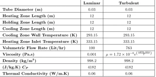
The laminar data set presented in Table 1 is exactly borrowed from Jung and Fryer [11] and the turbu-lent data are practically the same, only corrected for viscosity and the corresponding volumetric ow rate to accommodate for the sharp temperature dierence and to provide a sucient degree of turbulence. Both data sets are used extensively in this article for various simulations of CTS processes.
Laminar Condition
Simulation of the CTS process was performed us-ing both analytical and numerical (nite dierence) methods for the solution of governing Equations 1-3. The analytical solution was derived by Subrama-nian (\The Greatx Problem" (taken from the website: http://www.clarkson.edu/subramanian/ch490/).), ig-noring the conduction heat transfer term in comparison to axial convection. Evidently, the Peclet number (which is the ratio of convectional heat transfer to conduction) should be excessively large (Pe 100) to validate the above assumption [18,19]. Fortunately, using = 10 7 m2/s and data of Table 1, the
corresponding Peclet number will be computed around 10000, which is much greater than the required crite-rion [20].
Since the analytical solution is only available for limited cases, the numerical solution of governing equations was performed using a nite dierence tech-nique. Figure 2 illustrates the remarkable agreement of analytical and numerical solutions for the prediction of various dimensionless temperature distributions. The nite dierence method will be used from now on for simulation of the CTS process in all laminar conditions. Figure 3 shows the temperature distributions of the three sterilization zones under a laminar condition for six dierent radiuses, assuming that the wall
tem-Table 1. Data sets used for simulations.
Laminar Turbulent
Tube Diameter (m) 0.03 0.03
Heating Zone Length (m) 12 12
Holding Zone Length (m) 12 12
Cooling Zone Length (m) 12 12
Cooling Zone Wall Temperature (K) 293.15 293.15
Heating Zone Inlet Temperature (K) 333.15 333.15
Volumetric Flow Rate (Lit/hr) 100 763
Viscosity (Pa.s) 0.001 = 1:72 10 6e(1876:353
T )
Density (kg/m3) 998.2 998.2
(J/kg.K) CP 4182 4182
Figure 2. Comparison of analytical and numerical methods for prediction of temperature proles across the length of heating zone.
Figure 3. Temperature distributions of various laminar layers across all three zones (heating, holding and cooling).
perature of heating zone (TW H) is 140C. Evidently,
the 12-meter holding zone length is sucient to bring the hottest (r R) and coldest (r = 0) layers to thermal equilibrium. However, this does not imply that a necessarily sucient level of sterility is accumulated in the food product. This issue will be considered in more detail in the next sections.
Figure 4 illustrates the excellent agreement of the temperature distributions reported by Jung and Fryer [11] and the predicted ones via the nite dier-ence method. The bulk temperatures are computed using the following denition:
Tb(x) = R
R
0 2rv(r)T (x; r)dr
_Q : (9)
On many occasions, the accumulated sterility of the food product is computed by assuming that the spore or pathogenic particle is located at the center of the entire heating and holding zones. As shown in Figure 3,
Figure 4. Comparison of computed temperature distributions with reported values of Jung and Fryer [9].
the corresponding temperature is the lowest at any section and the center velocity has the highest value for both laminar and turbulent conditions. Evidently, using such a conservative approach can lead to signif-icant over-processing (due to predicting unrealistically small accumulated lethality), and thus unnecessary deterioration of the overall product quality.
This point is considered in more detail in the following section by comparing various strategies for considering dierent temperature and velocity proles to predict sterility (F value) and quality (C value) parameters.
First Method: Employing Exact Temperature and Velocity Distributions
The following equation (presented by Jung and Fryer [11] for a laminar condition) may be used for the calculation of accumulated lethality (average F value) when the exact temperature and velocity proles are known:
F = Dreflog
Nf
N0
= Dreflog
0 B B B B B B @
r
R
02rv(r):10
tsiR 010
(Ti(t) Tref) z dt Dref dr
_Q
1 C C C C C C A ;
(10)
where Dref is the decimal reduction time required to
reduce the initial microorganism population by a factor of 10 at reference temperature (Tref= 121:1C), z is the
temperature change (C) giving a 10-fold dierence in
decimal reduction time, and _Q is the volumetric ow rate of the food product. The average C value is also computed from the following similar equation:
C = DC;reflog
0 B B B B B B B B @
r
R
0 2rv(r):10
tsiR 010
(Ti(t) T Cref) zC dt DC;ref dr
Q
1 C C C C C C C C A :
(11)
Figure 5 compares the values of sterility and quality parameters computed via several dierent strategies for estimating the temperature and velocity (residence time) of the coldest particle (or layer). The solid line represents the exact temperature and velocity distributions and other undemanding approaches are considered in more detail in the following sections. Second Method: Using the Center Temperature and Maximum Velocity
In the most conservative approach, one may consider that the pathogenic particle always travels at the center of the heating and holding tubes. In this case, the minimum temperature and maximum velocity at each section should be used in Equations 7 and 8 for prediction of the sterility and quality parameters. Figure 5 illustrates that such a conservative approach will predict unrealistically small accumulated lethality
Figure 5. Comparison of various methods for prediction of sterility and quality parameters via dierent T & V distributions.
and quality parameters, leading to a very long holding tube length. Evidently, such systems, although main-taining high levels of sterility, result in excessive quality destruction of the food product.
Third Method: Using the Center Temperature and Average Velocity
To prevent unnecessary deterioration of the sterilized product, the residence time can be reduced by using average velocity. Figure 5 shows that, although such an approach calculates sterility values close to the exact (rst) method, the predicted quality reduction of the food product is much lower than the actual value. Fourth Method: Using the Bulk Temperature and Maximum Velocity
In some cases, the bulk temperature of the uid at each section (Equation 9) and the maximum velocity may be used to compute the sterility and quality parameters via Equations 7 and 8. This approach predicts reasonable sterility values but underestimates the quality reduction parameter, as shown in Figure 5. Fifth Method: Using the Bulk Temperature and Average Velocity
Considering the average velocity drastically increases the residence time and, hence, predicts the largest sterility values, as shown in Figure 5. This situation leads to underestimating the length of the holding tube and provides insucient sterility of the food product. The predicted quality reduction is the closest value to the exact (rst) method.
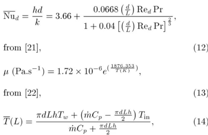
Sixth Method: Using the Bulk Temperature via Nusselt Method
Instead of computing the bulk temperature from Equa-tion 9 (which requires exact temperature and velocity distributions), the following equations can be used simultaneously to calculate the approximate average bulk temperature of the uid between the inlet and any given section (L) of the heating tube.
Nud =hdk = 3:66 + 0:0668 d L
RedPr
1 + 0:04 d L
RedPr
2 3;
from [21]; (12)
(Pa.s 1) = 1:72 10 6e(1876:353 T (K) );
from [22]; (13)
T (L) = dLhTw+ _mCp dLh2
Tin
_mCp+dLh2 ; (14)
where _m is the mass ow rate and d is the diameter of heating (or holding) zone.
Figure 6. Comparison of exact and approximate values of bulk temperatures across all three zones (heating, holding and cooling).
Figure 6 compares various bulk temperatures (for dierent heating zone wall temperatures) of the three heating, holding and cooling zones, calculated by using the actual temperature and velocity distributions (ex-act method) with the approximate bulk temperature estimated from the above equations.
Although the approximate values are quite close to the exact temperature proles, the Nusselt method slightly underestimates the bulk temperatures, result-ing in smaller sterility values (for both cases of usresult-ing average and maximum velocities), as shown in Figure 5. The calculated quality values are essentially the same for both methods of predicting bulk temperatures. Using Mixer Between Heating Zone and Holding Tube
The existence of a temperature prole in the holding zone (as shown in Figure 3) results in lower accumu-lated sterility values, and thus an increase in the length of this zone. Employing a simple mixer can equalize the temperature of the entire holding tube and produce much larger sterility values, as shown in Figure 7. The value of the quality parameter is approximately the same as before, because residence time does not change through using the mixer.
In many practical applications, turbulent ow is used to increase the value of the heat transfer coecient and to drastically reduce the required length for both heating and holding zones. The next section provides a detailed study of a continuous thermal sterilization process under turbulent conditions for Newtonian u-ids.
Turbulent Condition
Although simulation of a laminar sterilization process is much simpler, most practical CTS processes lie
Figure 7. Eect of mixer presence on sterility and quality parameters of all three zones (heating, holding and cooling).
in the turbulent region. Evidently, the mixing and heat transfer rate are much higher under a turbulent condition due to the eddies; therefore, the accumulated sterilities of the turbulent processes are several orders of magnitude greater than those calculated for laminar conditions.
Since a plug (or piston) ow situation prevails for the velocity and temperature proles of the fully turbulent ow in a circular duct, the radial dependency of such parameters may be practically ignored and the axial variation of the temperature and velocity can only be used for calculation of the accumulated lethality and quality parameters in all three zones of heating, holding and cooling. Two dierent procedures (the so-called Nusselt method and k " model) are employed in this section to predict the axial temperature dependency of the CTS process. The computed velocity and temperature proles are then used for calculation of F and C values.
Nusselt Method
Instead of a simultaneous solution of Equations 1 to 3, a simplied procedure (as presented in the previous sections) can be employed to predict the piston type axial temperature dependency of the sterilized uid
in all the three zones. Integration of the dierential elements (Figure 8) for the entire length of the heating, holding or cooling zones leads to the following equation:
x = 2R_mCp
T
Z
T0
dT0
h(Tw T )dT
0: (15)
As before, parameter h is the uid heat transfer coecient which can be easily computed from the Dittus and Boetler [21] empirical equation for fully turbulent ow in smooth pipes.
0:6 < Pr < 100; 2500 < Red< 1:25 105;
Nud = 0:023Re0:8 nPr : (16)
The exponent n is 0.4 and 0.3 for heating and cooling zones, respectively. The temperature dependency of the viscosity parameter was again predicted via Equa-tion 13.
As shown in the next section (Figure 11), the temperature proles predicted via this relatively simple method are very close to those simulated by more sophisticated methods such as the k " model. k " Model
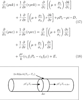
The following equations for turbulent energy (k) and the corresponding energy dissipation rate (") in cylindrical coordinates are simultaneously solved with Equations 1 to 3 to predict the velocity and tempera-ture proles in both radial and axial directions [23].
@
@z(uk) + 1 r
@
@r(rvk) = @ @z
+t
k
@k @z
+1r@r@
+t
k
r@k@r
+Pk " D;
(17) @
@z(u") + 1 r
@
@r(rv") = @ @z
+t
"
@" @z
+1r@r@
+t
"
r@"@r
+"k(c1f1Pk c2f2") + E; (18)
Figure 8. Schematic diagram of the heating, holding or cooling zone of a sterilization process.
where u and v represent the velocity components in z and r directions and the turbulent viscosity may be computed from the following equation [21]:
t= cfk 2
" : (19)
The entire set of partial dierential equations is simul-taneously solved via a control volume technique using conventional software. Figure 9 shows the ultimate grids for the entire CTS process, including heating, holding and cooling zones.
Figure 10a shows that for relatively large Reynolds numbers (Re 10000), the velocity prole of the heating zone is almost a piston type and the residence time can be computed with reasonable accuracy using an average velocity. Evidently, the Reynolds number increases due to a decrease in the uid viscosity, as the uid travels along the heating zone.
Figure 10b also shows various temperature pro-les for dierent sections of the heating zone (wall temperature = 403 K). As can be seen, the computed temperature distributions are nearly at and the radial dependency of the uid temperature may be ignored.
Figure 11 compares various bulk temperatures computed from the Nusselt method and the k " model for dierent heating zone wall temperatures. Although the Nusselt method slightly overestimates bulk temperatures initially, it does converge to the exact bulk temperatures computed via the k " model. Since the Dittus and Boetler equation employed in the Nusselt method is only valid for moderate temperature driving forces, the predicted heat transfer coecient error increases as the wall temperature of the heating zone rises.
A comparison of Figures 6 and 11 reveals that in contrast to the laminar ow, the bulk temperature of the uid in the turbulent ow reaches the heating zone wall temperature at 3 meters from the entrance. Hence,
Figure 9. GAMBIT generated mesh for the entire continuous thermal sterillization process.
Figure 10. Radial turbulent ow velocity and temperature distributions for heating zone.
Figure 11. Comparison of bulk temperature computed along the heating zone from Nusselt method and k " model.
for a xed length of heating zone, the accumulated lethality and the corresponding decrease in food quality will be very large for turbulent conditions. The holding zone length is usually very small for a turbulent ow and can be neglected in many situations.
Figure 12 clearly illustrates that the predicted accumulated sterility under turbulent conditions is
Figure 12. Comparison of sterility and quality
parameters for laminar and turbulent conditions in various heating zone wall temperatures.
several orders of magnitude greater than the similar situation in which laminar ow prevails. The maximum sterility value for a laminar condition with the highest wall temperature (180C) is around 500s after uid
passes the 24 meters of the heating and holding zone lengths. Note that the sterility of the food product at a similar temperature will be over one million seconds, which is about three orders of magnitude greater than the laminar condition. Surprisingly, the quality of the food products for all turbulent conditions is always lower than similar values computed for laminar ows. Therefore, using the turbulent condition drastically reduces the lengths of the heating and holding zones and, hence, signicantly preserves the quality of the food product.
The laminar temperature and velocity proles of Figure 12 are computed via the exact method (as shown previously), while the k " model is used for calculation of similar distributions under turbulent conditions.
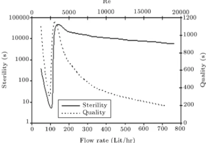
Figure 13 shows variations of sterility and quality parameters with a volumetric ow rate (or Reynolds number). Increasing the ow rate under laminar conditions initially decreases both sterility and quality parameters due to residence time reduction. However, as the uid enters the turbulent region, both
param-Figure 13. Variations of sterility and quality parameters with volumetric ow rate (heating zone wall temperature = 140C).
eters encounter a sharp increase. The sterility then slightly decreases as the volumetric ow rate increases, while the quality parameter severely decreases, as the Reynolds number increases, because of a major de-crease in residence time. Figure 13 demonstrates that an unpredicted transition from a laminar condition to a slightly turbulent situation should be avoided, since it can drastically reduce the quality of the food product. Simulation of CTS Process in the Presence of Suspended Solid Particles
To the best of our knowledge, the eect of solid particles in the simulation of CTS processes has not received sucient attention in previous articles. In many practical situations, the sterilized uid contains a considerable amount of small solid particles (such as fat, gelatin and starch), which can coagulate together and produce relatively large particles [24]. The spores or other pathological macroorganisms may be trapped in the center of such coagulated particles. Evidently, the amount of accumulated sterility will drop sharply for such entrapped spores (because of the solid particle heat resistance). Furthermore, these particles may undergo dierent trajectories in a turbulent ow. The eects of a particle trajectory and its heat transfer resistance on both quality and sterility parameters are considered in the following sections.
Solid Particles Trajectory in Turbulent Flow Suciently small particles often move along the streamlines of the laminar ow. Therefore, the surfaces of such particles are in thermal equilibrium with the corresponding streamlines. In turbulent ow, the movement of small particles is usually aected by the random movement of eddies. Furthermore, the tube wall can also reect the particle and produce a complex trajectory. Figure 14 demonstrates the
computed trajectory of a solid particle in a turbulent ow (Re 10000) inside a circular duct with a wall temperature of 140C. The corresponding calculations
were carried out, based on the random walk model using conventional software [25]. The geometry of the circular duct and the physical properties of the uid are presented in Table 1. Characteristics of the solid particle are also shown in Table 2.
It should be noted that the particle trajectory is only important when the temperature prole is not too at (piston type). In this case, the surface of the solid particle realizes various temperatures when passing through dierent points along the duct axis. Evidently, such a temperature history should be used to calculate both sterility and quality parameters. Fig-ure 15 illustrates three dierent temperatFig-ure proles for various Reynolds numbers at various sections of the heating zone. Although the temperature prole for a fully turbulent ow (Re = 10000) is completely at, the temperature distribution of a transition zone (Re = 3000) and laminar condition (Re = 2000) is far from being a piston type and the trajectory of the solid particle along the duct axis should be used to compute reliable values for both quality and sterility parameters. The transition zone prole was computed using the arithmetic average of the laminar and turbulent temperature distributions at Re = 3000. Solid Particles Thermal Resistance
The thermal resistances of solid particles have usually been ignored in many previous works and the solid particles are considered as lumped systems. Although this assumption may be valid for small particles,
Figure 14. Predicted trajectory of a solid particle in turbulent ow in a tube.
Table 2. Physical properties of the solid particle. Diameter
(m)
k (W/m.K)
Cp (kJ/kg.K)
Density (kg/m3)
various ow regimes.
distributed models are required to take account of the thermal resistance of relatively large solid particles. It is clear that the center temperature of such particles (d > 100 m) is much lower than their surface tem-peratures. Therefore, the lumped assumption yields to misleadingly large sterility values.
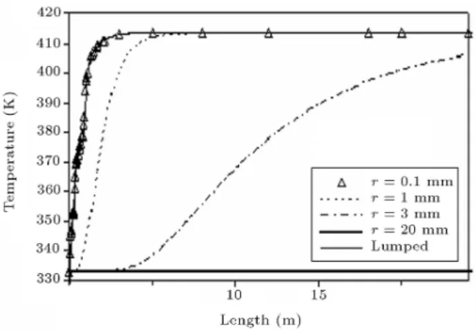
Figure 16 compares the distributed model pre-dictions of central temperatures for various sizes of solid particles with a corresponding lumped model. The wall temperature of the heating zone and the uid Reynolds number were considered as 140C and
10000, respectively. It is clearly shown that the central temperature of the large particles (d > 3 mm) is much lower than the surface temperature (lumped systems). A large number of food products contain suspended solids with various sizes between 3 to 20 millimeters [26].
The solid particle trajectory and the correspond-ing temperature history were computed rst via the conventional software. The central temperatures and the corresponding sterility values were then calculated using in-house software. Figure 17 emphasizes that the
Figure 16. Comparison of central temperatures computed via lumped and distributed models (Tw= 413 K).
Figure 17. Comparison of sterility values computed via lumped and distributed models (Tw= 413 K).
actual sterility received at the center of a large solid particle is much smaller than that predicted by the lumped assumption.
CONCLUSIONS
Simulations of CTS processes were considered for both laminar and turbulent conditions. It was clearly shown that for laminar ow, the nite dierence method performs adequately. It was also illustrated that simple heuristics of (Vmax Tbulk) and (Vaverage Tcenter)
provide the best predictions compared to the exact solution of the laminar situation. Furthermore, using a mixer at the entrance of the holding zone (while keeping other parameters constant) leads to a sharp increase in the sterility value, while decreasing the quality destruction.
A relatively simple empirical method, based on a dimensionless Nusselt number, was presented for turbulent conditions, and provided practically the same results compared to the more sophisticated method of the control volume technique. It was also illustrated that during laminar operations, great care should be taken to avoid entering the turbulent region. Such a condition drastically reduces the quality of the food product.
Using the turbulent condition also critically re-duces the length of both heating and holding zones and, hence, signicantly preserves the quality of the food product. The trajectories of solid particles in a transitionally turbulent ow are proved to be important and it was emphasized that the thermal resistances of relatively large solid particles should be also considered for the calculation of both sterility and quality parameters.
NOMENCLATURE C quality value (s)
C mean integrated quality value (s) at reference temperature
Cp; Cv uid specic heat; J/kgK
d pipe diameter; m
D decimal reduction time; s
DRef decimal reduction time (s) at reference
temperature F sterility value (s)
F mean integrated sterility value (s) at reference temperature
h(x) heat transfer coecient after x m of a pipe
k thermal conductivity; W/mK, turbulent energy; J/kg
_m uid mass ow rate; kgs 1
N number of microorganisms 1
N0 initial number of microorganism
Nf nal number of microorganism
P pressure; Pa
q heat ux; W/m2
_Q uid volumetric ow rate; m3s 1
r radial position in a pipe; m
R maximum pipe radius; m
t time; s
T temperature in Kelvin or Celsius vave uid average velocity within a section
of a pipe; m.s 1
v(r) uid velocity at the radial position (r) in a pipe; m.s 1
x axial position in a pipe; m
z temperature change (C) producing a
10-fold dierence in decimal reduction time
Greek Letters
dynamic viscosity; kg/ms t turbulent viscosity; kg/ms
density; kg/m3
" turbulent energy dissipation rate; m2/s
shear stress; Pa
Abbreviations
CTS Continuous Thermal Sterilization HTST High-Temperature-Short-Time UHT Ultra-High-Temperature REFERENCES
1. Manson, J.E. and Cullen, J.F. \Thermal process simulation for aseptic processing of foods containing
discrete particulate matter", Journal of Food Science, 39, p. 1084 (1974).
2. Saguy, I. and Karel, M. \Modeling of quality dete-rioration during food processing and storage", Food Technology, 34(2), pp. 78-85 (1980).
3. Snyder, G. \A mathematical model for prediction of temperature distribution in thermally processed shrimp", M.Sc. Thesis, University of Florida (1986). 4. Engelman, M. and Sani, R.L. \Finite element
simu-lation of an in-package pasteurization process", Num. Heat Transfer, 6(41), pp. 41-54 (1983).
5. Thorne, S. \Mathematical modeling of food processing operations", Elsevier Applied Science series (1992). 6. Zhang, L. and Fryer, P.J. \Models for the electrical
heating of solid liquid food mixtures", Chem. Engng. Sci., 48(4), pp. 633-642 (1993).
7. Wadad, G.Kh. and Sastry, S.K. \Eect of uid vis-cosity on the ohmic heating rate of solid-liquid mix-tures", Journal of Food Engineering, 27(2), pp. 145-158 (1996).
8. Baptista, P.N., Oliveria, F.A.R., Oliveria, J.C. and Sastry, S.K. \The eect of translational and rotational relative velocity components on uid-to-particle heat transfer coecients in continuous tube ow", Food Research International, 30(1), pp. 21-27 (1997). 9. Fryer, P.J. \Thermal treatment of foods", in Chemical
Engineering for the Food Industry, P.J. Fryer, D.L. Pyle and C.D. Rielly, Eds., London, Blackie A & P, pp. 331-382 (1977).
10. Holdsworth, S.D. \Aseptic processing and packaging of food products", Elsevier Applied Science, London (1992).
11. Jung, A. and Fryer, P.J. \Optimizing the quality of safe food: Computational modeling of a continuous sterilization process", Chemical Engineering Science, 54(6), pp. 717-730 (1999).
12. Sahoo, P.K., Ansari, I.A. and Datta, A.K. \Computer aided design and performance evaluation of an indirect type helical tube ultra-high temperature (UHT) milk sterilizer", J. Food Eng., 51, pp. 13-19 (2002). 13. Zhong, Q., Sandeep, K.P. and Swartzel, K.R.
\Contin-uous ow radio frequency heating of particulate foods", Innovative Food Science and Emerging Technologies, 5, pp. 475-483 (2004).
14. Salengke, S. and Sastry, S.K. \Experimental investi-gation of ohmic heating of solid-liquid mixtures under worst-case heating scenarios", Journal of Food Engi-neering, 83, pp. 324-336 (2007).
15. Salengke, S. and Sastry, S.K. \Models for ohmic heat-ing of solid-liquid mixtures under worst-case heatheat-ing scenarios", Journal of Food Engineering, 83, pp. 337-355 (2007).
16. Launder, B.E. and Spalding, D.B., Lectures in Mathe-matical Models of Turbulence, Academic Press, London (1972).
Selected Applications, Academic Press, London (1979). 23. Dang, C. and Hihara, E. \In-tube cooling heat transfer
food sterilizer design", Chemical Engineering Science, 52(12), pp. 1835-1843 (1977).

![Figure 4. Comparison of computed temperature distributions with reported values of Jung and Fryer [9].](https://thumb-us.123doks.com/thumbv2/123dok_us/8399052.2231585/4.892.464.809.844.1012/figure-comparison-computed-temperature-distributions-reported-values-fryer.webp)