ISSN: 2322-1666 print/2251-8436 online
ONE-STAGE UNCERTAIN LINEAR OPTIMIZATION
ZEINAB ZAREA AND ALIREZA GHAFFARI-HADIGHEH
Abstract. Uncertainty is one of the intrinsic features of natural phe-nomenon and optimization is not an exception. Parameters in an op-timization problem may be inaccurately presented, or due to variation after solving the problem, the current optimal solution may not be optimal or feasible for the new data. One of the approaches towards the uncertainty is the uncertainty theory initiated by Liu in 2007 and completed in 2011. This theory describes the uncertainty orig-inated from human reasoning in mathematical axiomatic words. In this paper, we consider one-stage uncertain linear optimization prob-lem, where the parameters linearly depend on several independent uncertain variables. A solution method is presented which is similar to the branch and bound method for the integer linear program. The presented methodology is explained by simple illustrative examples.
Key Words: Uncertainty Theory, One-stage uncertain optimization problem, Linear Opti-mization.
2010 Mathematics Subject Classification:Primary: 90C05; Secondary: 68T37.
1. Introduction
Linear Optimization (LO) has been studied from different points of view and has proved its ability in modeling a vast range of practical problem in various fields. It is numerically tractable its theory is almost complete and powerful solvers have been developed. One of the basic assumptions in an LO problem is certainty of the parameters while this is not always the case in practice. In some cases, parameters are not estimated exactly
Received: 15 January 2018, Accepted: 21 January 2018. Communicated by A. Youse-fian Darani;
∗Address correspondence to A. Ghaffari-Hadigheh; E-mail: [email protected] c
2018 University of Mohaghegh Ardabili. 36
and sometimes they are changed after solving the problem. Consequently the obtained optimal solution may not be optimal or feasible more.
Let us consider an LO problem as (1.1) min
x { n
X
j=1
cjxj : n
X
j=1
aijxj ≤bi, i= 1, . . . , m, xj ≥0, j= 1, . . . , n}.
Using sensitivity analysis and parametric programming is a traditional approach and there are many published results with different points of views (See e.g. [5, 4, 12]). In sensitivity analysis, the effect of substitu-tion of a parameter with another value is investigated. If this parameter is in the objective function, the optimality may be affected. While the change in the right-hand-side data may result the current optimal solu-tion being infeasible. When this substitusolu-tion occurs in the right-hand-side of constraints, the current optimal solution might be neither feasible nor optimum. Additionally, the goal of parametric programming is finding a region for parameters, where a specific feature of the problem is invariant. For instance, it may be the interval where the optimal basis is invariant whenc1varies. When variation occurs in the right hand side of constraints,
the optimal solution may be change while the optimal basis is the same. Observe that in sensitivity analysis and parametric programming, new value of parameters is still considered exact values.
Another point of view to handle the indeterminacy is Fuzzy Theory [10]. Here, parameters of the problem are considered as fuzzy numbers and eventually a crisp linear program is produced and solved [9]. The main weak point of fuzzy models is that, the fuzzy number used in the model is not known and applying different fuzzy numbers may result in different and sometimes contradictory results.
Robust optimization could be another approach for managing uncer-tainty. In this method, it is assumed that data belongs to a set but with-out any specific probability distribution [6]. For example, the objective function coefficient vector might be in an ellipsoid. The vector is close to the border as the same possibility as it could be next to the centroid. A special case is the interval LO problem [8]. In this case, each parameter varies independently in an interval, while in general they might be bound to each other in some way. In the interval LO, for example, objective function coefficient vector is in a hyper-rectangular instead of an ellipsoid. We must note that the intervals themselves are identified by an expert and they are fixed afterward. Thus, a sort of uncertainty still affects the problem. In the robust LO problem, the model reduces to a crisp one to
produce an optimal solution such that for all parameters in these intervals, it is still optimal, while the notion of optimality is somehow different.
One may want to address the uncertainty using probability theory. In such an approach, a probability distribution is associated with each un-certain parameter. For example, c1 might have a uniform distribution
and thus its expected value can be considered instead. One of the main deficiencies of this approach is that, for exact estimation of appropriate probability distribution, enough number of historical data is necessary. Moreover, the obtained optimal solution is not the desired one in practice and it could be only a kind of assurance during a decision making process. In stochastic linear programming, uncertainty may appear in satisfying of constraints, and a lower bound for the probability of the satisfaction could be considered [2]. For example, instead of a linear constraint in (1.1), the following is replaced.
gi(x) =P( n
X
j=1
aijxj ≤bi)≥αi,
where 0 ≤ αi ≤ 1 and is selected by the decision maker. Observe that
gi(x) =P(Pnj=1aijxj ≤bi) is nonlinear in general and even it is not
con-vex in some cases. This will add a higher rate complexity to the problem. In an LO problem, when there is no enough credible data to estimate the probability distribution of the underlying indeterminate data or the problem violates the fuzzy rules, one may have no choice but relying on the human reasoning. Uncertainty theory has been initiated in 2007 [6] and then refined in 2011 [7] is an axiomatic paradigm to answer the uncertainty originated from the expert’s opinion.
An uncertain problem can be defined as one-stage or multi-stage prob-lem. In a one-stage uncertain problem, all decisions are made in one step, while in multi-stage uncertain problems, some decisions must be made be-fore any realization of the uncertain phenomenon. Some other decisions are taken after the realization of the uncertain phenomenon stage by stage. LO in an uncertain environment has been investigated in [3]. The author proposed two different models and all input data are considered as inde-pendent uncertain variables. The results also were demonstrated on sim-ple examsim-ples. Two-stage uncertain linear optimization has been studied in [11]. The authors considered this problem in several cases and proposed a solution approach. In this paper, we consider one-stage uncertain LO problem. It is assumed that, in addition to some crisp constraints, there are some other uncertain constraints. These later constraints are linearly
dependent on several uncertain variables. The uncertain variables are all considered to be linear since the methodology is independent of the type of uncertain variable. We also assume that the belief that an uncertain con-straint holds with minimum belief rate prescribed by the decision maker. The methodology for solving such problems is represented and illustrated using some concrete examples.
This paper is organized as follows. In Section 2, basic concepts of uncertainty theory are reviewed. The one-stage uncertain LO problem is presented in Section 3. A computational algorithm is devised in Section 4. Final Section includes some concluding remarks.
2. Uncertainty Theory
Let us review some basic prerequisite concepts of the uncertainty theory. Let Γ be a nonempty set, and L consists of subsets of Γ be a σ-algebra over Γ. The pair (Γ, L) is called a measurable space, and each member Λ∈L of this measurable space is called an event. An uncertain measure is a functionM from L to [0,1] which satisfies the following axioms.
• (Normality Axiom) For the universal set Γ,M{Γ}= 1. • (Duality Axiom)M{Λ}+M{Λc}= 1 for any event Λ.
• (Subadditivity Axiom) M{
∞
[
i=1
Λi} ≤
∞
X
i=1
M{Λi} for all countable
sequence of events Λ1,Λ2, . . .
The value of M{Λ} indicates the belief degree to the event “We believe Λ will happen”. The triplet (Γ, L, M) is called an uncertainty space. Liu in [6] has defined an additional axiom to the uncertain measure which distinguishes the uncertainty theory from the probability theory.
• (Product Axiom) Let (Γk, Lk, Mk), k = 1,2, . . . be uncertainty
spaces. The product uncertain measureM is an uncertain measure satisfying
M{
∞
Y
k=1
Λk}=
∞
^
k=1
Mk{Λk},
Where Λk is an event in Γk and k= 1,2, . . ..
A function f : (Γ, L) → R is measurable if for any Borel set B in R,
the inverse image of f is a member of the σ -Algebra L. This means that f−1(B) = {γ :f(γ) ∈B} ∈L. All continuous functions and mono-tone functions are measurable functions. An uncertain variable ξ is a
measurable function from (Γ, L, M) to R. For an uncertain variable, the
uncertainty distribution Φ is defined by Φ(x) =M{ξ≤x}.
There are several uncertainty distributions in the literature. Since our results are independent of the distribution type, we only remind the linear uncertain distribution and refer to [6] for the others.
A linear uncertain distribution is denoted by L(a, b) and defined as
Φ(x) =
0 if x≤a x−a
b−a if a≤x≤b 1 if x > b.
wherea < bare two real numbers. A regular uncertainty distribution Φ(x) is a continuous and strictly increasing function that satisfy 0<Φ(x)<1 , limx→−∞Φ(x) = 0, and limx→+∞Φ(x) = 1. For a regular uncertainty
distribution Φ(x) on(0,1), well-defined inverse function Φ−1(α) exits and is called the inverse uncertainty distribution of ξ. Inverse uncertainty distribution of the linear variableL(a, b) is Φ−1(α) = (1−α)a+αb.
Uncertain variables ξ1, ξ2, . . . , ξn are called independent if and only if
for arbitrary Borel setsB1, B2, . . . , Bn, it holds
M{
n
\
i=1
ξi ∈Bi}=
^
i=1,...,n
M{ξi∈Bi}.
An uncertain variable ξ is nonnegative when M{ξ < 0} = 0, and it is positive when M{ξ ≥0} = 1. Analogous definitions can be provided for nonpositive and negative uncertain variables.
Theorem 2.1. [6]Let ξ1, ξ2, . . . , ξn be uncertain variables. Further, let f be a measurable real-valued function. Then f(ξ1, ξ2, . . . , ξn) be an uncer-tain variable.
Observe that there is no direct way to compute the value of a function that depends on an uncertain variable, specially when it appears in a constraint. One useful alternative in to apply the α-chance counterpart. In this situation, satisfying such constraint is replaced by a minimum belief degree that an uncertain constraint holds. Such a constraint then can be easily calculated using the inverse uncertainty distribution as stated in the following theorem.
Theorem 2.2. [6] Let ξ1, ξ2, . . . , ξn be independent uncertain variables with regular uncertainty distributions Φ1,Φ2, . . . ,Φn, respectively. Con-sider the function ξ = f(ξ1, ξ2, . . . , ξn) is strictly increasing with respect
toξ1, ξ2, . . . , ξm, m≤n, and strictly decreasing with respect toξm, . . . , ξn. Then M{f(ξ1, ξ2, . . . , ξn)≤0} ≥α, if and only if
f(Φ1−1(α),Φ−21(α), . . . ,Φ−m1(α),Φm−1+1(1−α), . . . ,Φ−n1(1−α))≤0. 3. One-Stage Uncertain Linear optimization
A one-stage uncertain LO can be defined in a general form as (3.1) min{cTx|T(ξ)x≥h(ξ), x∈X},
whereξ: Ω→Rr is an uncertain vector on the uncertain space (Γ, L, M).
Here, T(ξ) is an uncertain matrix of m×n dimension and h(ξ) ∈ Rs is
an uncertain vector depending on the uncertain vector ξ. In general, it is assumed thatT(ξ), h(ξ) is independent of the decision variable x. This means that our decision does not affect uncertain input data. Let
(3.2) ζ(x, ξ) :=T(ξ)x−h(ξ). Further, let
(3.3) T(ξ) =T +
r
X
j=1
Tjξj, h(ξ) =h+ r
X
j=1
hjξj.
Eq. (3.3) can be rewritten asζi(x, ξ) :=tTi (ξ)x−hi(ξ), i= 1, . . . , m, where
tT
i is the i-th row ofT(ξ). Therefore
(3.4)
ζi(x, ξ) := tTi x−hi+ r
X
j=1
tTijξjx− r
X
j=1
hijξj
=
n
X
k=1
tikxk−hi+ r
X
j=1
ξj( n
X
k=1
tijkxk−hij).
Using the simplifying notations ¯
di = n
X
k=1
tikxk−hi and dij = n
X
k=1
tijkxk−hij,
we have
(3.5) ζi(x, ξ) := ¯di+ r
X
j=1
ξjdij.
The α-chance form of problem (3.1) is
Using (3.5), constraints of Problem (3.6) is converted to the following form.
(3.7) M{
r
X
j=1
ξj(−dij)≤d¯i} ≥α, i= 1, . . . , m.
Let us define v+ =
0, v <0 v, v≥0 and v
− =
−v, v≤0
0, v >0 . Based on Theorem
2.2, Eq. (3.7) holds if and only if (3.8)
r
X
j=1
(−dij)+Φ−j1(α)− r
X
j=1
(−dij)−Φ−j1(1−α)≤d¯i, i= 1, . . . , m.
Considering these facts, Problem (3.1) is simplified as a crisp LO prob-lem
(3.9) min{c
Tx| r
X
j=1
(−dij)+Φ−j1(α)−
r
X
j=1
(−dij)−Φ−j1(1−α)≤d¯i,
i= 1, . . . , m, x∈X}. In the sequel, we solve Problem (3.9), step by step. First, we consider that the problem only has one uncertain constraint, i.e.,i= 1.
3.1. Case r= 1. We first consider that the problem depends on only one uncertain variable,ξ = (ξ1). Therefore, Problem (3.9) is specialized as
(3.10) min{cTx|M{(−d1)ξ1≤d} ≥¯ α, x∈X}.
Recall that x varies in X, and consequently d1 might be positive
(non-negative) of negative, depending on the vector x. We consider then two subcases.
(1) Letd1≥0. We first add this constraint to the problem. Moreover,
(−d1)+= 0,(−d1)−=d1. Therefore, M{(−d1)ξ1 ≤d} ≥¯ α if and
only if −(d1)Φ−1(1−α) ≤d. Considering the uncertain variable¯ as a linear as ξ1 =L(a, b), we have the following equivalent crisp
constraint
(3.11) −d1(b+ (a−b)α)≤d¯
Therefore, Problem (3.9) is reduced to
(2) Let d1 ≤ 0. We add this constraint to the problem. Further,
(−d1)+ = −d1,(−d1)− = 0. Then, M{(−d1)ξ1 ≤d} ≥¯ α, if and
only if−(d1)Φ−1(α)≤d. With the assumption that the uncertain¯
variable is linear asξ1 =L(a, b),we have the following equivalent
crisp constraint.
(3.13) −d1(a+ (b−a)α)≤d.¯
Therefore, the problem (3.7) is replaced with the following prob-lem.
(3.14) min{cTx| −d1(a+ (b−a)α)≤d, d¯ 1≤0, x∈X}.
Solving two problems (3.12) and (3.14) for a given belief rate α may result to several outcomes. If both problems are infeasible, then the prob-lem has no solution for the given α. Reducing the value of belief degreeα may result to a feasible and consequently optimal solution. If at least one of these problems has finite optimal solution, then the one-stage uncertain LO has an optimal solution as well. If both problems have optimal solu-tion, then the optimal solution of the one-stage uncertain LO is obtained with one of the Problems (3.12) and (3.14).
Let us explain the methodology with a simple example.
Example 3.1. Consider the following problem. In this problem, we con-sidered α= 0.9.
(3.15)
min −2x1−x2
s.t. M{(3x1−x2+ 2)ξ1 ≤2x2−3} ≥0.9
x1+x2 ≤3
x1≥0, x2≥0,
whereξ1=L(1,3).Here,−d1= 3x1−x2+ 2 and ¯d= 2x2−3. Considering
d1≥0, the following LO problem produces.
(3.16)
min −2x1−x2
s.t. 3x1−x2+ 2≤0
3.6x1−3.2x2 ≤ −5.4
x1+x2 ≤3
x1 ≥0, x2 ≥0.
An optimal solution of this problem is (x1, x2) = (0.25,2.75) and the
If d1 ≤0, we have the following LO problem.
(3.17)
min −2x1−x2
s.t. 3x1−x2+ 2≥0
8.4x1−4.8x2≤ −8.6
x1+x2≤3
x1≥0, x2 ≥0.
An optimal solution of Problem (3.17) is (x1, x2) = (0.439,2.561), with
the objective valuez=−3.439. Comparison of Problems (3.16) and (3.17) reveals that the optimal solution of the one-stage uncertain LO problem (3.15) is (x1, x2) = (0.439,2.561).
3.2. Case r = 2. In this case, we suppose that the input data depends on two independent uncertain variables ξ1 and ξ2. We still assume that
the problem has a single uncertain constraint. Corresponding problem is (3.18) min{cTx|M{ξ1(−d1) +ξ2(−d2)≤d} ≥¯ α, x∈X}.
Depending on the values ofd1andd2(both varies withx) four subproblem
are identified.
(1) Let ∈ X is such that d1 ≥ 0 and d2 ≥ 0. We will add these
inequities to the problem. Moreover
(3.19) M{−ξ1(−d1)−−ξ2(−d2)−≤d} ≥¯ α,
holds if and only if
(3.20) −d1Φ−11(1−α) +d2Φ−21(1−α)≤d.¯
With the assumption ξ1 = L(a1, b1) and ξ2 = L(a2, b2), (21) is identical
with
(3.21) −d1(b1+ (a1−b1)α)−d2(b2+ (a2−b2)α)≤d.¯
Therefore, Problem (3.18) reduces to (3.22)
min{cTx| −d
1(b1+ (a1−b1)α)−d2(b2+ (a2−b2)α)≤d,¯
d1 ≥0, d2 ≥0, x∈X}.
Without further details, crisp LO problems in other three cases are as follows.
(1) With the assumption d1 ≤0 and d2 ≥ 0 , we have the following
problem. (3.23)
min{cTx| −d
1(a1+ (b1−a1)α)−d2(b2+ (a2−b2)α)≤d,¯
d1 ≤0, d2 ≥0, x∈X.}
(2) With the assumption d1 ≥0 and d2 ≤ 0 , we have the following
problem. (3.24)
min{cTx| −d
1(b1+ (a1−b1)α)−d2(a2+ (b2−a2)α)≤d,¯
d1≥0, d2≤0, x∈X}.
(3) With the assumption d1 ≤0 and d2 ≤ 0 , we have the following
problem. (3.25)
min{cTx| −d
1(a1+ (b1−a1)α)−d2(a2+ (b2−a2)α)≤d,¯
d1≥0, d2≤0, x∈X}.
Solving these problems produces the optimal solution of the Prob-lem (3.18). If none of the Problems (3.22)-(3.25) is feasible, the Problem (3.18) has no solution for the belief rateα. Feasible solution may be pos-sible with smaller values ofα. When some of these problems has optimal solution, then the solution of (3.18) is identical with the one with smallest objective value. Let us explain the result via a simple example.
Example 3.2. Consider the following one-stage uncertain LO problem. In all subproblems, we fixed the belief rate atα= 0.9.
(3.26)
min −2x1−x2
s.t. M{(x1−x2)ξ1+ (−2x1+x2−2)ξ2≤2x2−3} ≥0.9
x1+x2 ≤3
x1≥0, x2 ≥0,
whereξ1 =L(1,3) andξ2 =L(2,4). In the first three cases, the problems
have optimal solutions as follows, while the optimization problem in the final case is infeasible. The objective values and optimal solutions are as follows.
(1) (x1, x2) = (1.5,1.5) andz=−4.5.
(2) (x1, x2) = (0.333,2.667) andz=−3.333.
(3) (x1, x2) = (3,0) and z=−6.
Therefore, for the belief rate α = 0.9, optimal solution of problem (3.26) is produced by the third case as (x1, x2) = (3,0) and z=−6.
As these two cases reveal, when there is only a single uncertain con-straint withrindependent uncertain variables, the solution approach leads to 2rsubproblems, with possible infeasibility of some. In the next section, we present and algorithm for finding the solution when more than one uncertain constraint exists.
4. Computational Algorithm
Let us organize the solution approach as an algorithm. The suggested algorithm runs like the branch and bound algorithm in the integer LO problem. To explain the algorithm, we restrict it to the case r= 2, with multiple uncertain constraints. It can be easily generalized for arbitrary number of uncertain variables. We also assume that the two uncertain variables are linear asξ1 =L(a1, b1) and ξ2 = L(a2, b2). In this way, we
have the following uncertain problem. (4.1)
min{cTx|M{−ξ
1(−d1i)−ξ2(−d2i)≤d¯i} ≥α, i= 1, . . . , m, x∈X}.
Starting Step. Solve the problem ignoring uncertain constraints. If this problem is infeasible,Stop. The uncertain problem (4.1) has no solution for any belief rateα.
Branching Step. (1) Seti= 1.
(2) Depending on the values of d1i and d2i, consider 4 subproblems.
To each subproblem, three additional constraints are added to the problem in the parent node.
(3) Solve each produced problem.
(4) If one of these subproblems is infeasible, cut the branching of that node at the subsequent branching step.
(5) Save all existing optimal solutions and objective values.
(6) Ifi=m, go to the next tep, otherwise set i:=i+ 1, and go to 2. Decision Making Step
(1) If there is no saved optimal solution and object value, Stop. The problem (4.1) has no solution.
(2) Find the smallest objective value. The optimal solution of the corresponding subproblem is the optimal solution of (4.1).
For more details let us mention one of the subproblems as (4.2) min{c
Tx| −d
11(b1+ (a1−b1)α)−d21(b2+ (a2−b2)α)≤d¯1,
First Level Constraints Node Name Second Level Constraints Optimal Solution Objective Value d11≥0, d12≥0
C11 d21≥0, d22≥0 x= (0,0) z= 0
C12 d21≥0, d22≤0 x= (0.32,0.32) z=−0.32
C13 d21≤0, d22≥0 Infeasible N.A.
C14 d21≤0, d22≤0 Infeasible N.A.
d11≥0, d12≤0
C21 d21≥0, d22≥0 Infeasible N.A.
C22 d21≥0, d22≤0 Infeasible N.A.
C23 d21≤0, d22≥0 Infeasible N.A.
C24 d21≤0, d22≤0 Infeasible N.A.
d11≤0, d12≥0
C31 d21≥0, d22≥0 x= (1,0) z=−2
C32 d21≥0, d22≤0 x= (0.75,0.25) z=−1.75
C33 d21≤0, d22≥0 x= (3,0) z=−6
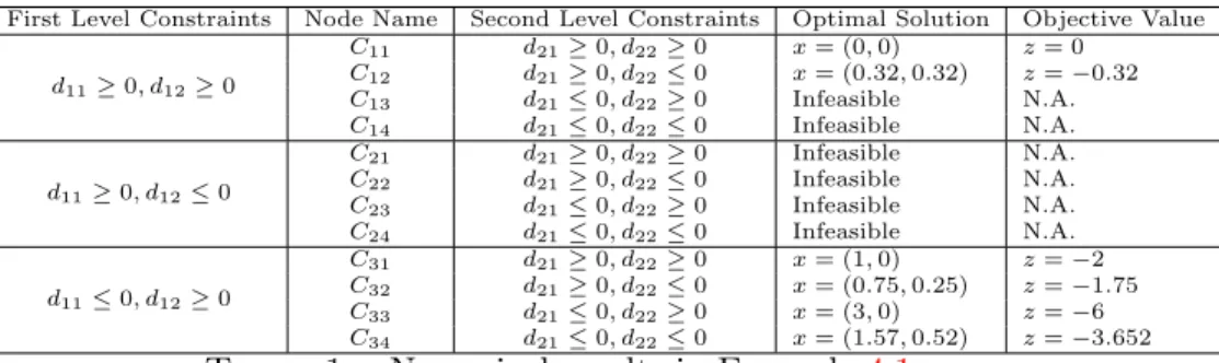
C34 d21≤0, d22≤0 x= (1.57,0.52) z=−3.652 Table 1. Numerical results in Example 4.1.
and in a sample subproblem to the problem (4.2) in level i = 2 , the following three constraints will be added.
(4.3) −d11(b1+ (a1−b1)α)−d21(b2+ (a2−b2)α)≤d¯1, d11≥0, d21≥0,
We assert that when the uncertain problem (4.1), has no feasible solution, the decision maker may desire to reduce the value of belief rate to have a feasible and consequently an optimal solution.
To illustrate the algorithm, we continue with two simple examples.
Example 4.1. Consider the following problem. We fixed the belief rate at α= 0.9.
(4.4)
min −2x1+x2
s.t. M{(x1−x2)ξ1+ (−2x1+x2−2)ξ2≤2x2−3} ≥0.9
M{(x1+x2−1)ξ1+ (−x1+ 3x2)ξ2 ≤x1−x2+ 2} ≥0.9
x1+x2 ≤3, x1 ≥0, x2 ≥0
where ξ1 =L(1,3) and ξ2 =L(2,4). The results are depicted in Table 1.
Here, optimization problem in some nodes are infeasible, specially when at the first leveld11≤0, d12≤0, which is dropped from the table. As the
results reveal, an optimal solution of (4.4) is (x1, x2) = (3,0), with the
First Level Constraints Node Name Second Level Constraints Optimal Solution Objective Value d11≥0, d12≥0
C11 d21≥0, d22≥0 x= (−1,0) z= 1
C12 d21≥0, d22≤0 x= (0,−2) z=−6
C13 d21≤0, d22≥0 x= (−1,0) z= 1
C14 d21≤0, d22≤0 x= (−1,0) z= 1
d11≥0, d12≤0
C21 d21≥0, d22≥0 x= (−1,0) z= 1
C22 d21≥0, d22≤0 x= (−0.7,0.1) z= 1
C23 d21≤0, d22≥0 x= (−1.118,0.236) z= 1.829
C24 d21≤0, d22≤0 x= (−1.092,0.184) z= 1.642
d11≤0, d12≥0
C31 d21≥0, d22≥0 x= (0,−2) z=−6
C32 d21≥0, d22≤0 x= (3.69,−9.379) z=−31.82
C33 d21≤0, d22≥0 x= (0,0.333) z= 1
C34 d21≤0, d22≤0 x= (0,0.333) z= 1
d11≤0, d12≤0
C41 d21≥0, d22≥0 x= (0,0.333) z= 1
C42 d21≥0, d22≤0 x= (0,0.247) z= 0.74
C43 d21≤0, d22≥0 x= (0,0.396) z= 1.188
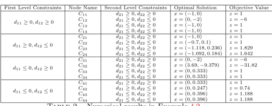
C44 d21≤0, d22≤0 x= (0,0.396) z= 1.188 Table 2. Numerical results in Example4.2.
Example 4.2. Consider the following problem. We fixed the belief rate at α= 0.95.
(4.5)
min −x1+ 3x2
s.t. M{2x1ξ1+ (−x1+ 3x2−1)ξ2≤x1+x2} ≥0.95
M{(−x1+ 2x2−2)ξ1+ (2x1+x2+ 3)ξ2≤3x1−2x2+ 3} ≥0.95
x1+x2≤3
whereξ1 =L(2,4) and ξ2 =L(1,2).The results are depicted in Table 2.
As the results show, all subproblems have optimal solution, and an optimal solution of (4.5) is (x1, x2) = (3.69,−9.379), with the objective value
z=−31.82, identified by the subproblem in Node C32.
5. Concluding Remarks
In this paper, we considered a one-stage LO problem, where some of its constraints data is uncertain and satisfying these constraints are desired with a prescribed belief rate. A computation algorithm was presented and the methodology is examined on some simple examples. Though the com-plexity of the algorithm was not studied, obviously it can be improved in the implementation by effective computational codes. For example, saving the final basis of a subproblem in each node can reduce the complexity of solving the subsequent subproblems. Moreover, using the depth-first
strategy in visiting the nodes could further reduce the computational ef-forts. The methodology can be generalized for other optimization prob-lems other than LO. One may also consider a bounding strategy in the pruning of the branches.
References
[1] A. Ben-Tal and A. Nemirovski, Robust solutions of linear programming problems contaminated with uncertain data, Mathematical programming,88(2000), 411-424. [2] J.R. Birge and F. Louveaux,Introduction to stochastic programming, Springer
Sci-ence & Business Media,(2011).
[3] A. Ghaffari-Hadigheh, Two linear programming models in uncertain environment (in Persian), Journal of Operational Research in Its Applications,50, 37-51. [4] A. Ghaffari-Hadigheh and N. Mehanfar,Matrix Perturbation and Optimal Partition
Invariancy in Linear Optimization, Asia-Pacific Journal of Operational Research,
32(2015).
[5] A. Ghaffari-Hadigheh and Terlaky Tams, Sensitivity analysis in linear optimiza-tion: Invariant support set intervals, European Journal of Operational Research,
169(2006), 1158-1175.
[6] B. Liu,Uncertainty theory, Springer, (2007).
[7] B. Liu,Uncertainty theory: A branch of mathematics for modeling human uncer-tainty, Springer,300(2011).
[8] G.H. Huang and M.F. Cao,Analysis of Solution Methods for Interval Linear Pro-gramming, Journal of Environmental Informatics,17(2011).
[9] H. Naseri,Fuzzy Simplex Methods for Fuzzy uncertain linear programming, Oper-ations Research and ApplicOper-ations,4(2013).
[10] H. Tanaka and K. Asai, Fuzzy linear programming problems with fuzzy numbers, Fuzzy Sets and Systems,13(1984),1-10.
[11] M. Zheng, Y. Yi, Z. Wang and J.F. Chen,Study on two-stage uncertain program-ming based on uncertainty theory, Journal of Intelligent Manufacturing, (2017), 633-642.
[12] Roos, Cornelis, Terlaky, Tams and Vial,Interior point algorithms for linear opti-mization, Springer Science, (2005).
Zeinab Zarea
Department of Applied Mathematics, Azarbaijan Shahid Madani University Tabriz, Iran
Email: zareh [email protected]
Alireza Ghaffari-Hadigheh
Department of Applied Mathematics, Azarbaijan Shahid Madani University Tabriz, Iran