PJM Renewable Integration Study

(1)

GE

Energy Consulting

PJM Renewable

Integration Study

Executive Summary Report

Revision 03

Prepared for: PJM Interconnection, LLC.

Prepared by: General Electric International, Inc.

(2)

PJM Renewable Integration Study Legal Notices

Legal Notices

This report was prepared by General Electric International, Inc. (GE) as an account of work sponsored by PJM Interconnection, LLC. (PJM). Neither PJM nor GE, nor any person acting on behalf of either:

1. Makes any warranty or representation, expressed or implied, with respect to the use of any information contained in this report, or that the use of any information, apparatus, method, or process disclosed in the report may not infringe privately owned rights.

2. Assumes any liabilities with respect to the use of or for damage resulting from the use of any information, apparatus, method, or process disclosed in this report.

(3)

PJM Renewable Integration Study Contact Information

Contact Information

This report was prepared by General Electric International, Inc. (GEII); acting through its Energy Consulting group (GE) based in Schenectady, NY, and submitted to PJM Interconnection, LLC. (PJM). Technical and commercial questions and any correspondence concerning this document should be referred to:

Gene Hinkle

Manager, Investment Analysis GE Energy Management Energy Consulting 1 River Road Building 53 Schenectady, NY 12345 USA Phone: (518) 385 5447 Fax: (518) 385 5703 [email protected]

(4)

PJM Renewable Integration Study Table of Contents

List of Figures

Figure 1: PJM Wind and Solar Capacity by State for 14% RPS Scenario ... 5

Figure 2: Duration Curves of PJM Load and Load-Net-Renewables for Study Scenarios ... 10

Figure 3: Ten-Minute Wind and Solar Variability as Function of Production Level for Increasing Renewable Penetration ... 11

Figure 4: Average Daily Wind Profile by Season for 14% RPS and 30% LOBO Scenarios ... 12

Figure 5: Smoothing of Plant-Level 10-Minute Variability over PJM’s Footprint, June 14, 30% LOBO ... 13

Figure 6: Ten-Minute Variability in Wind and Solar Output as a Function of Production Level ... 15

Figure 7: Sample Day Showing 10-Minute Periods that Exceeded Ramp Capability ... 16

Figure 8: Annual Energy Production by Unit Type for Study Scenarios ... 20

Figure 9: PJM Annual Operation Trends for Study Scenarios ... 23

Figure 10: Trends in Production Costs and Transmission Costs versus Renewable Penetration ... 24

Figure 11: CT Capacity Committed (2% BAU, July 28) ... 27

Figure 12: Demand MW, Renewable Dispatch, and # of CTs Committed in RT (30% LOBO, February 17) ... 27

Figure 13: LMP Comparison for Several 20% and 30% Scenarios (March 4) ... 28

Figure 14: Effective Load Carrying Capability of a Resource ... 29

Figure 15: Types of Cycling Duty That Affect Cycling Costs ... 31

Figure 16: Net Effect on Cycling Damage Compared to 2% BAU Scenario ... 32

Figure 17: Impact of Cycling Effects on Total Production Costs for 2% BAU and 30% LOBO Scenarios ... 33

Figure 18: SOx Emissions for Study Scenarios, With and Without Cycling Effects Included ... 35

Figure 19: NOx Emissions for Study Scenarios, With and Without Cycling Effects Included... 35

Figure 20: Sensitivity Analysis Results for 20% LOBO Scenario; Total Emissions and Energy by Unit Type ... 39

Figure 21: Process for Calculating Real-Time Regulation Requirements ... 43

Figure 22: Production Cost Reduction with 4-Hour-Ahead Recommitment, 14% RPS Scenario ... 45

Figure 23: CT Dispatch for Existing Day-Ahead Unit Commitment Practice and 4-Hour-Ahead Recommitment (14% RPS Scenario, May 26) ... 45

(6)

PJM Renewable Integration Study List of Tables

List of Tables

Table 1: Total PJM Wind and Solar Capacity for Study Scenarios ... 4

Table 2: Forecasted Fuel Prices for Study Year 2026 ... 6

Table 3: Estimated Regulation Requirements for Study Scenarios ... 15

Table 4: Ten-minute Periods Exceeding Ramp Capability for Selected Scenarios ... 16

Table 5: New Lines and Transmission Upgrades for Study Scenarios ... 18

Table 6: Annual Production Cost and Energy Displacement by Unit Type for Study Scenarios ... 21

Table 7: Renewable Contribution to Lowering Production Cost ... 25

Table 8: Range of Effective Load Carrying Capability (ELCC) for Wind and Solar Resources in 20% and 30% Scenarios ... 30

Table 9: Variable O&M Costs ($/MWh) Due to Cycling Duty for Study Scenarios... 32

Table 10: CO2 Emissions from PJM Power Plants for Study Scenarios ... 36

Table 11: Sensitivity Analysis Results for 2% BAU Scenario ... 37

Table 12: Sensitivity Analysis Results for 14% RPS Scenario ... 37

Table 13: Sensitivity Analysis Results for 20% LOBO Scenario ... 38

Table 14: Sensitivity Analysis Results for 30% LOBO Scenario ... 38

(7)

PJM Renewable Integration Study Project Overview

1 Project Overview

At the request of its stakeholders, PJM Interconnection, LLC. (PJM) initiated this study to perform a comprehensive impact assessment of increased penetrations of wind and solar generation resources on the operation of the PJM grid. The principal objectives include:

• Determine, for the PJM balancing area, the operational, planning, and energy market effects of large-scale integration of wind and solar power as well as mitigation/facilitation measures available to PJM

• Make recommendations for the implementation of such mitigation/facilitation measures

This study is motivated by the need for PJM to be prepared for a considerably higher penetration of renewable energy in the next 10 to 15 years. Every jurisdiction within the PJM footprint, except for Kentucky and Tennessee, has a renewable portfolio standard (RPS), or Alternative Energy Portfolio Standard (AEPS), or non-binding Renewable Portfolio Goal (RPG)1_.

This study investigates operational, planning, and energy market effects of large-scale wind/solar integration, and makes recommendations for possible facilitation/mitigation measures. It is not a detailed near-term planning study for any specific issue or mitigation. The target year is 2026, which was used to estimate the PJM annual load profile used in the study scenarios.

The growth of renewable energy is largely driven by Renewable Portfolio Standards and other legislative policies. The cost-benefit economics of renewable resources, and quantifying the capital investment required to install additional wind and solar infrastructure, were beyond the scope of this study and were not investigated. The study assumed that the penetration of renewable resources would increase and investigated how the PJM system would be affected.

The impact of renewables on production cost savings was investigated, but the analysis did not include possible secondary impacts to the capacity market such as increased retirements due to non-economic performance or a possible need for generators to recover more in the capacity market because of reduced revenue in the energy market.

Project Team

Six companies joined forces to execute the broad range of technical analysis required for this study.

(8)

PJM Renewable Integration Study Project Overview

• GE Energy Consulting – overall project leadership, production cost and capacity value analysis

• AWS Truepower – development of wind and solar power profile data

• EnerNex – statistical analysis of wind and solar power, reserve requirement analysis • Exeter Associates – review of industry practice/experience with integration of

wind/solar resources

• Intertek Asset Integrity Management (Intertek AIM), formerly APTECH – impacts of increased cycling on thermal plant O&M costs and emissions

• PowerGEM – transmission expansion analysis, simulation of sub-hourly operations and real-time market performance

Data Sources

This study used a combination of publicly available and confidential data to model the Eastern Interconnection, the PJM grid, and its power plants. In order to protect the proprietary interests of PJM stakeholders, the production simulation analysis was primarily based on publically available data, reviewed and vetted by PJM to assure consistency with the operating characteristics of the PJM grid and the power plants under its control. The sub-hourly analysis used PowerGEM’s Portfolio Ownership and Bid Evaluation (PROBE) program, which is regularly used by PJM to monitor the performance of the real-time market2_{. PROBE uses proprietary power plant data, but that data was not shared with any}

other study team members per PJMs existing non-disclosure agreement with PowerGEM. AWST provided wind and solar power generation profiles and power forecasts within the PJM interconnection region, as well as the rest of the Eastern Interconnection, as inputs to hourly and sub-hourly grid simulations. These data sets were based on high-resolution simulations of the historical climate performed by a mesoscale numerical weather prediction (NWP) model covering the period 2004 to 2006.

Meteorological data from NREL’s EWITS project3_{was used to produce power output profiles}

for both wind and solar renewable energy generation facilities. A site selection process was completed for onshore and offshore wind as well as for the centralized and distributed solar sites within the PJM region. The selection includes sites that could be developed to meet and exceed renewable portfolio standards for the PJM Interconnection. Power output profiles were produced for each of the sites using performance characteristics from the most

2_{PowerGEM website,}_{http://www.power-gem.com/PROBE.htm} 3_{http://www.nrel.gov/docs/fy11osti/47078.pdf}

(9)

PJM Renewable Integration Study Study Scenarios

current power conversion technologies as of July 2011. The resulting wind and solar power profiles were validated against measurements.

2 Study Scenarios

Table 1 summarizes the PJM wind and solar installed capacity for the ten study scenarios. Note that the scenarios are defined in terms of percentage of renewable energy generation (MWh), whereas Table 1 summarizes the wind and solar capacity (MW) in each scenario. Also, all scenarios include 1.5% of non-wind, non-solar renewable generation.

2% BAU: This is a Business As Usual (BAU) reference case with the existing level of wind/solar in year 2011. This case is a benchmark for how PJM operations will change as wind and solar penetration increases.

14% RPS: Wind and solar generation meets existing RPS mandates by 2026, with

14% renewable energy penetration in PJM.

20% LOBO: 20% wind and solar energy penetration in PJM, Low Offshore and Best

Onshore; 10% of wind resources are offshore, 90% of wind resources are onshore in locations with best wind quality.

20% LODO: 20% wind and solar energy penetration in PJM, Low Offshore and Dispersed Onshore; 10% of wind resources are offshore, 90% of wind resources are onshore. Incremental onshore wind added in proportion to load energy of individual states.

20% HOBO: 20% wind and solar energy penetration in PJM, High Offshore and Best Onshore; 50% of wind resources are offshore, 50% of wind resources are onshore in locations with best wind quality.

20% HSBO: 20% wind and solar energy penetration in PJM, High Solar and Best Onshore; similar to 20% LOBO, but with twice the solar energy and proportionately less wind energy.

The 30% scenarios are similar to the 20% scenarios, but with more wind and solar resources to achieve 30% wind and solar energy penetration in PJM.

(10)

PJM Renewable Integration Study Study Scenarios

Table 1: Total PJM Wind and Solar Capacity for Study Scenarios Scenario Renewable Penetration in PJM Onshore Wind (MW) Offshore Wind (MW) Centralized Solar (MW) Distributed Solar (MW) Total (MW) 2% BAU 2% 5,122 0 72 0 5,194 14% RPS 14% 28,834 4,000 3,254 4,102 40,190 20% LOBO 20% 39,452 4,851 8,078 10,111 62,492 20% LODO 20% 40,942 4,851 8,078 10,111 63,982 20% HOBO 20% 21,632 22,581 8,078 10,111 62,402 20% HSBO 20% 32,228 4,026 16,198 20,294 72,746 30% LOBO 30% 59,866 6,846 18,190 16,907 101,809 30% LODO 30% 63,321 6,846 18,190 16,907 105,264 30% HOBO 30% 33,805 34,489 18,190 16,907 103,391 30% HSBO 30% 47,127 5,430 27,270 33,823 113,650

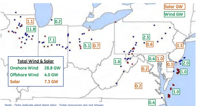
Figure 1 shows the locations of wind plants for the 14% RPS scenario. Note the high concentration of wind plants in Illinois, Indiana and Ohio, which have high quality wind resources. Other study scenarios where onshore wind resources were selected based on a “best sites” criteria also have high concentrations of wind plants in these western PJM states. Scenarios with the “dispersed sites” criteria moved some of the Illinois and Indiana wind resources eastward, to Ohio, Pennsylvania, and West Virginia.

(11)

PJM Renewable Integration Study Study Assumptions

Figure 1: PJM Wind and Solar Capacity by State for 14% RPS Scenario

Most of the scenario technical analysis was performed using wind, solar and load profiles from year 2006. Four scenarios (2% BAU, 14% RPS, 20% LOBO, and 30% LOBO) were analyzed with 2004, 2005, and 2006 renewable and load profiles, in order to quantify differences in performance using different profile years. Although there were some observable differences in operational and economic performance due to differences in wind and solar production across the three profile years, the overall impacts were relatively small and did not affect the study conclusions.

3 Study Assumptions

PJM annual load energy was extrapolated to the study year 2026 using a method to retain critical daily and seasonal load shape characteristics. The average annual load growth for PJM was assumed to be 1.1%4_{. Load for the rest of the Eastern Interconnection was based}

on Ventyx “Historical and Forecast Demand by Zone”.

New thermal generators (about 35 GW of SCGT and 6 GW of CCGT) were added to the PJM system in the 2% BAU scenario to meet the reserve margin requirements in 2026 consistent

4_{The base case assumed a PJM net energy forecast of 969,596 GWh in 2026 (excluding EKPC) based on the 2011 PJM Load}

Forecast Report (January 2011). The 2014 Preliminary PJM Load Forecast report shows a net energy forecast of 889,841 GWh in 2026 excluding EKPC, i.e., a reduction of 8.2%.

1.0 11.8 7.1 0.4 1.6 5.1 2.0 0.2 0.4 1.0 2.5 Wind GW Solar GW 0.2 0.2 0.6 0.7 3.3 1.0 1.1 0.3

Total Wind & Solar

Onshore Wind 28.8 GW Offshore Wind 4.0 GW

Solar 7.3 GW

(12)

PJM Renewable Integration Study Major Conclusions and Recommendations

with the assumed load growth (for a total of about 65 GW of SCGT and 38 GW of CCGT). For consistency across scenarios, the new thermal generators added to meet reserve requirements in the 2% BAU scenario remained available in all higher renewable penetration scenarios. The additions included ISA/FSA qualified plants from the PJM queue, but rest of the additions were not reflective of other future projects in the PJM queue.

Some existing PJM power plants were assumed to retire by 2026, per retirement forecast data from PJM and Ventyx.

All operating power plants were assumed to have the necessary control technologies to be compliant with emissions requirements. No emission or carbon costs were assumed in the base scenarios although Carbon costs were considered in one of the sensitivity cases.

Fuel prices used for production cost simulations are shown in Table 2.

Table 2: Forecasted Fuel Prices for Study Year 2026

Fuel Type Nominal Price Source Comments

Natural Gas $8.02/MMBtu EIA 2012 Energy _Outlook At Henry Hub; Regional basis differentials _{provided by PJM} Coal $3.51/MMBtu EIA 2012 Energy _Outlook _{($1.15 to $6.08) per Ventyx historical usage data}Adjusted to reflect regional price differences Nuclear $0.75/MMBtu _{Velocity Forecast}Ventyx Energy

Residual No.2 Oil $15.04/MMBtu _{NYMEX Forecast}Energy Velocity Adjusted to include monthly variation patterns _{($14.92 to $15.20)} LS No.2 Diesel $22.56/MMBtu _{NYMEX Forecast}Energy Velocity Adjusted to include monthly variation patterns _{($22.37 to $22.79)}

The wind profiles produced for this study used performance characteristics from the most current power conversion technologies as of July 2011. Therefore, the power output profiles are slightly higher than what has been historically observed in PJM.

4 Major Conclusions and Recommendations

A brief summary of the major conclusions and recommendations are listed here. Further details are presented in subsequent sections of this report.

Conclusions

The study findings indicate that the PJM system, with adequate transmission expansion and additional regulating reserves, will not have any significant issues operating with up to 30%

(13)

of its energy provided by wind and solar generation. The amount of additional transmission5

and reserves required are briefly defined later in this summary and in much greater detail in the main body of the report.

• Although the values varied based on total penetration and the type of renewable generation added, on average, 36% of the delivered renewable energy displaced PJM coal fired generation, 39% displaced PJM gas fired generation, and the rest displaced PJM imports (or increased exports).

• No insurmountable operating issues were uncovered over the many simulated scenarios of system-wide hourly operation and this was supported by hundreds of hours of sub-hourly operation using actual PJM ramping capability.

• There was minimal curtailment of the renewable generation and this tended to result from localized congestion rather than broader system constraints.

• Every scenario examined resulted in lower PJM fuel and variable Operations and Maintenance (O&M) costs as well as lower average Locational Marginal Prices (LMPs). The lower LMPs, when combined with the reduced capacity factors, resulted in lower gross and net revenues for the conventional generation resources. No examination was made to see if this might result in some of the less viable generation advancing their retirement dates.

• Additional regulation were required to compensate for the increased variability introduced by the renewable generation. The 30% scenarios, which added over 100,000 MW of renewable capacity, required an annual average of only 1,000 to 1,500 MW of additional regulation compared to the roughly 1,200 MW of regulation modeled for load alone. No additional operating (spinning) reserves were required. • In addition to the reduced capacity factors on the thermal generation, some of the

higher penetration scenarios showed new patterns of usage. High penetrations of solar generation significantly reduced the net loads during the day and resulted in economic operation which required the peaking turbines to run for a few hours prior to sun up and after sun set rather than committing larger intermediate and base load generation to run throughout the day.

• The renewable generation increased the amount of cycling (start up, shut down and ramping) on the existing fleet of generators, which imply increased variable O&M costs on these units. These increased costs were small relative to the value of the fuel displacement and did not significantly affect the overall economic impact of the renewable generation.

5_{This study did not examine the cost allocation for the transmission expansion required to deliver the renewable energy in}

(14)

• While cycling operations will increase a unit’s emissions relative to steady state operations, these increases were small relative to the reductions due to the displacement of the fossil fueled generation.

Recommendations

Adjustments to Regulation Requirements

The amount of regulation required by the PJM system is highly dependent upon the amount of wind and solar production at that time. It is recommended that PJM develop a method to determine regulation requirements based on forecasted levels of wind and solar production. Day-ahead and shorter term forecasts could be used for this purpose.

Renewable Energy Capacity Valuation

Capacity value of renewable energy has a slightly diminishing return at progressively higher penetration, and the LOLE/ELCC approach provides a rigorous methodology for accurate capacity valuation of renewable energy.

PJM may want to consider an annual or bi-annual application of methodology in order to calibrate its renewable capacity valuation methodology in order to occasionally adjust the applicable capacity valuation of different classes of renewable energy resources in PJM. Mid-Term Commitment & Better Wind and Solar Forecast

Inherent errors in the day-ahead forecasts for wind and solar production lead to suboptimal commitment of generation resources in real-time operations, especially if simple cycle combustion turbines are the primary resources used to compensate for any generation shortages. Wind and solar forecasts are much more accurate in the four- to five-hour-ahead timeframe than in the current day-five-hour-ahead commitment process. It is recommended that PJM consider using such a mid-range forecast in real-time operations to update the commitment of intermediate units (such as combined cycle units that could start in a few hours). The wind and solar forecast feature can be added to the current PJM application called Intermediate Term Security Constrained Economic Dispatch (IT SCED)6_{which is used to}

commit CT’s and guides the Real Time SCED (RT SCED) by looking ahead up to two hours. This would result in less reliance on higher cost peaking generation.

Exploring Improvements to Ramp Rate Performance

Ramp-rate limits on the existing baseload generation fleet may constrain PJM’s ability to respond to rapid changes in net system load in some operating conditions. It is

6_{"Real-time Security-Constrained Economic Dispatch and Commitment in the PJM: Experiences and Challenges", Simon}

(15)

PJM Renewable Integration Study Statistical Characteristics of Load, Wind and Solar Profiles

recommended that PJM explore the reasons for ramping constraints on specific units, determine whether the limitation are technical, contractual, or otherwise, and investigate possible methods for improving ramp rate performance.

5 Statistical Characteristics of Load, Wind and

Solar Profiles

A wide variety of statistical evaluations were performed on the load, wind and solar profiles to build understanding on how they would impact the annual, seasonal, daily, and short-term operation of the PJM grid. A few examples are presented here.

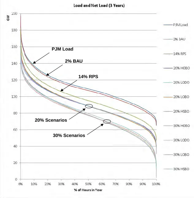
Figure 2 exhibits duration curves of load-net-renewables (wind + solar), which show the portion of the PJM load that must be served by non-renewable generation resources. The right-hand portions of the curves show that in the higher penetration scenarios, renewables serve about half of total system load during low-load periods.

(16)

Figure 2: Duration Curves of PJM Load and Load-Net-Renewables for Study Scenarios

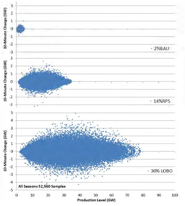
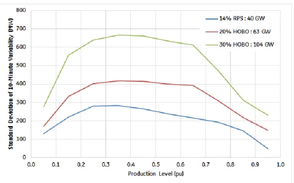
Figure 3 shows 10-minute variability (i.e., the change in 10-minute renewable production from one 10-minute period to the next) as a function of total renewable production for three scenarios with increasing renewable penetration (2%, 14%, and 30%). One significant trend is that the maximum 10-minute variations occur when renewable production is about half of total renewable capacity. Variability is lower near maximum production levels, partly because many wind plants are operating above the knee in the wind-power curve where changes in wind speed do not affect electrical power output. This characteristic of variability is relevant to the regulation requirements, which is discussed later.

PJM Load 2% BAU

14% RPS

20% Scenarios

(17)

Figure 3: Ten-Minute Wind and Solar Variability as Function of Production Level for Increasing Renewable Penetration

Figure 4 shows average daily wind profiles by season for two scenarios. The trends show lower power output during the midday hours, especially during the summer season. This trend is complementary to solar profiles which naturally peak during midday and have higher production during the summer season.

(18)

Figure 4: Average Daily Wind Profile by Season for 14% RPS and 30% LOBO Scenarios

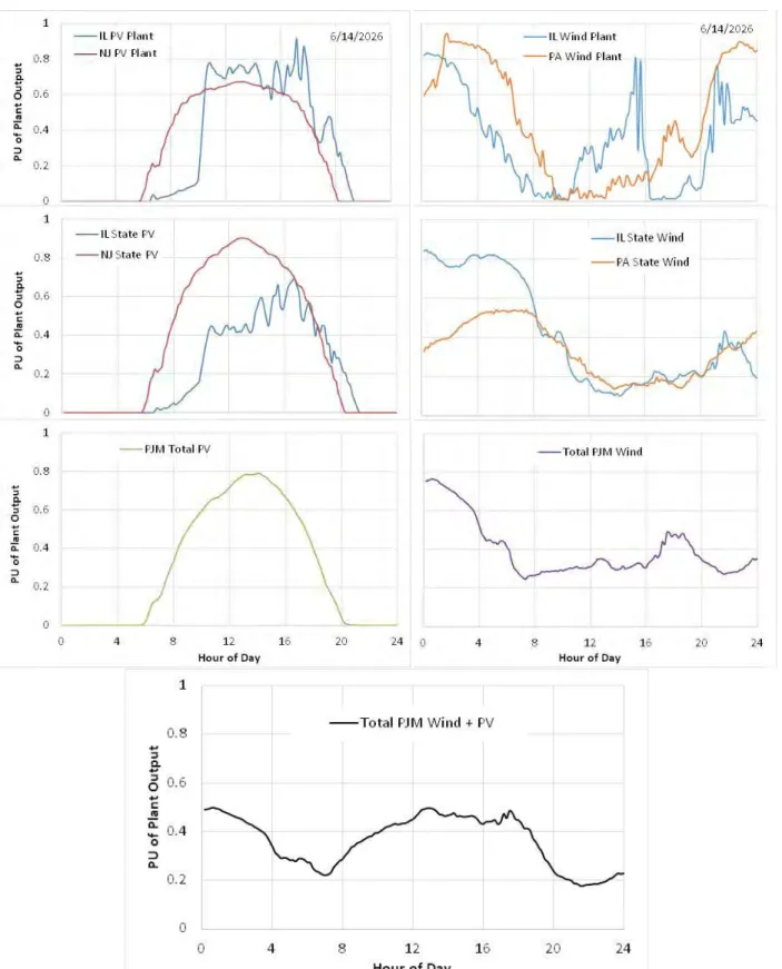
Figure 5 illustrates how the variability of individual wind and solar PV plants is reduced when all wind and solar PV plants are aggregated over PJM’s footprint. The upper traces show the high variability associated with individual plants. The two wind plants and the Illinois solar plant show high short term variability. The New Jersey solar plant has a smooth profile, indicating a relatively clear or hazy day. The next traces below show the aggregate profiles for all wind and solar plants within the states of New Jersey, Pennsylvania, and Illinois. The lower traces show profiles for all wind plants in PJM, all PV plants in PJM, and the combination of all wind and PV plants in PJM. Short-term variability is dramatically reduced when aggregated across PJM’s footprint. Values shown are in terms of per units of capacity ratings. PJM’s large geographic footprint is of significant benefit for integrating wind and solar generation, and greatly reduces the magnitude of variability-related challenges as compared to smaller balancing areas.

14% RPS Scenario

(19)

(20)

PJM Renewable Integration Study Regulation and Reserves

6 Regulation and Reserves

With increasing levels of wind and solar generation, it will be necessary for PJM to carry higher levels of reserves to respond to the inherent variability and uncertainty in the output of those resources. Currently PJM has four categories of ancillary services:

• Regulation, which include generating units or demand response resources that are under automatic control and respond to frequency deviations,

• Reserves, which include Contingency (Primary) Reserve (combination of Synchronized and Non-Synchronized Reserves), and Secondary Reserve,

• Black Start Service, which include generating units that can start and synchronize to the system without having an outside (system) source of AC power, and

• Reactive Services, which help maintain transmission voltages within acceptable limits.

Statistical analysis of wind, PV and load data was employed to determine how much additional regulation capacity would be required to manage renewable variability in each of the study scenarios. The regulation requirement for wind and solar was combined with the regulation requirement for load (a percentage of peak or valley load MW, per PJM rules) to calculate a total regulation requirement.

The analysis illustrated that the variability of wind and solar power output is a function of the total production level (see Figure 6). More regulation are needed when production is at mid-level, and less regulating reserves are needed when production is very low or very high. Previous studies have established that a statistically high level of confidence for reserve is achieved at about 3 standard deviations (or 3σ in industry parlance) of 10-minute renewable variability. The 3σ criterion was also adopted for this study, which means that the regulation requirements are designed to cover 99.7% of all 10-minute variations. Table 3 summarizes the range of regulation required for each scenario. In the production cost and sub-hourly simulations, the amount of regulation was adjusted hourly as a function of the total renewable energy production in each hour.

(21)

Figure 6: Ten-Minute Variability in Wind and Solar Output as a Function of Production Level

Table 3: Estimated Regulation Requirements for Study Scenarios

Regulation Load Only 2% BAU 14% RPS 20% HOBO 20% LOBO 20% LODO 20% HSBO 30% HOBO 30% LOBO 30% LODO 30% HSBO Maximum (MW) 2,003 2,018 2,351 2,507 2,721 2,591 2,984 3,044 3,552 3,191 4,111 Minimum (MW) 745 766 919 966 1,031 1,052 976 1,188 1,103 1,299 1,069 Average (MW) 1,204 1,222 1,566 1,715 1,894 1,784 1,958 2,169 2,504 2,286 2,737 % Increase Compared to Load 1.5% 30.1% 42.4% 57.3% 48.2% 62.6% 80.2% 108.0% 89.8% 127.4%

From a contingency perspective, none of the wind or solar plants added to the PJM system was large enough such that their loss would increase PJM’s present level of contingency reserves. And given the large PJM footprint for a single balancing area, the impacts of short-term variability in wind and solar production is greatly reduced by aggregation and

geographic diversity.

The following approach was adopted to assess the need for additional ancillary services due to wind and solar variability:

• Simulate hourly operation using GE MAPS, with regulation allocated per the criteria described above and contingency reserves per PJM’s present practices.

• Using the hourly results of the GE MAPS simulations, compare the ramping capability of the committed units each hour with the sub-hourly variability of wind and solar production in that hour.

(22)

• Quantify the number of periods where ramping capability is insufficient.

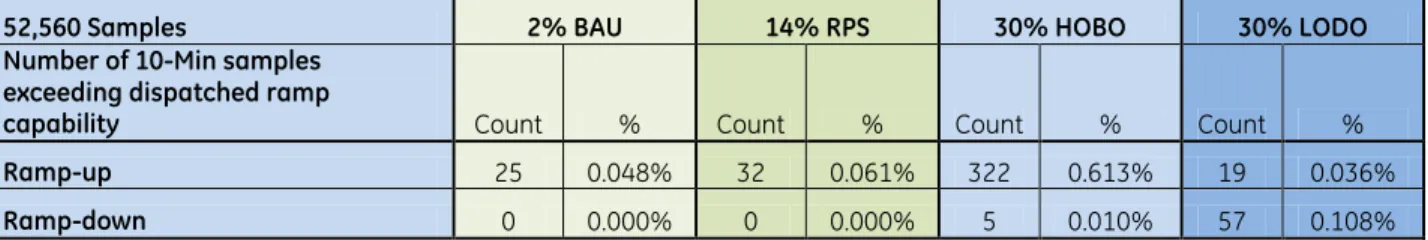
Figure 7 is an excerpt from the ramp analysis, showing a day with three 10-minute periods when the change in net load (red dots) exceed the ramp-up capability of the committed generators (green line). Table 4 summarizes the analytical results for several scenarios, and shows that there are relatively few periods in a year when renewable ramps exceed fleet ramping capability, and those few events would not likely cause an unacceptable decrease in PJM’s Control Performance Standard (CPS) measures.

The adequacy of the regulation was further confirmed by the challenging days simulated in the PROBE sub-hourly analysis. The selection criteria specifically included days with low ramp-rate and ramp-range capability relative to wind and solar ramps.

The results of the combined analytical methods indicate that no additional operating reserves would be required for the study scenarios.

Figure 7: Sample Day Showing 10-Minute Periods that Exceeded Ramp Capability

Table 4: Ten-minute Periods Exceeding Ramp Capability for Selected Scenarios

52,560 Samples 2% BAU 14% RPS 30% HOBO 30% LODO

Number of 10-Min samples exceeding dispatched ramp

capability Count % Count % Count % Count %

Ramp-up 25 0.048% 32 0.061% 322 0.613% 19 0.036%

(23)

PJM Renewable Integration Study Transmission System Upgrades

7 Transmission System Upgrades

The transmission model was built upon the 2016 and 2017 Regional Transmission Expansion Plan (RTEP) models provided by PJM. New lines and other transmission upgrades were added to the transmission models for each study scenario to serve the increased load and generation resources. Given that the output of wind and solar resources inherently varies by time of day and season of year, the traditional transmission expansion planning methods were augmented by production cost analysis to ensure adequate transmission capacity without overbuilding. Some wind plants and thermal plants share common transmission corridors, and since wind plants are not dispatchable, it is not appropriate to size those corridors to accommodate simultaneous maximum output from both wind and thermal plants.

The transmission expansion process involved the following steps:

• Security-constrained optimal power flow analysis to identify transmission paths that are overloaded under contingency conditions and cannot be relieved by adjusting the dispatch.

• Generator deliverability analysis with wind and solar plant loaded to 100% of capacity value, to identify reliability problems that required transmission upgrades. • Generator deliverability analysis with wind and solar plant loaded to 100% of energy

value, to identify flowgates that could be overloaded and therefore should be monitored in production cost analysis.

• Production cost analysis to quantify annual transmission path utilization and congestion, and to identify paths with excessive congestion.

These steps were performed iteratively on each scenario to design a set of transmission upgrades that would achieve deliverability and reliability objectives while limiting congestion to a reasonable level. This was achieved by increasing transmission capacity until the largest contribution to congestion costs by a constrained element between two nodes with highest and lowest average annual LMP in the system was $5/MWh, averaged across the year.

Table 5 summarizes the transmission additions and upgrades for each scenario. New lines indicate new line construction on new or existing right-of-ways. Upgrades involve improvements to existing lines (i.e., reconductoring to increase current rating).

(24)

PJM Renewable Integration Study Impact of Renewables on Annual PJM Operations

Table 5: New Lines and Transmission Upgrades for Study Scenarios

8 Impact of Renewables on Annual PJM Operations

Hourly annual operation for all study scenarios was simulated using the GE Multi-Area Production Simulation (GE MAPS) model. GE MAPS model employs Security-Constrained Unit Commitment (SCUC) and Security-Constrained Economic Dispatch (SCED) to emulate the hourly operation of a competitive market and models the full transmission system to account for congestion. The results show the following impacts of higher wind and solar energy penetration on the PJM grid:

• Lower Coal and CCGT generation under all scenarios. Wind and solar resources are effectively price-takers and therefore displace more expensive generation resources. • Lower emissions of criteria pollutants and greenhouse gases, due to reduced

operation of thermal generation resources.

• No unserved load and minimal renewable energy curtailment. New thermal resources were added to meet reserve requirements for the 2% BAU case in 2026, and those resources were kept available for all higher renewable penetration Scenario 765 kV New Lines (Miles) 765 kV Upgrades (Miles) 500 kV New Lines (Miles) 500 kV Upgrades (Miles) 345 kV New Lines (Miles) 345 kV Upgrades (Miles) 230 kV New Lines (Miles) 230 kV Upgrades (Miles) Total (Miles) Total Cost (Billion) Total Congestion Cost (Billion) 2% BAU 0 0 0 0 0 0 0 0 0 $0 $1.9 14% RPS 260 0 42 61 352 35 0 4 754 $3.7 $4.0 20% Low Offshore Best Onshore 260 0 42 61 416 122 0 4 905 $4.1 $4.0 20% Low Offshore Dispersed Onshore 260 0 42 61 373 35 0 49 820 $3.8 $4.9 20% High Offshore Best Onshore 260 0 112 61 363 122 17 4 939 $4.4 $4.3 20% High Solar Best Onshore 260 0 42 61 365 122 0 4 854 $3.9 $3.3 30% Low Offshore Best Onshore 1800 0 42 61 796 129 44 74 2946 $13.7 $5.2 30% Low Offshore Dispersed Onshore 430 0 42 61 384 166 44 55 1182 $5.0 $6.3 30% High Offshore Best Onshore 1220 0 223 105 424 35 14 29 2050 $10.9 $5.3 30% High Solar Best Onshore 1090 0 42 61 386 122 4 4 1709 $8 $5.6

(25)

scenarios. This is a contributing factor in the result that in all scenarios there were adequate reserves and no instances of unserved load7_{. There were no operating}

conditions where wind/solar variability or uncertainty caused an insufficiency of generation. Nearly all of the wind and solar energy was used to serve load.

• Lower system-wide production costs (i.e., fuel and O&M costs for thermal generators) • Lower gross revenues for conventional generation resources

• Lower average LMP and zonal prices across the PJM grid

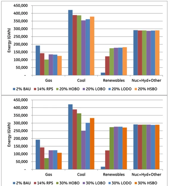
Figure 8 illustrates how the energy dispatch shifts from gas and coal generation to renewable resources as the renewable penetration increases. The upper plot shows the progression to 20% penetration and the lower plot extends to 30% penetration of wind and solar energy. On average for all scenarios, about 36% of the renewable energy displaces coal-based generation about 39% displaces gas-fired generation, as compared to the 2% BAU Scenario.

7_{If the study plan had assumed constant installed reserve margins across all study scenarios, there would likely have been}

(26)

Figure 8: Annual Energy Production by Unit Type for Study Scenarios

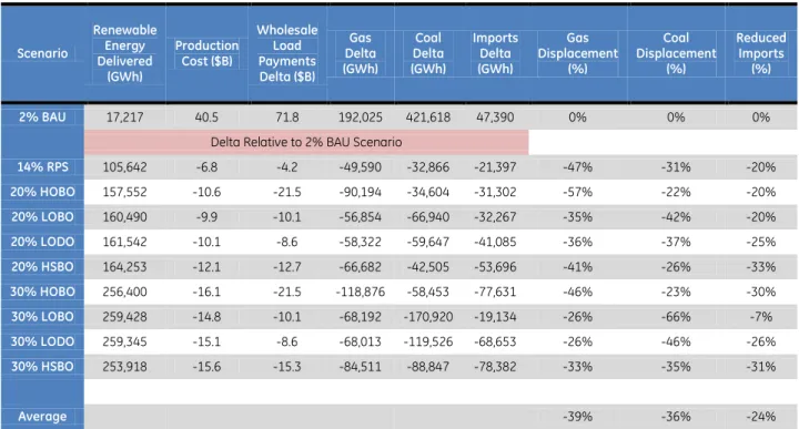
Table 6 shows how several economic and energy parameters are affected by increased renewables in the study scenarios. Changes are measured relative to the 2% BAU scenario. In the 14% RPS scenario, 47% of the additional renewable energy displaces gas-fired resources and 31% displaces coal. In several of the 20% and 30% scenarios, proportionately more coal energy is displaced.

50,000 100,000 150,000 200,000 250,000 300,000 350,000 400,000 450,000

Gas Coal Renewables Nuc+Hyd+Other

Ene

rgy

(GWh)

2% BAU 14% RPS 20% HOBO 20% LOBO 20% LODO 20% HSBO

50,000 100,000 150,000 200,000 250,000 300,000 350,000 400,000 450,000

Gas Coal Renewables Nuc+Hyd+Other

Ene

rgy

(GWh)

(27)

Table 6: Annual Production Cost and Energy Displacement by Unit Type for Study Scenarios

Scenario Renewable Energy Delivered (GWh) Production Cost ($B) Wholesale Load Payments Delta ($B) Gas Delta (GWh) Coal Delta (GWh) Imports Delta (GWh) Gas Displacement (%) Coal Displacement (%) Reduced Imports (%) 2% BAU 17,217 40.5 71.8 192,025 421,618 47,390 0% 0% 0%

Delta Relative to 2% BAU Scenario

14% RPS 105,642 -6.8 -4.2 -49,590 -32,866 -21,397 -47% -31% -20% 20% HOBO 157,552 -10.6 -21.5 -90,194 -34,604 -31,302 -57% -22% -20% 20% LOBO 160,490 -9.9 -10.1 -56,854 -66,940 -32,267 -35% -42% -20% 20% LODO 161,542 -10.1 -8.6 -58,322 -59,647 -41,085 -36% -37% -25% 20% HSBO 164,253 -12.1 -12.7 -66,682 -42,505 -53,696 -41% -26% -33% 30% HOBO 256,400 -16.1 -21.5 -118,876 -58,453 -77,631 -46% -23% -30% 30% LOBO 259,428 -14.8 -10.1 -68,192 -170,920 -19,134 -26% -66% -7% 30% LODO 259,345 -15.1 -8.6 -68,013 -119,526 -68,653 -26% -46% -26% 30% HSBO 253,918 -15.6 -15.3 -84,511 -88,847 -78,382 -33% -35% -31% Average -39% -36% -24%

Production Cost is sum of Fuel Costs, Variable O&M Costs, any Emission Tax/Allowance Costs, and Start-Up Costs – adjusted by adding Imports Costs and subtracting Export Sales. Coal, Gas, and Import Displacement values are the ratio of GWh reductions in each energy resource (Coal, Gas, Imports) relative to the GWh increase in Total Renewable Energy Delivered.

This study did not evaluate potential impacts on the PJM Capacity Market due to reduced generator revenues from the wholesale energy market, nor did it evaluate the impact of renewables on rate payers. It is conceivable that lower energy prices would be at least partially offset by higher capacity prices.

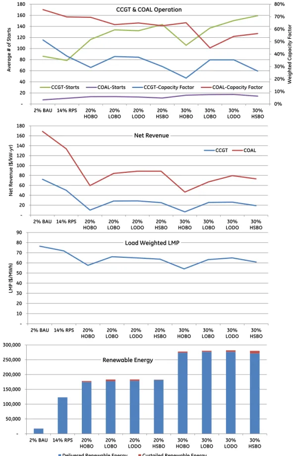
Figure 9 shows several annual operational trends for the study scenarios. Compared to the 2% BAU scenario,

• Coal and CCGT capacity factors decline with increasing renewables

• CCGT annual starts remain the same for the 14% RPS scenario and double for many of the 20% and 30% scenarios, indicating an increase in cycling duty. Annual starts for coal plants increase slightly, indicating that there are periods of the year when some coal plants are not committed.

• Net energy revenues for CCGT and coal plants decline significantly with increasing renewables, potentially leading to additional generator retirements. This study did

(28)

not look at revenue adequacy, potential retirements, or the cost to maintain resource adequacy.

• Most of the new renewable energy is used to serve load and only a small portion must be curtailed in the 20% and 30% scenarios, mostly due to local congestion.

(29)

Figure 9: PJM Annual Operation Trends for Study Scenarios

0% 10% 20% 30% 40% 50% 60% 70% 80% 20 40 60 80 100 120 140 160 180 2% BAU 14% RPS 20%

HOBO LOBO20% LODO20% HSBO20% HOBO30% LOBO30% LODO30% HSBO30%

W ei ghted Cap acity F acto r Av era ge # o f Star ts

CCGT & COAL Operation

CCGT-Starts COAL-Starts CCGT-Capacity Factor COAL-Capacity Factor

20 40 60 80 100 120 140 160 180 2% BAU 14% RPS 20% HOBO 20% LOBO 20% LODO 20% HSBO 30% HOBO 30% LOBO 30% LODO 30% HSBO Net Rev en ue ( $/kW -y r) Net Revenue CCGT COAL 10 20 30 40 50 60 70 80 90 2% BAU 14% RPS 20%

LM P ($/ M W h) Load Weighted LMP 50,000 100,000 150,000 200,000 250,000 300,000 2% BAU 14% RPS 20%

Ene

rgy

(GWh)

Renewable Energy

(30)

Figure 10 shows trends in total PJM production costs and transmission expansion/upgrade costs as a function of renewable penetration level. Production costs are fairly similar for all scenarios with the same renewable energy penetration. Estimated transmission costs are similar for all 20% penetration scenarios but dramatically different for the 30% scenarios. The 30% LOBO scenario includes a high concentration of wind power in the western PJM region, and significant transmission upgrades are needed to transport that wind energy to load centers. In the LODO scenario, wind resources are more dispersed across the PJM footprint, so the wind plants are closer to load centers.

Figure 10: Trends in Production Costs and Transmission Costs versus Renewable Penetration

Table 7 shows the impact of renewable energy in production cost savings in each of the study scenarios. The value is calculated as the reduction in PJM annual production cost divided by the increase in delivered renewable energy, relative to the 2% BAU scenario. The right-hand column shows the production cost savings of the renewables adjusted for the estimated annualized cost of transmission upgrades. The range of production cost savings due to renewable energy ranges from $56 to $74 per MWh of Renewable Energy based on production costs alone, and $49 to $71 per MWh of Renewable Energy if estimated costs for transmission upgrades are included. As noted before, Production Cost is sum of Fuel Costs, Variable O&M Costs, any Emission Tax/Allowance Costs, and Start-Up Costs – adjusted by adding Imports Costs and subtracting Export Sales. A carrying charge of 15% was used to calculate the annualized transmission cost from total estimated capital costs.

(31)

PJM Renewable Integration Study Sub-Hourly Operations and Real-Time Market

Table 7: Renewable Contribution to Lowering Production Cost

Scenario Renewable Energy Delivered (GWh) over the 2% BAU Scenario (GWh) Production Cost Savings over the 2% BAU Scenario ($B/Year) Production Cost Savings per MWh of Delivered Renewables ($/MWh RE) Annualized Transmission Costs ($M/Year) Transmission Costs per MWh of Delivered Renewables ($/MWh RE) Production Cost Savings Adjusted for Transmission Costs ($/MWh RE) 14% RPS 105,642 -6.8 63.9 555 4.5 59.4 20% HOBO 157,552 -10.6 67.4 660 3.8 63.7 20% LOBO 160,490 -9.9 61.4 615 3.5 58.0 20% LODO 161,542 -10.1 62.6 570 3.2 59.4 20% HSBO 164,253 -12.1 73.8 585 3.2 70.6 30% HOBO 256,400 -16.1 62.7 1,635 6.0 56.8 30% LOBO 259,428 -14.8 56.9 2,055 7.4 49.5 30% LODO 259,345 -15.1 58.1 750 2.7 55.4 30% HSBO 253,918 -15.6 61.6 1,200 4.4 57.2

9 Sub-Hourly Operations and Real-Time Market

Sub-hourly analysis was performed to augment the hourly production cost simulations, to check if committed resources and reserves could keep up with short-term changes in load and renewables in real-time operations. The analysis explored:

• Adequacy of reserves

• Commitment/dispatch of quick-start CTs to follow rapid changes in net load • Ramping capability and performance of dispatchable units

• Impact of day-ahead forecast errors and forward-market commitments • Potential for unserved load

• Ability of the system to respond to fast-moving events

The analysis was performed using PowerGEM’s PROBE simulation software, which is presently used by PJM to monitor daily performance of the real-time market. The approach involves identifying several challenging days for each scenario; that is, days with rapid changes in renewable output or other situations that would present difficulties for real-time operations. If the system performs successfully during the challenging days, then other less-challenging days would have acceptable performance as well. The screening criteria included:

• Largest 10-minute ramp in Load-Net-Renewable (LNR)

(32)

• Largest 10-minute ramp up or down deviations relative to the ramp capability of committed units

• High volatility day, with largest number of 10-minute periods where the change in net load (LNR) exceeded the range capability of committed units

In general, all the simulations of challenging days revealed successful operation of the PJM real-time market. Although there were occasionally periods of reserve shortfalls and new patterns of CT usage, there were no instances of unserved load.

The level of difficulty for real-time operations largely depends on the day-ahead unit commitment, which in turn depends on the day-ahead forecast for load, wind and solar. On days when the day-ahead commitment was significantly lower than the actual net load to be served in the real-time market - most commonly due to an over-forecast of wind and solar energy - additional CT generation resources were committed in real-time. The modeled installed CT capacity in PJM in 2026 is about 65 GW and these units were able to compensate for forecast errors and fast-moving events even on the most challenging days investigated in this study.

Higher penetrations of renewable energy (20% and 30%) create operational patterns that are significantly different than what is common today, especially with respect to CT usage. Figure 11 shows the CT usage for a summer-peak day in the 2% BAU scenario. It shows that about 56 GWs of CTs were committed in the day-ahead market (blue region) to meet the anticipated peak load during the mid-day hours. About 3 GWs of additional CTs were committed in the real-time market (red region) to make up for relatively minor forecast errors on that day. At the peak, there were still about 1 GWs of CTs available to respond to other unanticipated events.

Figure 12 shows a plot of CT usage for February 17 in the 30% LOBO scenario. The blue trace is total system demand, the red trace is total renewable generation, and the green symbols show the number of committed CTs. Figure 13 shows the March 4 PJM average LMP for several 20% and 30% scenarios. The price peaks around 8 am and 6 pm indicate increased commitment of CTs to compensate for short-term changes in load and renewables. These plots illustrate trends observed in many of the high renewable scenarios, where CT’s are used less during peak load periods and more during periods where there are rapid changes in load, wind, and solar (particularly during the beginning and end of the solar day, when solar power output ramps up or down) or to compensate for errors in the day-ahead renewable energy forecast.

(33)

Figure 11: CT Capacity Committed (2% BAU, July 28)

(34)

PJM Renewable Integration Study Capacity Value of Wind and Solar Resources

Figure 13: LMP Comparison for Several 20% and 30% Scenarios (March 4)

10 Capacity Value of Wind and Solar Resources

The reliability of a power system is governed by having sufficient generation capacity to meet the load at all times. There are several types of randomly occurring events, such as generator forced outages, unexpected de-ratings, etc., which must be taken into consideration during the planning stage to ensure sufficient generation capacity is available. Since the rated MW of installed generation may not be available at all times, due to the factors described above, the effective capacity value of generation is normally lower than 100% of its rated capacity. This effect becomes more pronounced for variable and intermittent resources, such as wind and solar PV. As an example, a 100 MW gas turbine will typically have a capacity value of approximately 95 MW, while a 100 MW wind plant may only have a capacity value of approximately 15 MW. It is therefore important to characterize the capacity value of such resources so that grid planners can ensure sufficient reserve margin or generation capacity is available at all times under a projected load growth scenario.

This report presents the analysis on the capacity value of wind and solar resources in different scenarios considered in the study. The analysis was conducted using GE Multi-Area Reliability Simulation (GE MARS) Software, and the capacity value was measured in terms of “Effective Load Carrying Capability” (ELCC). The ELCC of a resource is defined as the increase in peak load that will give the same system reliability as the original system without the resource. Figure 14 shows that the addition of a block of renewables allowed the peak load to increase by

(35)

PJM Renewable Integration Study Capacity Value of Wind and Solar Resources

30,000 MW in order to bring the system reliability back to the original design criteria of 0.1 days/year.

Figure 14: Effective Load Carrying Capability of a Resource

If this was for the addition of 100,000 MW of renewable capacity, the average ELCC would be 30% (i.e., 30,000 / 100,000). These values were determined for each renewable generation type over the range of penetration scenarios considered.

PJM Manual 21 defines the current procedures for estimating the capacity value of intermittent resources, such as wind and solar PV generators. The manual defines the capacity value of the intermittent resource (in percentage terms) as the average capacity factor that the resources have exhibited in the last three years during the Summer Peak Hours8_{. Table 8 compares the range of ELCC values to those determined using the PJM}

Manual 21 methodology. These values can be compared since they were based on the same hourly generation profiles.

8_{Summer Peak Hours are those hours ending 3, 4, 5, and 6 PM Local Prevailing Time on days from June 1 through August}

(36)

PJM Renewable Integration Study Impact of Cycling Duty on Variable O&M Costs

Table 8: Range of Effective Load Carrying Capability (ELCC) for Wind and Solar Resources in 20% and 30% Scenarios

Resource ELCC (%) PJM Manual 21

(Summer Peak Hour Average Capacity Factor) Residential PV 57% - 58% 51% Commercial PV 55% - 56% 49% Central PV 62% - 66% 62% - 63% Off-shore Wind 21% - 29% 31% - 34% Onshore Wind 14% - 18% 24% - 26%

These values are larger than the current class averages of 13% for wind and 38% for solar which were based on actual historical values. This is because the profiles were developed at optimum sites using the most current power conversion technologies. It was felt that these would provide a better estimate of the likely capacity values of the renewable plants in the future. Individual plants will continue to have their capacity values based on their actual performance and it is expected that the plants with newer technology will have higher values than existing ones.

11 Impact of Cycling Duty on Variable O&M Costs

Start-up/shutdown cycles and load ramping impose thermal stresses and fatigue effects on numerous power plant components. When units operate at constant power output, these effects are minimized. If cycling duty increases, the fatigue effects increase as well, thereby requiring increased maintenance costs to repair or replace damaged components. Figure 15 illustrates several types of cycling events that cause fatigue damage, with cold starts having the greatest impact.

The following technical approach was used to quantify the variable O&M (VOM) costs due to cycling for the various study scenarios:

• Characterize past cycling duty by examining historical operations data for the major types of thermal units in the PJM fleet; supercritical coal, subcritical coal, gas-fired combined cycle, large and small gas-fired combustion turbines9_.

9_{Nuclear and hydro units were not evaluated since nuclear units operate at constant load and hydro units do not}

(37)

• Quantify O&M costs for those levels of cycling duty based on Intertek AIM’s O&M/cycling database for a large sample of similar types of units.

• Establish baseline of cycling O&M costs by unit type for the 2% BAU scenario.

• Calculate changes to cycling duty and O&M costs for new operational patterns in each of the study scenarios from annual production cost simulation results.

Figure 15: Types of Cycling Duty That Affect Cycling Costs

Figure 16 summarizes changes in cycling duty by study scenario for five types of PJM units. Combined cycle units experience the largest change in cycling duty as renewable penetration increases. Some increase in cycling is also evident for supercritical coal units in the 30% scenarios. Combined cycle units perform majority of the on/off cycling in the scenarios, with the coal units performing much of the load follow cycling.

(38)

Figure 16: Net Effect on Cycling Damage Compared to 2% BAU Scenario

Table 9 shows cycling VOM costs in $/MWh. In almost all of the scenarios, the coal and combined cycle units perform increasing amounts of cycling; resulting in higher cycling related VOM cost and reduced baseload VOM cost, where:

Total VOM Cost = Baseload VOM + Cycling VOM

Table 9: Variable O&M Costs ($/MWh) Due to Cycling Duty for Study Scenarios 2%

BAU 14% RPS HOBO20% HSBO20% LOBO20% LODO20% LOBO30% HSBO30% HOBO30% LODO30% Subcritical Coal $1.14 $0.61 $1.78 $0.51 $0.69 $0.59 $1.09 $1.46 $2.52 $1.01 Supercritical Coal $0.09 $0.11 $0.21 $0.15 $0.15 $0.14 $0.99 $0.31 $0.34 $0.46 Combined Cycle [GT+HRSG+ST] $1.80 $2.69 $6.29 $5.19 $4.77 $4.68 $5.43 $7.55 $6.76 $5.81 Small Gas CT $1.65 $1.74 $0.41 $0.52 $0.51 $0.60 $0.92 $0.87 $0.51 $0.82 Large Gas CT $3.32 $3.41 $1.88 $2.68 $2.19 $2.42 $1.56 $1.52 $1.85 $2.02

Note: Cycling Costs = Start/Stop + Significant Load Follow

-20% 0% 20% 40% 60% 80% 100% 120% 2% BAU 14% RPS 20% HOBO 20% HSBO 20% LOBO 20% LODO 30% HOBO 30% HSBO 30% LOBO 30% LODO % Ch an ge f rom 2% B A U Sce n ar io Scenario

Subcritical Coal Supercritical Coal

Gas - CC [GT+HRSG+ST] Small Gas CT

(39)

PJM Renewable Integration Study Power Plant Emissions

Figure 17 shows the net effect when cycling costs are included in the calculation of total system production costs. The two bars on the left of the figure show the total production costs for the 2% BAU and 30% LOBO scenarios, without considering the “extra” wear-and-tear duty imposed by increased unit cycling. The increased renewables in the 30% scenario reduce annual PJM production costs by $14.76B. If the VOM costs due to cycling are included in the calculation (the right-side bars), the increased renewables in the 30% scenario reduce annual PJM production costs by $15.13B. The cycling costs increase the annual PJM production costs by $0.37B ($370M), or about 2%.

Figure 17: Impact of Cycling Effects on Total Production Costs for 2% BAU and 30% LOBO Scenarios

12 Power Plant Emissions

Variability of renewable energy resources requires the coal and gas fired generation resources to adapt with less efficient ramping and cycling operations, which in turn impacts their environmental emissions. This study examined the changes in emissions amounts and rates for the PJM portfolio for each of the study scenarios which differ in the level of cycling operations of the units.

Actual historical power plant emissions were analyzed to derive the impact of plant cycling on each type of power plant. Regression analysis was used to quantify the changes in plant

(40)

emissions during ramps in plant output, when plant emission controls are often unable to keep emission rates as low as during steady-state operation.

GE MAPS production cost simulations were used to calculate the steady state “without cycling” emission amounts, which were then updated using Intertek AIM’s regression results to generate the total “with cycling” emissions estimates.

Total Emissions = Steady State Emissions (from GE MAPS)

+ Extra Cycling-Related Emissions (from Intertek AIM Regression Model)

Figure 18 and Figure 19 show the overall results of the emissions analysis. In Figure 18, the dark blue bars show steady-state SOx emissions as calculated by the production cost simulations. The dark red bars stacked over the dark blue bars show incremental SOx emissions due to unit cycling. In Figure 19, the green and orange bars show similar results for NOx emissions. The black lines show total generation energy from the thermal power plants. The results indicate that SOx and NOx emissions decline as renewable penetration increases, but increased cycling causes the reduction to be somewhat smaller than would be calculated by simply considering a constant emission rate per MMBtu of energy consumed at gas and coal generation facilities. Table 10 presents similar results for CO2 emissions.

The overall results of the emissions analysis show that:

• Emissions from coal plants comprise 97% of the NOx and 99% of the SOx emissions. • For scenarios that experience increased emissions due to cycling, the increases are

dominated by supercritical coal emissions.

• NOx and SOx rates (lbs./MMBtu) increase at low loads for coal plants and decrease for CTs.

• Load-follow cycling is the primary contributor of cycling related emissions.

• Including the effects of cycling in emissions calculations does not significantly change the level of emissions for scenarios with higher levels of renewable generation. However, on/off cycling and load-following ramps do increase emissions over steady state levels. This analysis has provided quantified data on the magnitudes of those impacts.

(41)

Figure 18: SOx Emissions for Study Scenarios, With and Without Cycling Effects Included

(42)

PJM Renewable Integration Study Sensitivities to Changes in Study Assumptions

Table 10: CO2 Emissions from PJM Power Plants for Study Scenarios

Scenario

Reduction in MWh Energy Output from Coal and Gas Plants Relative to 2% BAU

Scenario

Reduction in Heat Input (Fuel) Relative to

2% BAU Scenario Reduction in CO2 Emissions Relative to 2% BAU Scenario 14% RPS 15% 14% 12% 20% HOBO 20% 18% 14% 20% HSBO 18% 16% 15% 20% LOBO 19% 19% 18% 20% LODO 18% 18% 17% 30% HOBO 35% 32% 27% 30% HSBO 31% 29% 28% 30% LOBO 40% 40% 41% 30% LODO 30% 29% 29%

13 Sensitivities to Changes in Study Assumptions

The following sensitivities were investigated using production cost simulations:

LL Low Load Growth: 6.1% reduction in demand energy compared to the base case LG Low Natural Gas Price: AEO forecast of $6.50/MMBtu compared to $8.02/MMBtu in

the base case

LL, LG Low Load Growth & Low Natural Gas Price

LG, C Low Natural Gas Price & High Carbon Cost: Carbon Cost $40/Ton compared to $0/Ton in the base case

PF Perfect Wind & Solar forecast: Perfect knowledge of the wind and solar for commitment and dispatch, which provides a benchmark of the maximum possible benefit from forecast improvements.

The analysis was performed on the 2% BAU, 14% RPS, 20% LOBO and 30% LOBO scenarios. Table 11, Table 12, and Table 13 show overall PJM production cost, generation revenue, load cost, and load-weighted LMP for the 14% RPS, 20% LOBO, and 30% LOBO scenarios. Figure 20 shows representative results for the 20% LOBO scenario, focusing on annual energy production by unit type and total system emissions.

(43)

PJM Renewable Integration Study Sensitivities to Changes in Study Assumptions

Table 11: Sensitivity Analysis Results for 2% BAU Scenario

PJM Sensitivities 2% BAU 2% BAU _(LL) 2% BAU _{(LL, LG)} 2% BAU _(LG) 2% BAU _{(LG, C)} 2% BAU _(PF) Production Costs ($M) 40,470 36,099 34,370 38,341 59,763 40,462

Change from Base 0 -4,372 -6,100 -2,129 19,292 -8

Relative Change 0.00% -12.11% -17.75% -5.55% 32.28% -0.02%

Generator Revenue ($M) 70,023 61,057 53,826 62,263 93,352 70,182

Change from Base 0 -8,966 -16,197 -7,760 23,328 158

Relative Change 0.00% -14.68% -30.09% -12.46% 24.99% 0.23%

Costs to Load ($M) 70,947 62,358 57,036 65,814 100,545 71,795

Change from Base 0 -8,589 -13,911 -5,133 29,597 848

Relative Change 0.00% -13.77% -24.39% -7.80% 29.44% 1.18%

Load Wtd LMP ($/MWh) 76.5 71.8 65.7 70.9 108.4 77.4

Change from Base 0.0 -4.7 -10.8 -5.5 31.9 0.9

Relative Change 0.00% -6.51% -16.45% -7.79% 29.44% 1.18%

Table 12: Sensitivity Analysis Results for 14% RPS Scenario

PJM Sensitivities 14% RPS 14% RPS _(LL) 14% RPS _{(LL, LG)} 14% RPS _(LG) 14% RPS _{(LG, C)} 14% RPS _(PF) Production Costs ($M) 33,719 29,791 28,482 32,102 50,380 33,470

Change from Base 0 -3,928 -5,237 -1,617 16,660 -250

Relative Change 0.00% -13.19% -18.39% -5.04% 33.07% -0.75%

Generator Revenue ($M) 66,390 59,628 52,242 59,283 91,473 62,829 Change from Base 0 -6,762 -14,148 -7,107 25,083 -3,561 Relative Change 0.00% -11.34% -27.08% -11.99% 27.42% -5.67%

Costs to Load ($M) 66,625 60,026 54,054 61,618 97,718 64,026 Change from Base 0 -6,599 -12,571 -5,007 31,093 -2,598 Relative Change 0.00% -10.99% -23.26% -8.13% 31.82% -4.06%

Load Wtd LMP ($/MWh) 71.8 69.1 62.2 66.4 105.3 69.0

Change from Base 0.0 -2.7 -9.6 -5.4 33.5 -2.8