on Nucleosome Positioning
THESIS
submitted in partial fulfillment of the requirements for the degree of
MASTER OF SCIENCE
in
THEORETICALPHYSICS
Author : Rhys Bird
Student ID : 0982903
Supervisor : Helmut Schiessel
2ndcorrector : Diego Garlaschelli
on Nucleosome Positioning
Rhys Bird
Instituut-Lorentz, Leiden University P.O. Box 9500, 2300 RA Leiden, The Netherlands
July 6, 2017
Abstract
1 Introduction 7
1.1 DNA compression and the nucleosome core particle 7
1.2 Determinants of nucleosome positioning 8
2 Nucleosome positioning on coding DNA 11
2.1 Modelling nucleosome affinity 11
2.2 Synonymous Mutation Monte Carlo 14
2.3 Frequency dependent sMMC (fsMMC) 22
2.4 Deterministic codon changes 27
3 Codon usage in high nucleosome occupancy regions 31
3.1 Data acquisition 31
3.2 Method 32
3.3 Results 34
4 Discussion 45
Acknowledgements 47
A Additional figures 49
A.1 Caenorhabditis elegans 49
A.2 Sacheromices cerevisiae 56
A.3 Tetrahymena thermophila 59
Chapter
1
Introduction
1.1
DNA compression and the nucleosome core particle
In order for eukaryotic DNA to fit in the cell nucleus it has to be highly compacted. This is done in a number of ways, the most basic of which is the formation of the nucleo-some core particle. The core particle consists of about 147 base pairs of DNA wrapped in a left-handed superhelix of 1.67 turns around a histone octamer ([1], [2]). These eight histone proteins are a combination of two times each of the core histones H2A, H2B, H3 and H4. Interaction between the DNA and the core histones comes for the most part from the binding of the phosphate backbone to the histones. This forces the DNA in the aforementioned superhelical confirmation. It is through this confirmation that the sequence specificity also plays a role, which we will return to shortly. The wrapping is symmetrical in the sense that reversing the DNA strand would yield the same nucleo-some core particle. If we assume a length of 147 bp then bp 73 is exactly in the middle, hereafter referred to as the dyad position. The stretches of DNA in between these core particles are called ’linker DNA’, the length of which ranges from 20 to 90 bp [3]. The H1 histone further stabilises the core particle by binding to both the core particle and the linker DNA, keeping the wrapped DNA from slipping. The nucleosome consists of the core particle combined with the H1 histone and the linker DNA. However, the term nucleosome is also used to refer to just the nucleosome core particle, for the sake of brevity. The same is done throughout this thesis as the core particle is the main feature of interest.
At this stage the partially compacted DNA resembles beads on a string. In this anal-ogy, the nucleosome core particles are the beads and the H1 plus linker DNA can be thought of as the string (see figure 1.1). The next step of condensation is for the nucleo-somes to coil forming chromatin fibers. Chromatin fibers can in turn be condensed even further to form chromosomes.
Figure 1.1:Schematic representation of nucleosomes. The nucleosome core particle consists of DNA (gray) wrapped around a histone octamer (blue). A H1 histone (orange) helps to keep this DNA in place. Nucleosomes are connected by linker DNA. (Image from MBInfo, used with
permission [4])
an important role in the regulation of gene expression through inhibited transcription. As one might imagine, a nucleosome makes a gene less accessible to RNA polymerase thus acting as a repressor. Although transcription through a nucleosome is very much possible, it requires the nucleosomal DNA to be unwrapped which makes the process significantly slower than on free DNA [5].
1.2
Determinants of nucleosome positioning
There are several factors that together determine nucleosome positioning in vivo. A good overview is given by Struhl and Segal [6]. They report that the main determinants are nucleosome remodelling enzymes, transcription factors and the DNA sequence it-self. The first two are general categories of complexes that can guide nucleosomes in vivo. The DNA sequence, however, can determine nucleosome positioning based solely on the mechanical properties associated with the base pairs that the sequence consists of. It is this feature that we are interested in as it is a constant factor naturally present along the entire genome (as opposed to transient enzymes). If adequately understood it can be used to predict nucleosome positioning, in as much as positioning depends on the DNA sequence compared to the other factors. Let us first more closely examine how the mechanical properties of DNA can affect nucleosome positioning.
be-tween specific base pairs and the histones are negligible and do not contribute to the sequence preferences of the nucleosome. Rather, sequence specificity is determined by the ability of the DNA sequence to bend around the histone octamer [7]. There is a cer-tain anisotropy in the bending of different base pair steps (adjacent bases on the same strand), meaning that they bend more readily in some directions than others. Due to the helical twisting of the DNA the phosphate backbone is closer together on one side (the minor groove) than on the other (the major groove) as is shown in figure 1.2. When the DNA is then wrapped around the histone complex this induces inhomogeneities in the way the DNA is bent. This in turn causes some combinations of bases to be pre-ferred at a certain position along the nucleosome, because their bending is energetically more favourable. Lowary and Widom [8] found that high affinity sequences feature AA, TA and TT steps more prominently when the minor groove faces inward and GC steps when the major groove faces inward. The helical repeat is about 10 to 10.4 bp [9] introducing a natural periodicity for any high affinity sequence where A/T steps alter-nate with GC steps about every 5 bp. Struhl and Segal mention that the other factors can override the sequence preferences in vivo.
Figure 1.2:The DNA double helix. Due to the helical structure of both strands the phosphate backbone alternate between being closer together (minor groove) and further apart (major
groove). (Image by Richard Wheeler, used with permission [10])
a crucial role in determining nucleosome positioning.
Chapter
2
Nucleosome positioning on coding DNA
On coding DNA nucleotide triplets, called codons, encode for a single amino acid. Due to redundancy in the genetic code multiple synonymous codons can specify for the same amino acid. Swapping these synonymous codons would thus not change the en-coded protein. The mechanical properties of the sequence do change however. By alter-ing the mechanical properties, stretches of DNA can be changed to have high affinity for nucleosome binding. These two features can be thought of as different layers of infor-mation on the DNA. The engineering analogue is having two signals on the same wire, which is called multiplexing. In a recent paper Eslami-Mossalam et al. demonstrate that multiplexing genetic and mechanical (nucleosome) information is indeed theoretically possible [12] and investigate if evidence of this phenomenon can be found in Saccha-romyces cerevisiae. Taking a slightly different approach, we investigate if it is theoret-ically possible to synonymously alter coding DNA in such a way that the nucleosome binding affinity of a sequence can be changed to have a specific preferred binding loca-tion. In other words, we ask whether nucleosomes be placed with base pair precision by changing the mechanical properties of coding DNA.
2.1
Modelling nucleosome affinity
There have been multiple approaches to modelling or predicting nucleosome affinity based on sequence specificity. Some of these approaches rely on statistical inference mostly from experimental data, be it in vivo [13] or in vitro [11]. Other methods are based on modelling the interaction energy between the histone cores and the DNA se-quence and the resulting elastic energy of the wrapped DNA [12][14].
probabil-ities Segal et al. use the percentage of occurrence of small nucleotide sequences, called oligonucleotides, gathered from experimental data (genome-wide stably wrapped se-quences of in vivo positioned nucleosomes in yeast). Tompitak et al. on the other hand, use probabilities from an ensemble of high nucleosome affinity sequences generated by an energetics model [12]. It is these probabilities that are also used in this thesis. In section 2.1.2 a more in depth explanation of the probabilistic model is given.
2.1.1
The full energetics model
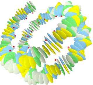
Let us first consider how these high affinity sequences are generated. In the model of Eslami-Mossalam et al., the DNA is constrained by binding 28 specific phosphates from the backbone of the DNA to the histone core. These binding sites force the DNA into a left-handed superhelical conformation, imitating the actual wrapping (see fig. 2.1). The base pairs are then assumed to be rigid bodies, as is common in modelling the mechan-ical properties of DNA ([16], [17]). Each combination of either AT or GC acts as a rigid plate as the hydrogen bonds connecting the two nucleotides are relatively strong. The freedom in this model lies in the orientation and positioning of these plates. Based on the wrapping and intrinsic twisting of the DNA it is assumed that the positioning and orientation have preferred or equilibrium values. Any change of conformation away from these equilibrium values will cost energy quadratic in the deformation. In rigid base pair models the exact parameters involved are then obtained either from experi-mental work or molecular dynamics (MD) simulations. In this model, the parameters used are from [18]. The authors of this paper combine existing parametrisations of elas-tic potentials for DNA to derive elaselas-tic free energies. The resulting hybrid parametri-sation combines elements derived from both MD simulations and structural data (e.g. crystal ensembles).
Since the base pairs are considered to be independent one might be worried as to how higher-order effects (di-/trinucleotide probabilities) can be extracted from these simulations. However, adjacent base pairs are in fact correlated through their equi-librium position, as these depend on the preceding part of the sequence. In biological terms, the base pairs are linked through the sugar-phosphate backbone of the DNA. The authors of [18] remark that including higher-order correlations has a relatively small ef-fect on the parametrisation.
Figure 2.1:Wrapped DNA modelled as rigid base pairs. Red dots indicate phosphates bound to the histone core.
What can be done however, is to generate an ensemble of high affinity sequences through an adapted Metropolis algorithm. The algorithm is a Markov chain Monte Carlo method that uses sampling from a probability distribution defined on the sample space. The algorithm attempts to move about this sample space accepting or rejecting the move based on the ratio of initial and final probabilities. As such it is a useful tool to approach the (local) minima of functions. In this case it is used to probe the sample space of conformations with the aim of finding an energetically favourable sequence. This is done by not only making changes to the configuration, but also allowing sponta-neous mutations of individual bases (base pairs). This mutation Monte Carlo algorithm (MMC) thus optimises both in configuration space and sequence space simultaneously. The MMC (and variations thereof as used in this paper) will be further elaborated upon in section 2.2. Using the MMC an ensemble of 107high affinity sequences was produced at 1/6 of room temperature. From these sequences the probabilities of occurrence of oligonucleotides can be calculated. These highlight the periodic preferences of nucleo-somal binding.
2.1.2
A probabilistic approximation
energies between the full model and the probabilistic model are calculated for chro-mosome I of S. cerevisiae. There is an excellent agreement with a root-mean-square deviation of only 0.85kBTR.
Let us now turn to how such a sequence probability is constructed. The total prob-ability of a given sequence is the probprob-ability of the combination of 147 base pairs that make up the sequence. By the chain rule of probability this becomes the product of conditional probabilities as given below.
P(S) = P( 147
\
i=1
Si) =
147
∏
n=1
P(Sn| n−1
\
i=1
Si) (2.1)
We can now make the assumption that the probability of each nucleotide depends only on the preceding nucleotide (instead of the entire preceding part of the sequence), as is also done by Segal et al. This gives:
P(S) = P(S1) 147
∏
n=2
P(Sn|Sn−1) (2.2)
Using that P(Sn|Sn−1) = P(Sn∩Sn−1)/P(Sn−1)we can rewrite the above equation
as:
P(S) = P(S1) 147
∏
n=2
P(Sn∩Sn−1)
P(Sn−1)
= ∏ 147
n=2P(Sn∩Sn−1)
∏146
n=2P(Sn)
(2.3)
We can also extend this and take the probability of each nucleotide to be dependent on the previous two nucleotides (see [15]). In this case the joint probabilities of three adjacent nucleotides need to be considered and eq 2.1 becomes:
P(S) = ∏ 147
n=3P(Sn∩Sn−1∩Sn−2)
∏146
n=3P(Sn∩Sn−1)
(2.4)
At this point the oligonucleotide probabilities can be calculated from the ensemble of high affinity sequences and used as input. In the case of the mononucleotide probability this is just the probability of having nucleotideSat positionn: P(Sn). The dinucleotide probabilities are the joint probabilities P(Sn∩Sn−1). Similarly the trinucleotide
prob-abilities are P(Sn ∩Sn−1∩Sn−2). This trinucleotide version of the probabilistic model
(equation 2.4) is used throughout this thesis unless explicitly stated.
2.2
Synonymous Mutation Monte Carlo
histone-DNA interaction energy, thus being able to theoretically position a nucleosome with bp precision? In order to do so we apply a variation of the MMC introduced by Eslami-Mossalam et al. namely the synonymous Mutation Monte Carlo algorithm (sMMC). Where the MMC changed individual bases, the sMMC exchanges synony-mous codons again according to a Metropolis algorithm. Since this is a probabilistic model the algorithm no longer explores configuration space (as for the full model), only sequence space. It is this novel approach of using a probabilistic model to explore se-quence space that will allow us to apply the algorithm on an almost genome-wide level.
In the first step a synonymous codon is selected for a random codon on the nu-cleosome. The move is accepted if the new codon increases the overall probability of the sequence for that specific nucleosome position (or keeps it constant). Alternatively, if the sequence probability is decreased by the new codon the move is accepted with probabilityPf/Pi or rejected with 1−Pf/Pi. Here Pi is the probability of the sequence with the initial codon and Pf is the probability of the sequence with the new codon. If the nucleosome starts at the 0 codon frame (the first bp on the nucleosome is the start of a codon) then there are a total of 49 codons on the nucleosome that can possibly be exchanged for a synonymous one. If the nucleosome starts at the 1 or 2 codon frame then the first and last codon are only partially on the nucleosome, but none the less con-tribute to the interaction energy. We then have 50 codons that can be changed.
To investigate to what degree DNA can be synonymously changed to affect nucle-osome affinity we will first apply the above algorithm to all possible nuclenucle-osome posi-tions on the YAL002W gene located on chromosome I of the S. cerevisiae genome and subsequently to all nucleosome positions of all S. cerevisiae coding sequences. All S. cerevisiae data was acquired from ensembl.org (genome version R64-1-1). YAL002W consists of 3825 base pairs which is about twice the average S. cerevisiae gene length [19] and should thus serve as a good representative. Furthermore the organism S. cere-visiae was also used in [12] and is therefore the obvious choice.
2.2.1
Parameter determination
Implicit in the model is the temperature at which the individual mono-, di- or trin-ucleotide probabilities are determined. This is not the actual temperature inside the nucleus but a simulation-technical parameter affecting how strongly certain states are preferred. Since all possible sequences are a canonical ensemble each state of the se-quence has a probability according to the Boltzmann distribution:
P = 1
Ze
−E/kBT and thus Pf Pi
P
f
Pi
TA/TB
=e−(Ef−Ei)/kBTB (2.6) While the model is formulated in terms of probabilities, it is more instructive to translate this into energies. For one, these can be compared to energetics models such as the model the input probabilities are derived from [15]. More importantly, sequence probabilities often differ by a couple of orders of magnitude making it hard to compare them as the highest probability will dominate any plot. Since the energy is given by the log of the probability (see eq. 2.7) comparing energies is much more informative as these can be readily plotted to visualise the mechanical properties of a sequence. From the above equation we get:
E =−kBT(log(P) +log(Z)) or forT = 1 6TR :
E kBTR
=−1
6log(P) +C (2.7)
HereTRthe room temperature andCis a constant depending on the normalisation. Since it is a constant shift and we are interested in relative affinities it will not be in-cluded in plots. To compare energies to different models one would have to make sure that the normalisation is the same for both models. Furthermore, all energies will be given in units ofkBTRso they are proportional to−log(P).
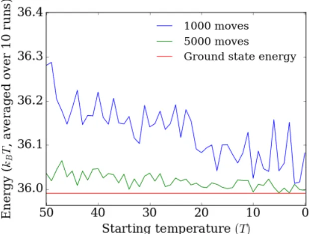
To test what temperature is best suited to quickly reach an acceptably low energy the sMMC was run for 1000 and 5000 moves at different temperatures (figure 2.2). Here the absolute lowest energy that a sequence can attain (given a free choice of all its synony-mous codons) is included. We call this the ground state energy of that sequence. It can be determined by way of a shortest path algorithm where the edges of the network are the different synonymous codons for each codon position. The weight of these edges is the energy attributed to each choice of codon and thus the algorithm will precisely pick out the path with the lowest possible energy.
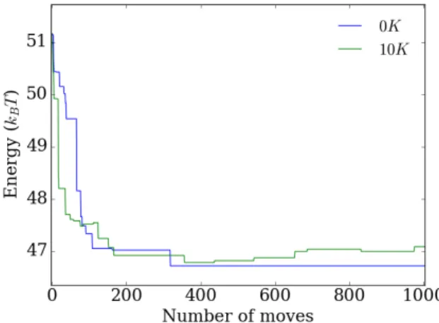
We see that the final interaction energy doesn’t change significantly from 1000 to 5000 moves, but that it does decrease as the temperature decreases. This suggests that there are very few local minima in the energy landscape, which means that a low temperature can be used to minimise fluctuations and effectively lower the energy as rapidly as possible. The sMMC was performed at position 56 of the YAL002W gene as it is a maximum of the nucleosome energy landscape. Throughout the following sections this position will often be chosen to consistently compare different methods.
Figure 2.2:DNA-histone interaction energy after 1000 (blue line) and 5000 (green line) sMMC moves for different temperatures at position 56 on the YAL002W gene. The red line is the
ground state energy. For each temperature the energy is averaged over 10 runs.
For the simulated annealing the final interaction energy is more or less independent of the starting temperature. This is likely due to the fact that as the temperature is low-ered the background fluctuations are less and less significant. This is especially clear for the 5000 moves simulation as the last 1000 moves are at a temperature of 10K or lower. From the previous figure we see that in this region the final energy starts to approach the ground state. We see that both after 1000 and 5000 moves the energy is close to the ground state energy with the longer simulation being the closest as is to be expected. For the longer simulation this final energy does not differ significantly from the simu-lation for constant low temperature (0K) in the previous figure. We therefore conclude that using simulated annealing doesn’t provide any advantages over choosing a suit-able low starting temperature.
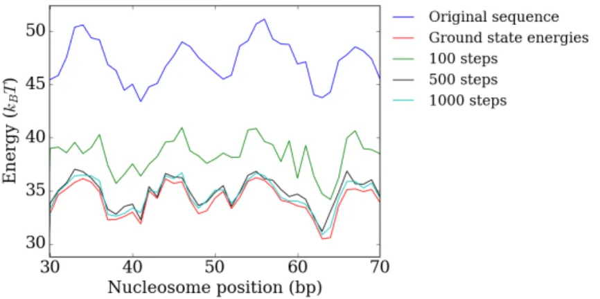
Next we examine the simulation run length. To get an indication of how the energy is lowered as the amount of moves is increased we plot the final energy of different po-sitions (figure 2.4). Here each point represents the final energy after running the sMMC for that nucleosome position andnotthe energy landscape after running the sMMC for one specific nucleosome position. Similarly for each position the ground state energy is separately calculated. We see that there is a significant difference in final energies be-tween 100 and 500 moves. However increasing the simulation length from 500 to 1000 moves hardly lowers the final energy.
Figure 2.3:Interaction energy after 1000 (blue line) and 5000 (green line) sMMC moves for different starting temperatures of the annealing schedule at position 56 on the YAL002W gene.
The red line is the ground state energy.
in a local minimum that is nevertheless very close to the global minimum. At 10K the energy fluctuates around a slightly higher equilibrium value but occasionally reaches the true global minimum. At 50K the energy fluctuates around an equilibrium value that is significantly higher than at a temperature of 10K and lower.
Figure 2.4:Interaction energy for different positions on the YAL002W gene after 100 (green line), 500 (black line) and 1000 (light blue line) sMMC moves at10K. The red line gives the
ground state energy for each position.
Figure 2.5:Change of the interaction energy during the simulation for different temperatures at position 56 on the YAL002W gene. The red line is ground state energy.
2.2.2
Results
With the above parameters we can now take a look at the energy landscape of a section of the YAL002W gene after running the sMMC simulation. Such an energy landscape is created by calculating the energy required to place a nucleosome (in this case the starting point of a nucleosome) at each base pair position along a sequence. The sMMC simulation changes a sequence of 147 base pairs (150 for overhanging codons on the nucleosome). The new energy landscape is then calculated for this new synonymous sequence. This new landscape will differ from the original one for all nucleosome po-sitions that encompass at least a part of the changed codons (i.e. nucleosome popo-sitions
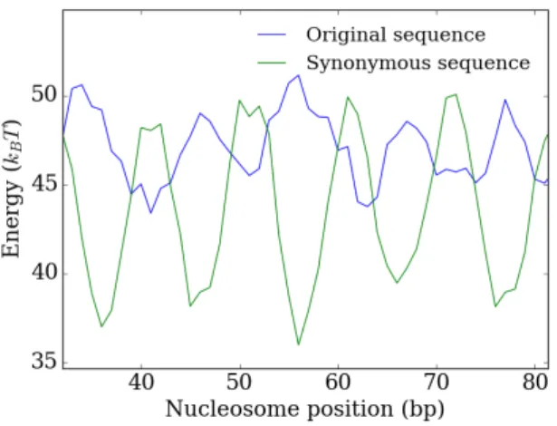
Figure 2.6:Original (blue) and synonymous (green, optimised at nucleosome starting position 56) DNA-histone interaction energy landscapes of a section of the YAL002W gene.
In figure 2.6 we see that at position 56, previously a maximum of the energy land-scape, the synonymous sequence now has a minimum. Again, although the interaction energy is only optimised for this position (the sequence of base pairs 56 through 202) we can see the characteristic 10 bp oscillations in the energy landscape for nucleosome positions where part of the aforementioned 147 base pairs is wrapped around the nu-cleosome.
Next we checked if a minimum could be reached for every nucleosome position on the YAL002W gene (save for the first and last 5 positions, the reason for this will become apparent shortly). As the nucleosome landscape naturally has an oscillation of about 10 to 11 bp we define a minimum to be a position such that the previous and next 5 nucleosome positions have higher energy. At each individual nucleosome position the sMMC simulation was run and for these synonymous sequences the interaction energy of nearby nucleosome positions was calculated to check if the optimised position is indeed a minimum. The results for different temperatures are listed in table 2.1 below.
Temp. (K) # of non-minimum positions % of correct minima
0 319 91.3
10 207 94.4
50 167 95.5
100 336 90.8
Table 2.1:Percentage of minima positions of the YAL002W gene after sMMC of 1000 moves at different temperatures.
to the optimised position. The figure on the right is a zoomed in version of the bottom part of the histogram. We can see that relatively few minima are at a distance of 1 bp from the optimised position and even fewer at a distance of 2 bp.
Figure 2.7:Left: Histogram of distance from local minima for each nucleosome position on the YAL002W gene. At each position the sMMC was run for a maximum of 1000 moves at a temperature of 50K (tot. number of positions is 3669). Right: Zoom in of the bottom part of the
histogram.
A possible explanation for the fact that the number of minima is highest at a temper-ature of 50K is that the goal is not only to have an energy that is as low as possible, but also one that is lower than that of the adjacent nucleosome positions. These adjacent nucleosome positions consist of almost the same sequence, only shifted by a few base pairs. Therefore the corresponding energy will conceivably also be lowered as the se-quences are so very similar. For some positions this actually turns out to be lower than the energy of the position that is being minimised. At a higher temperature there may be a little more leeway. That is the energy of positionxis not lowered as effectively, but as a result the adjacent positions don’t surpass it.
Figure 2.8:Left: Histogram of distance from local minima for each nucleosome position of all S. cerevisiae genes. At each position the sMMC was run for a maximum of 1000 moves at a
temperature of 50K. Right: Zoom in of the bottom part of the histogram.
2.3
Frequency dependent sMMC (fsMMC)
2.3.1
The codon bias phenomenon
It has been shown for various organisms that different synonymous codons occur with different frequencies [20]. This disparity is known as codon bias [21]. Even though syn-onymous codons encode for the same amino acid, apparently there is some discriminat-ing force resultdiscriminat-ing in certain codons occurrdiscriminat-ing more often than others. In fast-growdiscriminat-ing microorganisms like E. coli or our S. cerevisiae this disparity in the codon frequencies is mirrored in the composition of the tRNA pool ([22], [23]). The two most widely ac-cepted explanations for this difference in frequencies are mutational bias and natural selection. In the selectionist view the choice in codon affects the gene expression and is therefore subject to natural selection. This is supported, among other reasons, by the fact that more frequent codons are recognized by more abundant tRNAs [24]. The mu-tational explanation on the other hand states that the codon bias is simply a result of an underlying mutational bias. Since certain mutations occur more frequently than oth-ers, some codons are more apt to change into others resulting in a shift in equilibrium frequencies. Neither can fully explain all the features of codon bias and it is therefore thought that the bias arises from a combination of both natural selection and mutational bias [25] [26].
will take different approaches to incorporating a constraint aimed at keeping codon fre-quencies similar.
Apart from the biological reasons to take this codon bias into account it can serve as an interesting constraint on the synonymous codon exchange to investigate how flexible this process is and if similar results can be achieved even under stricter constraints. For the cutoff fsMMC the table of codon frequencies was acquired fromhttp://downloads. yeastgenome.org/unpublished_data/codon/ysc.gene.cod. This table was produced using only open reading frames (ORFs) that have been assigned a gene name. This in-cluded 3,222 ORFs out of the total of 6,219 that are contained within the Saccharomyces Genome Database (SGD) as of January 1999.
In the above considerations we have not taken into account the wobble hypothesis. This states that some of the third nucleotides of the mRNA not only conform to the original Watson-Crick pairing but can also be recognised by some other anti-codon base pairs of the tRNA 5’ site. The reason why we have not taken this into account is that the wobble position only affect the size of the tRNA pool that can recognise a certain mRNA codon and is not directly linked to the codon frequencies.
2.3.2
Cutoff fsMMC
The first and easiest approach is to limit the frequency difference that any two synony-mous codons can have to be eligible for exchange. This imposed cutoff of the frequency difference ensures that a frequent codon won’t be replaced by a rare one. This is espe-cially important should this indeed have an effect on the translation elongation speed and consequently possibly also on cotranslational folding.
As an example, the table below lists the fractions of occurrence for the different codons encoding for proline.
Codon Fraction
CCG 0.12
CCA 0.42
CCT 0.31
CCC 0.15
Table 2.2:Fractions for the different codons encoding for proline.
moves but might not practically differ a lot from the regular sMMC.
Figure 2.9:Energy change at position 56 of the YAL002W gene during fsMMC with a cutoff frequency difference of 0.05 at a temperature of 0K (blue line) and 10K (green line).
Let us first consider a strict cutoff of 0.05 and see if the change in energy can compare to the unconstrained sMMC. The results are plotted in figure 2.9 for both 0 and 10K. It is clear that there are a lot less moves allowed than in the unconstrained case as the energy only reaches a value of around 47kBTRwhereas this was 36kBTRfor the sMMC.
Next, in figure 2.10 the histone-DNA interaction energy landscapes are plotted after running the fsMMC for different cutoff values of the frequency difference (optimised at position 56). We see that for a very strict cutoff value of 0.05 (left subfigure) the sequence is unable to change enough for a minimum to appear in the landscape. For a value of 0.1 (middle subfigure) there is a minimum at position 56 although it is not as deep as the 0.2 or sMMC one. For the cutoff value of 0.2 we can see that the nucleosome landscape is very similar to that of the regular sMMC. This can be explained by again using the table (2.2) of proline codons as an example: for a cutoff of 0.05 only two codons can be exchanged, for 0.1 two pairs of codons can be exchanged and for 0.2 almost all codons can be freely exchanged. The latter will therefore be very similar to the regular sMMC.
Figure 2.10:Nucleosome landscapes for fsMMC with a cutoff frequency difference of 0.05 (left), 0.1 (middle) and 0.2 (right) at position 56 of the YAL002W gene for 1000 moves at a
temperature of 0K.
Figure 2.11:Histograms of distance from local minima for each nucleosome position on the YAL002W gene. At each position the fsMMC was run for a maximum of 10.000 moves at a
temperature of 10K. Left: Cutoff frequency of 0.05. Middle: Cutoff frequency of 0.1. Right: Cutoff frequency of 0.2.
2.3.3
Codon swapping fsMMC
testing the applicability of this method with an imposed constraint. In particular it pro-vides us with a method that allows us to investigate how the sMMC performs while keeping the codon frequencies constant (at least on a∼150 bp scale).
To implement this, the sMMC can simply be changed so that for some codon on the nucleosome a synonymous codon elsewhere on the nucleosome is now selected (instead of selecting an arbitrary synonymous codon). The move is then accepted or rejected again according to the probability of the entire sequence. Note that the new sequence is now changed in two locations simultaneously.
Figure 2.12:Original (blue) and synonymous (green) DNA-histone interaction energy landscapes of a section of the YAL002W gene. The synonymous sequence is the result of the
codon swapping sMMC at position 56 for 1000 moves at 10K.
Figure 2.13:Interaction energy for different positions on the YAL002W gene after codon swapping sMMC for 1000 moves at10K. The red line gives the ground state energy for each
position.
Figure 2.14:Histogram of distance from local minimum for each nucleosome position on the YAL002W gene. At each position the codon swapping sMMC was run for a maximum of 5000
moves at a temperature of 10K.
2.4
Deterministic codon changes
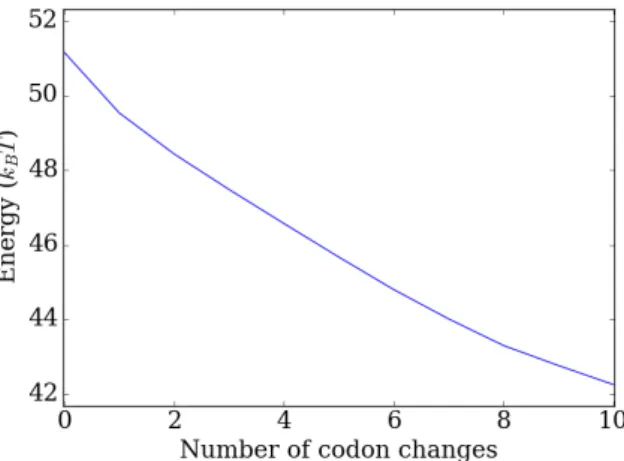
the first place as opposed to, say, looking at the ground state energies. In this section however, we will investigate how rapidly a minimum can be reached when determin-istically changing codons. While evolution is stochastic in nature, this deterministic approach will serve to explore how much the energy landscape can be altered with just a few changes to the sequence. Furthermore, should the selective pressure be high enough a small change in the sequence might be highly favoured if it has a large impact on nucleosome positioning.
In order to lower the nucleosome energy as swiftly as possible the codon exchange that was the most energetically favourable (out of all the codons on the nucleosome and all their synonymous codons) was made. This step was then repeated up to 50 times. The selected codons were exchanged for any synonymous one without any constraints on the frequencies.
Figure 2.15:Energy change at position 56 of the YAL002W gene for 10 consecutive determinstic codon changes.
Figure 2.16: Original (blue) and synonymous (green) energy landscapes of a section of the YAL002W gene. The synonymous sequence was changed through 10 deterministic codon
exchanges.
Figure 2.17:Left: Histogram of distance from local minima for each nucleosome position on the YAL002W gene for up to 50 codon changes. Right: histogram of the number of changes needed
Chapter
3
Codon usage in high nucleosome
occupancy regions
In section 2.3.1 the codon usage bias phenomenon was addressed, which states that synonymous codons encoding for the same amino acid occur with different frequen-cies. These frequencies are usually calculated genome wide or among genes to compare them. However, it is not often investigated if they diverge locally from this ‘equilib-rium’ frequency. While in the previous chapter we sought to change a sequence syn-onymously to increase nucleosome affinity, we will now investigate if certain codons are indeed more prevalent in high nucleosome occupancy regions. It has been shown both in vivo and in vitro for many different organisms that there is a distinct dip in nucleosome occupancy (averaged over all genes) just before the transcription start site (TSS) and a peak just after the TSS [14]. In this chapter we therefore investigate the frequency of occurrence of all codons from the transcription start site onwards. This is done per base pair position and averaged over all genes for different organisms. Apart from S. cerevisiae we also look at the nematode Caenorhabditis elegans, as it has a more pronounced occupancy peak close to the TSS, and the ciliate Tetrahymena thermophila, as it was recently used in a study of nucleosome patterns within coding regions [29].
3.1
Data acquisition
3.2
Method
To calculate the codon usage on these genes we only look at the coding sequences (CDS) that ultimately get translated into protein. That is, the introns and 5’/3’ untranslated regions (UTR) were ignored since they do not get translated and thus do not contain codons. However, only the original location of each codon relative to the TSS on the transcribed sequence, and not its relative position within the CDS, can be compared to other quantities such as the nucleosome occupancy per position (see figure 3.1). So it is this relative position that was used when aggregating all codon counts. In keeping with previous conventions we take the position of a codon to be the position of its first base pair.
Figure 3.1:Schematic representation of an unspliced gene transcript. Untranslated base pairs are denoted by lower case letters in either the UTR (green) or introns (gray), while translated base pairs in coding regions (orange) are upper case. Base pairs highlighted in red indicate the
start of a codon with a well-defined position.
One minor problem with this indexing is that it is not uncommon for codons to span two exons. For example, a codon could have its first base pair at the end of one exon and its second and third base pairs at the start of the following exon (e.g. the CTA codon in fig. 3.1). Since all exons are ligated before translation this does not matter for the codon-tRNA pairing step in the translation. For our purposes however, these codons have to be discarded as their position is not well-defined. All of the remaining codons were counted per position relative to the TSS and normalised according to the total number of counts among the synonymous codons to get their codon frequency. In the case of T. thermophila, a lot of the genes are positioned very close to the start or end of a scaffold (since these are relatively short, as explained in 3.3.3). This means that the occupancy signal cannot be calculated for some base pair positions of these genes. To rectify this disparity the average was simply calculated at each individual position according to the number of occupancy values for that specific position.
can only really be determined for these positions. The few codons that do start in the 1 or 2 reading frame don’t provide enough data to give an accurate average and have to be discarded. In all plots of S. cerevisiae codon usage the frequency is therefore only plotted at positions that are in the 0 reading frame (multiples of 3). In C. elegans and T. thermophila, on the other hand, almost every gene has multiple introns. This means that there are consistently enough codons in all reading frames to calculate meaningful averages for all positions.
The codon frequencies are then compared to nucleosome occupancy and, as a proxy, GC content. The nucleosome occupancy can be determined in a number of ways. For C. elegans we compare with experimental in vivo (from [30]) and in vitro data (from [31]) and predicted nucleosome occupancy as is done by Tompitak et al. [14]. This predicted nucleosome occupancy is calculated using the trinucleotide model from chapter 1. The input probabilities used were changed from those acquired from the hybrid parametri-sation to a parametriparametri-sation informed solely by crystallography data [32]. Tompitak et al. note that Becker et al. [18], in testing the different parametrisations, only use short sequences. The stiffness parameters in the hybrid model are based on MD simulations, which seem to perform best for modelling local nucleosome affinity. However, deriving them from crystallography data has improved applicability to long-range effects and is therefore more suited for this type of research. The sequences used start 146 bp up-stream from the TSS and continue to bp 646. For each of these sequences the probability landscape is calculated. The occupancy for any base pair is then taken to be the sum of the log of the probabilities of all possible 147 nucleosomes that base pair is a part of. This results in an occupancy signal for the first 500 bp downstream of the TSS. These oc-cupancy signals are then averaged over all genes and subsequently normalised so that the signal sums to 0.
It has been shown that GC content correlates with nucleosome affinity and occu-pancy ([33], [34]) so it stands to reason that, in regions with varying occuoccu-pancy, the balance in codon frequencies might shift to reflect any change in GC content [35]. This should hold true especially for GC3, which is the GC content in the third codon reading
3.3
Results
3.3.1
S. cerevisiae
Let us first take a look at the results for S. cerevisiae. Figure 3.2 shows the GC content 1000 bp upstream and downstream from the transcription start site averaged over all genes. We can clearly see the previously mentioned drop in GC content just before the TSS. Unfortunately this region doesn’t have any codons, as it isn’t part of the subsequent gene and so what is really the more interesting part of the GC profile is useless for our purposes. The sharp spikes at position 0, 1 and 2 correspond with the frequency of A, T and G respectively (the start codon) which are present at these positions for almost all genes of S. cerevisiae. The GC content from the TSS onward fluctuates tremendously and has only a very minor overall decline. This becomes more apparent in the right-hand figure of 3.2 which is the GC content for 500 bp positions downstream of the TSS. Apart from a very minor dip the first 40 base pairs the GC content is almost constant save for local fluctuations.
Figure 3.2:Left: GC content per bp for 1000 bp upstream and downstream from the TSS, averaged over all S. cerevisiae genes. Right: Zoom of the left plot for the first 500 bp
downstream of the TSS.
Figure 3.3:Relative frequency of the synonymous codons encoding for Phenylalanine for the first 500 bp downstream of the TSS, averaged over all S. cerevisiae genes.
3.3.2
C. elegans
For this reason C. elegans is an organism that is more suited for our purposes. In a plot of the GC content (left of fig. 3.4) we see that C. elegans has both a drop before the TSS and a peak after the TSS. The same is true for the in vivo, in vitro and predicted nucleosome occupancy (this is the same as figure 1D in [14]). The right-hand figure shows that this peak is a very distinct feature of about 100 bp after the TSS. Similarly the nucleosome occupancies have a slightly shifted peak due to the averaging over all nucleosomes per base pair position (which is why GC content gives a more accurate representation of local nucleosome affinity). Also the GC content of C. elegans has con-siderably fewer fluctuations than that of S. cerevisiae, which might result in smoother codon frequencies.
Figure 3.4:Top left: GC content averaged over all C. elegans genes, 1000 bp upstream and downstream from the TSS. Top right: Zoom of the left plot for the first 500 bp downstream of the TSS. Bottom left: Predicted (blue), in vitro (red, [31]) and in vivo (green, [30]) nucleosome
occupancy. Bottom right: Zoom of the left plot for the first 500 bp.
bp and conversely an increase in AAT. The frequencies fluctuate a lot however, which is most likely due to the limited amount of data combined with the fact that not all codons will occur as often at every position. Another reason could be that if there are sufficient specifically bound nucleosomes in this region that the codon frequencies might mirror the 10 bp periodic binding preference [39]. From the occupancy plots it is of course clear that there are on average more nucleosomes just after the TSS than in adjacent regions. However, by specifically bound it is meant that nucleosome positioning (relative to the TSS) differs by only a few bp (or any multiple of 10) for a significant amount of nucle-osomes so that the periodic preferences are reflected even when averaging. In order to straighten out these fluctuations we average over the preceding and following 5 codon positions. This results in a much smoother plot that makes it easier to distinguish be-tween local fluctuations and meaningful trends (right of fig. 3.5). This smoothing will be done for all of the following codon plots.
Figure 3.5:Left: Relative frequency of the synonymous codons encoding for Asparagine for the first 500 bp downstream of the TSS, averaged over all C. elegans genes. Right: Smoothed version of the plot on the left by averaging over the previous and following 5 codon positions.
For most of the amino acids encoded by more than two codons there are so many variables in play that is it hard to discern any underlying patterns (see appendix A). However, even for some of the amino acids encoded by four codons the same patterns can be observed. Figure 3.6 shows the relative frequency of the codons encoding for Threonine for the first 500 bp downstream of the TSS. Again we can see a decrease in the frequency of codons with higher GC content (ACC and ACG) and an increase in codons with lower GC content (ACT and ACA) over the first 100 bp.
Figure 3.6:Smoothed plot (by averaging over the surrounding 10 codon positions) of the synonymous codons encoding for Threonine for the first 500 bp downstream of the TSS,
averaged over all C. elegans genes.
Figure 3.7:Left: Relative frequency of the synonymous codons encoding for Glutamine for the first 500 bp downstream of the TSS, averaged over all C. elegans genes. Right: Smoothed version of the plot on the left by averaging over the previous and following 5 codon positions.
Note that the codon with lower GC count is more frequent for the first 100 bp.
3.3.3
T. thermophila
Lastly, the ciliate Tetrahymena thermophila was examined. T. thermophila exhibits a few peculiarities not found in other eukaryotes. Firstly, like al protozoan ciliates it has two types of nuclei, a phenomenon which is called nuclear dimorphism. These nu-clei perform different tasks: the micronucleus is germline-like and is solely used for reproduction purposes and the macronucleus is soma-like and controls metabolism. Furthermore, this polyploid macronucleus is derived from the diploid micronucleus. When forming the macronucleus the five chromosomes of the micronucleus are copied numerous times and subsequently develop into micro-chromosomes by deletion of in-ternally eliminated sequences (among other processes). The possible overlap of these micro-chromosomes makes shotgun sequencing a strenuous process. Instead contigs (that represent a consensus region of DNA readings) are pieces together to form larger scaffolds. These scaffolds are likely to represent (part) of a macronucleus chromosome [40]. In the data set used 1158 of such scaffolds have been identified. A second pecu-liarity of the T. thermophila genome is that the stop codon is only encoded by TGA. The two codons TAA and TAG used as stop codons in most other eukaryotes have been reassigned to Glutamine.
Figure 3.8:GC content for the first 500 bp downstream of the TSS, averaged over all T. thermophila genes.
Beh et al. [29] constructed a genome wide nucleosome map of all in vitro and in vivo nucleosomes of T. thermophila in order to investigate the difference between DNA-guided nucleosomes and trans factor-guided nucleosomes. They find that T. ther-mophila exhibits a stereotypical nucleosome array downstream of the TSS, both in vitro and in vivo. Such a pattern is found in most unicellular eukaryotes, where regular spaced nucleosomes follow a nucleosome depleted region (located just before the TSS, [14]). Averaging over genes with different nucleosome arrays then results in an occu-pancy plot such as figure 3.8. S. cerevisiae differs from T. thermophila in the sense that such an array is only present in vivo and not in vitro. As it is generally agreed upon that in vitro nucleosome patters stem from DNA-guided nucleosomes and in vivo patterns from a combination of both DNA-guided and trans factor-guided nucleosomes, taking a closer look at genes with these specific nucleosome patters might prove insightful. Beh et al. note that aggregate analysis of genomic data can be misleading as indiscriminate averaging can smooth out features of importance. To this end they look at individual genes and determine whether it has a nucleosome at so called ‘standard’ positions, see figure 3.9. These standard positions are the most common nucleosome positions down-stream of the TSS and are denoted as either +1, +2 or +3 (located within a±35 window of bp +122, +310 and +505 resp. for in vitro positioned nucleosomes). Of all possible combinations of standard nucleosomes found on individual genes a +1, +1 and +2 or +1, +2 and +3 are most prevalent. To that end they compiled a list of genes with either one, two, three or lacking a standard nucleosome. These were comprised of 995, 716, 664 and 1695 genes respectively. Figure 3.10 shows the GC content of these four classifications of genes (in [29] this is figure 4, comparing this to the in vitro and in vivo nucleosome positioning). It is clear that at the sites of these standard nucleosomes the GC content is higher on average.
Figure 3.9:Schematic representation of standard +1, +2 and +3 nucleosome positions vs. non-standard nucleosome positions (figure 3 in [29]).
Figure 3.10:GC content for the first 600 bp downstream of the TSS, averaged over T. thermophila genes with either no nucleosome (top left), a +1 nucleosome (top right), a +1 and
+2 nucleosome (bottom left) or a +1, +2 and +3 nucleosome (bottom right) as called by Beh et al. [29]
patterns of figure 3.10, albeit distorted with a lot of fluctuations. Keep in mind that each of these plots are generated from considerably fewer genes than those of C. elegans and consequently there will be even fewer reads of each codon per position. As such it is not surprising that there are more local fluctuations. The codon with the highest GC content (AAC) seems to occur more frequently at standard nucleosome positions, as is to be expected. Conversely AAT is less prevalent at these positions.
Figure 3.11:Relative frequency of the synonymous codons encoding for Asparagine for the first 600 bp downstream of the TSS, averaged over all T. thermophila genes with either no (top
left), one (top right), two (bottom left) or three (bottom right) standard nucleosomes. (Smoothed by averaging over the previous and following 5 codon positions)
taken into account.
For T. thermophila (and to a lesser extent C. elegans), one would ideally like some statistical method to compare the (approximate) shape of the GC content curve and that of the codon frequencies. There are a few problems with this however. Firstly, these are not well defined curves. The ample fluctuations, even when averaged, would throw off any kind of point by point comparison such as a measure of distance (e.g. Hausdorff dis-tance). Secondly, and most importantly, such an absolute comparison would not even make sense as the curves are not part of the same metric space. Any codon frequency is dependent on the frequencies of its synonymous codons. Only the relative increase of a codon can be compared to the increase relative increase of GC content. Therefore the best that can be done is comparing the codon frequency within and outside of nucleo-some domains. As stated earlier Beh et al. already did this. So unfortunately a visual comparison of the curves seems to be the only possibility.
3.3.4
Conclusion
Chapter
4
Discussion
In the first chapter it was shown that it is indeed theoretically possible to significantly change the nucleosome affinity of a sequence by only changing synonymous codons. From this it is tempting to draw the conclusion that something similar can be seen in C. elegans. The genetic sequence just downstream of the TSS seems to differ from other re-gions to accommodate (DNA-guided) nucleosomes. By accumulation of specific codons the nucleosome affinity (and also the GC content) of the sequence is increased.
There are some caveats that bear mentioning, however. The first chapter explores the possibility of synonymously altering a sequence to place nucleosomes with bp pre-cision. This is done by lowering the histone-DNA interaction energy for a specific nu-cleosome position through sMMC, but without any regard for adjacent positions. As mentioned previously the reason a Metroplis algorithm is used as opposed to consid-ering the ground state energies for each position is that it somewhat resembles evolu-tionary change. An obvious improvement to this would be to alter the algorithm so moves that lower the energy of adjacent positions have a higher penalty and are thus less likely to occur. On its own this feat functions more as an assessment of the possibil-ities offered by the inherent degeneracy of the genetic code for changing the mechanical properties of DNA. In C. elegans (and other multicellular organisms [14]) we see larger regions of nucleosome attraction. Even nucleosomes classified as having a standard po-sition are located somewhere within a 70 bp window. Thus, if such nucleosomes are DNA-guided it must be the result of these larger regions of gene sequences having an inherently favourable nucleosome affinity. Trying to recreate this and see if the posi-tioning rules are affected would be an interesting follow-up topic.
nu-cleosome this average increase is inconsequential however. Based on the affinity of an individual gene sequence the DNA will be wrapped around the histone complex thus forming a nucleosome. In other words, if this discriminating force is to be of any signif-icance it should be apparent from the individual gene. Classifying genes is one way of approaching this while still retaining the ability to compare and average, but also has its drawbacks due to the decreased sample size. It would be interesting to investigate this further in a future study.
Acknowledgements
I would like to express my gratitude to my supervisor Prof. dr. Helmut Schiessel for his guidance, our valuable discussions and for providing me with the opportunity of building on past research within his group of Theoretical Physics of Life Processes. I would also like to thank two group members in particular, Marco Tompitak for helping me get started with the computational work and our fruitful conversations and Martijn Zuiddam for providing me with his algorithm to calculate the ground state energy of a sequence.
Appendix
A
Additional figures
A.1
Caenorhabditis elegans
Figure A.1:Relative frequency of the synonymous codons encoding for different amino acids for the first 500 bp downstream of the TSS for both the original (left) and by averaging over the
Figure A.2:Relative frequency of the synonymous codons encoding for different amino acids for the first 500 bp downstream of the TSS for both the original (left) and by averaging over the
Figure A.3:Relative frequency of the synonymous codons encoding for different amino acids for the first 500 bp downstream of the TSS for both the original (left) and by averaging over the
Figure A.4:Relative frequency of the synonymous codons encoding for different amino acids for the first 500 bp downstream of the TSS for both the original (left) and by averaging over the
Figure A.5:Relative frequency of the synonymous codons encoding for different amino acids for the first 500 bp downstream of the TSS for both the original (left) and by averaging over the
Figure A.6:Relative frequency of the synonymous codons encoding for Valine for the first 500 bp downstream of the TSS for both the original (left) and by averaging over the closest 10
A.2
Sacheromices cerevisiae
A.3
Tetrahymena thermophila
Figure A.10:Relative frequency of the synonymous codons encoding for Aspartic acid for the first 600 bp downstream of the TSS, averaged over all T. thermophila genes with either no (top
Figure A.11:Relative frequency of the synonymous codons encoding for Tyrosine for the first 600 bp downstream of the TSS, averaged over all T. thermophila genes with either no (top left),
[1] K. Luger, A. W. M¨ader, R. K. Richmond, D. F. Sargent, and T. J. Richmond,Crystal structure of the nucleosome core particle at 2.8 ˚A resolution, Nature389, 251 (1997).
[2] T. J. Richmond and C. A. Davey,The structure of DNA in the nucleosome core, Nature
423, 145 (2003).
[3] K. E. Van Holde, Chromatin, Springer Science & Business Media, 2012.
[4] MBInfo contributors, Nucleosome is the first level of DNA packaging, https://www. mechanobio.info/figure/1389942837319/, Mechanobiology Institute, National University of Singapore.
[5] V. M. Studitsky, D. J. Clark, and G. Felsenfeld, Overcoming a nucleosomal barrier to transcription, Cell83, 19 (1995).
[6] K. Struhl and E. Segal, Determinants of nucleosome positioning, Nature structural & molecular biology20, 267 (2013).
[7] H. R. Drew and A. A. Travers,DNA bending and its relation to nucleosome positioning, Journal of molecular biology186, 773 (1985).
[8] P. Lowary and J. Widom,New DNA sequence rules for high affinity binding to histone octamer and sequence-directed nucleosome positioning, Journal of molecular biology
276, 19 (1998).
[9] J. C. Wang,Helical repeat of DNA in solution, Proceedings of the National Academy of Sciences76, 200 (1979).
[10] R. Wheeler, http://www.richardwheeler.net/contentpages/index.php.
[12] B. Eslami-Mossallam, R. D. Schram, M. Tompitak, J. van Noort, and H. Schiessel,
Multiplexing Genetic and Nucleosome Positioning Codes: A Computational Approach, PLOS ONE11, 1 (2016).
[13] E. Segal, Y. Fondufe-Mittendorf, L. Chen, A. Th˚astr ¨om, Y. Field, I. K. Moore, J.-P. Z. Wang, and J. Widom, A genomic code for nucleosome positioning, Nature 442, 772 (2006).
[14] M. Tompitak, C. Vaillant, and H. Schiessel,Genomes of Multicellular Organisms Have Evolved to Attract Nucleosomes to Promoter Regions, Biophysical Journal (2017).
[15] M. Tompitak, G. T. Barkema, and H. Schiessel,Benchmarking and refining probability-based models for nucleosome-DNA interaction, BMC bioinformatics18, 157 (2017).
[16] C. Calladine and H. Drew,A base-centred explanation of the B-to-A transition in DNA, Journal of molecular biology178, 773 (1984).
[17] B. D. Coleman, W. K. Olson, and D. Swigon,Theory of sequence-dependent DNA elas-ticity, The Journal of chemical physics118, 7127 (2003).
[18] N. B. Becker, L. Wolff, and R. Everaers,Indirect readout: detection of optimized subse-quences and calculation of relative binding affinities using different DNA elastic potentials, Nucleic acids research34, 5638 (2006).
[19] J. Zhang, Protein-length distributions for the three domains of life, Trends in Genetics
16, 107 (2000).
[20] R. Grantham, C. Gautier, M. Gouy, R. Mercier, and A. Pave,Codon catalog usage and the genome hypothesis, Nucleic acids research8, 197 (1980).
[21] R. Hershberg and D. A. Petrov, Selection on codon bias, Annual review of genetics
42, 287 (2008).
[22] T. Ikemura,Codon usage and tRNA content in unicellular and multicellular organisms., Molecular biology and evolution2, 13 (1985).
[23] S. Kanaya, Y. Yamada, M. Kinouchi, Y. Kudo, and T. Ikemura,Codon usage and tRNA genes in eukaryotes: correlation of codon usage diversity with translation efficiency and with CG-dinucleotide usage as assessed by multivariate analysis, Journal of molecular evolution53, 290 (2001).
[24] J. F. Curran and M. Yarus,Rates of aminoacyl-tRNA selection at 29 sense codons in vivo, Journal of molecular biology209, 65 (1989).
[25] M. Bulmer, The selection-mutation-drift theory of synonymous codon usage., Genetics
[26] D. C. Shields and P. M. Sharp,Synonymous codon usage in Bacillus subtilis reflects both translational selection and mutational biases, Nucleic Acids Research15, 8023 (1987).
[27] H. Akashi,Synonymous codon usage in Drosophila melanogaster: natural selection and translational accuracy., Genetics136, 927 (1994).
[28] M. A. Sørensen, C. Kurland, and S. Pedersen,Codon usage determines translation rate in Escherichia coli, Journal of molecular biology207, 365 (1989).
[29] L. Y. Beh, M. M. M ¨uller, T. W. Muir, N. Kaplan, and L. F. Landweber,DNA-guided es-tablishment of nucleosome patterns within coding regions of a eukaryotic genome, Genome research25, 1727 (2015).
[30] S. Ercan, Y. Lubling, E. Segal, and J. D. Lieb,High nucleosome occupancy is encoded at X-linked gene promoters in C. elegans, Genome research21, 237 (2011).
[31] G. Locke, D. Haberman, S. M. Johnson, and A. V. Morozov, Global remodeling of nucleosome positions in C. elegans, BMC genomics14, 284 (2013).
[32] W. K. Olson, A. A. Gorin, X.-J. Lu, L. M. Hock, and V. B. Zhurkin, DNA sequence-dependent deformability deduced from protein–DNA crystal complexes, Proceedings of the National Academy of Sciences95, 11163 (1998).
[33] N. Kaplan, T. R. Hughes, J. D. Lieb, J. Widom, and E. Segal, Contribution of histone sequence preferences to nucleosome organization: proposed definitions and methodology, Genome biology11, 140 (2010).
[34] D. Tillo and T. R. Hughes, G + C content dominates intrinsic nucleosome occupancy, BMC bioinformatics10, 442 (2009).
[35] M. D. Ermolaeva et al.,Synonymous codon usage in bacteria, Current issues in molec-ular biology3, 91 (2001).
[36] E. Elhaik and T. Tatarinova,GC3Biology in Eukaryotes and Prokaryotes, (2012).
[37] X.-F. Wan, D. Xu, A. Kleinhofs, and J. Zhou, Quantitative relationship between syn-onymous codon usage bias and GC composition across unicellular genomes, BMC Evolu-tionary Biology4, 19 (2004).
[38] Y. Zhang, Z. Moqtaderi, B. P. Rattner, G. Euskirchen, M. Snyder, J. T. Kadonaga, X. S. Liu, and K. Struhl,Intrinsic histone-DNA interactions are not the major determi-nant of nucleosome positions in vivo, Nature structural & molecular biology 16, 847 (2009).
[39] A. Klug and L. Lutter,The helical periodicity of DNA on the nucleosome, Nucleic acids research9, 4267 (1981).