DATA SCIENCE METHODS WITH APPLICATIONS TO GENETIC SEQUENCING
Weiwei Li
A dissertation submitted to the faculty at the University of North Carolina at Chapel Hill in partial fulfillment of the requirements for the degree of Doctor of Philosophy in the Department of
Statistics and Operations Research.
Chapel Hill 2020
c 2020 Weiwei Li
ABSTRACT
WEIWEI LI: Data Science Methods with Applications to Genetic Sequencing
(Under the direction of Jan Hannig, Corbin D. Jones, and Sayan Mukherjee)
Data science methods are of increasing importance in modern genetic sequencing analysis. In this dissertation, we focus on applying statistical modeling to structural variant detection problems and a new framework for scalable and provable subspace clustering.
We first discuss the optimal sampling strategy for structural variant detection using optical mapping. Here we develop an optimization approach using a simple, yet a realistic, model of the genomic mapping process using a Hypergeometric distribution and probabilistic concentration inequalities. Surprisingly we show that if a genomic mapping technology can sample most of the chromosomal fragments within a sample, comparatively little biological material is needed to detect a variant at high confidence.
In the second part, we introduce a formal probabilistic model to assessing how well an optical maps to a reference genome. We use this approach to infer the most likely location within that reference for any given read, as well as the likelihood of mapping to all other possible locations. Using data produced by BioNano Saphyr to parameterize a simulation, we show that our approach accurately identifies the likeliest locations of the observed optical read data. While considerably faster than a canonical MCMC approach, our approach is still computationally intensive. We provide several algorithmic improvements that increase the speed with no apparent impact on accuracy. Our approach provides a rigorous, open-source framework for analyzing optical read data.
ACKNOWLEDGEMENTS
It is a truth universally acknowledged, that a Ph.D. student in possession of a great graduate study, must be surrounded by many great people. Now my school life is coming to an end, and I would like to express my sincere gratitude to all the people who have contributed a lot to my awesome five years at Chapel Hill.
First and foremost, I am indebted to my advisors, Prof. Jan Hannig, Prof. Corbin D. Jones and Prof. Sayan Mukherjee. Thank you so much for your guidance and supports during my graduate study. Jan, I truly appreciate that you granted me the flexibility to expand my research interests and do internships in industry. I have learned a lot from our technical discussions and am constantly amazed by your innovative ideas. Corbin, your optimism personality makes my whole research experience enjoyable. It is inspiring to see an established professor like you still so humble and eager to learn new things. Sayan, thank you so much for accepting me as your student, I know it is very rare in Duke. I also feel grateful that you have broadened my vision in research and motivated me to explore more in the intersection of traditional statistics and computer science. In retrospect, I am so lucky to have you three as my advisors. Finishing graduate study is just another starting point of my new journey, and I believe one day, you will be very proud of me.
Besides my advisors, I would like to thank the rest of my dissertation committee members Professor Kai Zhang and Professor Nicolas Fraiman. Kai, I really enjoyed your course in generalized linear models, that course motivated me to think about linear models more from a plane perspective. Nicolas, I know that you have a very busy schedule this semester and thank you so much for taking the time to be my committee member.
TABLE OF CONTENTS
LIST OF TABLES . . . xi
LIST OF FIGURES . . . xii
CHAPTER 1: INTRODUCTION . . . 1
1.1 Optimal Sampling for Variant Detection . . . 1
1.2 Semi-Parametric Model for Optical Mapping . . . 2
1.3 Subspace Clustering through Sub-Clusters . . . 3
CHAPTER 2: OPTIMAL SAMPLING FOR VARIANT DETECTION . . . 4
2.1 Introduction . . . 4
2.2 Approach . . . 5
2.3 Statistical Model . . . 6
2.3.1 Analytical calculations . . . 8
2.3.2 Optimal sampling strategy . . . 10
2.4 Sampling algorithm . . . 11
2.4.1 Lower bound on K . . . 11
2.4.2 Lower bound on R . . . 12
2.5 Numerical results . . . 12
2.6 Conclusion . . . 15
CHAPTER 3: SEMI-PARAMETRIC MODEL FOR OPTICAL MAPPING . . . 16
3.1 Introduction . . . 16
3.2 Approach . . . 17
3.3 Methods . . . 18
3.3.1 Model Setting . . . 18
3.3.3 Optimization with Projected Gradient Descent Algorithm . . . 23
3.3.4 A Boolean-Matrix-based Filtering Algorithm . . . 24
3.4 Numerical Results . . . 27
3.4.1 Generating Synthetic Reads . . . 27
3.4.2 Details of Implementation . . . 28
3.5 Extension to Other Mapping Tools . . . 31
CHAPTER 4: SUBSPACE CLUSTERING THROUGH SUB-CLUSTERS . . . . 33
4.1 Introduction . . . 33
4.1.1 Related Work . . . 33
4.1.2 Contribution . . . 34
4.1.3 Chapter Organization . . . 35
4.1.4 Notation . . . 35
4.2 Sampling Based Subspace Clustering . . . 36
4.2.1 The Algorithm for Sampling Based Subspace Clustering . . . 36
4.2.2 Practical Recommendations for Parameter Setting . . . 37
4.2.3 Comments on the Algorithm . . . 40
4.3 Clustering Accuracy . . . 41
4.3.1 Model Specification for Provable Results . . . 41
4.3.2 Theoretical Properties of SBSC . . . 42
4.4 Experimental Results . . . 45
4.4.1 Results on Synthetic Data Set . . . 46
4.4.2 Results on Real World Datasets . . . 48
4.5 Conclusion . . . 52
APPENDIX A: SUPPLEMENTARY MATERIALS FOR CHAPTER 2 . . . 54
A.1 Proof of Equation (2.1) . . . 54
A.2 Hypergeometric Distribution and Binomial Bounds . . . 55
A.3 Lemmas of Chapter 2 . . . 61
A.4 A Direct Tail Bound on Hypergeometric Distribution . . . 62
APPENDIX B: SUPPLEMENTARY MATERIALS FOR CHAPTER 3 . . . 65
B.1 Analytical Results . . . 65
B.1.1 Formulas for Constraints . . . 65
B.1.2 Formulas for partial derivatives . . . 65
APPENDIX C: SUPPLEMENTARY MATERIALS FOR CHAPTER 4 . . . 67
C.1 Proofs of Main Theorems in Chapter 4 . . . 67
C.2 Residual Minimization by Ridge Regression . . . 83
C.3 Additional Numerical Results . . . 84
C.3.1 Results on Extended Yale B . . . 84
C.3.2 Results on Zipcode . . . 84
C.3.3 Results on MNIST . . . 85
C.4 Additional Technical Discussions . . . 86
C.4.1 Thein Theorem 4.3.1 . . . 86
LIST OF TABLES
2.1 Nonrandom quantities . . . 6
2.2 Random quantities and their expectations . . . 8
2.3 Minimization of cost function . . . 15
3.1 Statistics for different cutters. . . 27
3.2 Results on human reference genome . . . 30
3.3 Comparison with OMBlast . . . 31
4.1 Results on Extended Yale B . . . 50
4.2 Results on Zipcode . . . 51
4.3 Results on MNIST . . . 52
C.1 Additional results on Extended Yale B . . . 84
C.2 Additional results on Zipcode . . . 85
LIST OF FIGURES
2.1 Urn Demonstration of Sampling Procedure . . . 6
2.2 Approximation results of K vs Rˆlow . . . 13
2.3 Simulation results and population expectation results . . . 13
3.1 Demonstration of optical mapping. . . 19
4.1 Tolerance to Noise: Accuracy . . . 47
4.2 Tolerance to Noise: Accuracy . . . 48
4.3 Scalability . . . 49
A.1 Demonstration of DNA Cutting . . . 54
CHAPTER 1 Introduction
Large and small structural variation within the genome contributes to phenotypic diversity among individuals and impact human health. Advances in genome sequencing have given new insight into some of this variation, but accurate and through characterization remains elusive. Emerging optical mapping technologies, such as the BioNano Genomics platform and similar tools, can provide high resolution characterization of structural variation. As these technologies are expected to evolve into clinical diagnostic tools, it is critical to develop robust statistical methods for assessing the credibility of the structural variation discovered. In the second and third chapters of this dissertation, we try to develop data science methods that can be used to analyze the structural variants data.
In the era of “Big Data”, tremendous data points are collected from different sources. Data scientists nowadays need to analyze datasets with large volume and high-dimensionality, which leads to an urgent need for scalable algorithms. In fact, the information contained in a dataset does not necessarily grow with the dimensionality. In many machine learning problems (motion segmentation, face recognition, image compression etc.), the data points usually lie in a union of low-dimensional linear subspaces. Finding these subspaces and assigning the cluster membership to each data point is the main goal of subspace clustering. In this dissertation, we develop a scalable and provable subspace clustering algorithm, dubbed Sampling Based Subspace Clustering (SBSC). Numerical experiments demonstrate that SBSC outperform other state-of-the-art algorithms in medium-sized and large-sized datasets.
1.1 Optimal Sampling for Variant Detection
mature towards becoming clinical tools, there is a need to develop an approach for determining the optimal strategy for sampling biological material in order to detect a structural variant at some threshold. Here we develop an optimization approach using a simple, yet realistic, model of the genomic mapping process using a Hypergeometric distribution and probabilistic concentration inequalities. Our approach is both computationally and analytically tractable and includes a novel approach to getting tail bounds of Hypergeometric distribution. We show that if a genomic mapping technology can sample most of the chromosomal fragments within a sample, comparatively little biological material is needed to detect a variant at high confidence.
The full process of optical mapping can be described as an urn sampling problem, which in turn can be statistically modeled as sampling from Hypergeometric distributed random variables. The tail bounds of Hypergeometric distribution was discussed in Skala [2013]. In this dissertation, we followed this path and extended it with a general result. While these bounds work pretty well if the probability of success pis near 0.5, in our particular application (i.e. optical sampling)p is usually very small, making the previous bounds very conservative. Therefore, we used the tail bounds from Binomial distribution as an approximation. These Binomial tail bounds are well studied and particularly, we used a bound from Short [2013] that is relatively tighter for small p.
Based on these tail bounds on Hypergeometric distribution, we designed a sampling strategy for optical mapping. The simulation study shows that our algorithm has similar behavior with concentration inequality free results.
1.2 Semi-Parametric Model for Optical Mapping
In optical mapping, the biological materials (i.e. genetics) are represented as vectors of positive integers. To detect structural variant, one needs to map the reads from optical mapping back to the reference genome. Mathematically speaking, the optical mapping device maps a bunch of sub-sequences (original sequences) from a long vector (reference genome) into new vectors (optical reads), all these vectors have positive integer entries. Given the reference genome and optical reads, we want to find the corresponding original sequences of these optical reads by modeling the mapping procedure as a function with random outputs.
not have a probabilistic model to measure the likelihood of each candidate region and are usually sensitive to hyper-parameters set for score functions.
In this dissertation, we use semi-parametric regression to model the uncertainty during optical mapping. This semi-parametric approach is highly flexible with few hyper-parameters and can approximate a variety of random distributions. The maximum likelihood estimators of this semi-parametric model can be found by using a two-step projected gradient descent method. The whole framework of our algorithm includes two stages: (1) finding the potential original regions by a binary matrix filtering algorithm, which is highly scalable and much faster than canonical MCMC method; (2) calculating the likelihood for each candidate region and output the candidate sequences ranked
by their corresponding likelihoods.
In this dissertation, we only test the performance of our procedure with binary matrix filtering algorithm on simplified synthetic datasets that do not have complicated mapping variations like deletions, insertions and trans-locations. The numerical result shows that our algorithm is much better at handling large uncertainty of sizing errors than a state-of-the-art alignment algorithm called OMBlast. It is also convenient to stack other filtering algorithms with the semi-parametric model and extend our algorithm to general usage.
1.3 Subspace Clustering through Sub-Clusters
In modern data analysis, researchers and practitioners often need to handle high-dimensional datasets with large data volume. Training machine learning models directly on these datasets can induce huge computational cost and hence are usually prohibitive. Therefore, dimension reduction is usually a desired pre-processing step [Hotelling, 1933].
In Chapter 4, we consider the subspace clustering problem [Elhamifar and Vidal, 2009]. In which we assume the data points from high-dimensional ambient space lie in a union of linear subspaces. Our goal is to find the membership of each data point with respect to these subspaces. In the downstream analysis after dimension reduction, one can easily run PCA [Hotelling, 1933] on each cluster to get its corresponding dimension and orthogonal base.
CHAPTER 2
Optimal Sampling for Variant Detection
2.1 Introduction
Structural variants (SV), insertions, deletions and trans-locations, are by far the most common types of human genetic variation [Chaisson et al., 2015]. They have been linked to large number of heritable disorders [Hurles et al., 2008]. Technologies to assay the presence or absence of these variants have steadily improved in ease and resolution [Huddleston and Eichler, 2016, Audano et al., 2019]. Whole genome shotgun DNA sequencing (WGS) can detect small variants (less than 10bp) readily and can detect some classes of large SV. This approach, however, is inferential and often struggles to capture copy number variation in gene families or to correctly estimate the size of insertions. An alternative approach, genomic mapping (such as the technology of BioNano Genomics), addresses the deficiencies of WGS by providing linkage and size information from ordered fragments of chromosomes spanning tens to hundreds of kilobases. In contrast to WGS, genomic mapping approaches directly observe SV, rather than inferring the existence of a SV from patterns of mismatch in WGS data. In the near future, these genome mapping technologies are expected to be used for clinical diagnosis of SV known to be associated with genetic disorders.
In a clinical setting, the cells or tissues needed for analysis may be hard to obtain, which poses several important statistical questions: what is the minimum amount of starting material necessary to have some confidence of detecting a target fragment? What is the optimal sampling strategy for the primary and derived material throughout the process? How best to model the technical errors–such as failure to digest at a site–during the processing of the data as these errors can lead to false positives and negatives? As is often the case, answering these questions motivated an exploration and expansion of the statistical machinery used to model this biological process.
that of Hypergeometric distribution. A direct tail bound on hypergeometric is also developed in this dissertation. From the clinical and experimental perspective, we built an extensible model for estimating the amount of material needed for optical mapping of a genome. As these technologies move into clinical practice–such as diagnostics for chromosome abnormalities–there is critical need to be able to determine if enough genomic material is available for applying this assay.
The rest of this chapter is organized as follows: in Section 2.2, we present the problem from a biological perspective; in Section 2.3, we describe the statistical modeling of the sampling problem and our sampling strategy; in Section 2.4, we introduce the implementation details of our sampling algorithm; in Section 2.5 we present our numerical results on synthetic data sets; in Section 2.6 we summarize the conclusions of this chapter. Proofs are relegated to the appendix.
2.2 Approach
The starting input for genomics mapping technologies is often an aliquot of cells isolated from the tissue of interest. The technology then performs an “on-chip” digestion of these cells, followed by extraction of the nucleic acids from these cells. While efforts are made to maintain intact chromosomes, these long DNA molecules (50-250 million base pairs [bp] of DNA per chromosome in humans; “long sequence”) often experience one or more breaks during extraction. These long sequences are then elongated either on a slide or in a nanochannel and probed for specific short DNA sequences within the the long sequences using either optical probes or restriction enzyme digest(nicking/cutting) based methods. These short sequences are usually short and found every 1000-100,000 bp. As the long sequence moves through the nanochannel each possible short sequence is evaluated beginning with the first bp. For a given sequence, this produces a list of lengths (bps) of distances between detected short sequences that is ordered by when they occurred in the initial long sequence. In the case where we are assaying for a specific SV (thesequence), these lists are compared to a reference list generated from the human reference genome from that particular chromosomal region. Discrepancies between these two lists in the target regions potentially indicates a SV. However, to be called a SV a minimum amount of evidence must be obtained supporting the variant. Typically, this threshold is 5 to 50 examples of the discrepancy in the observed data.
Table 2.1: Nonrandom quantities
Notation Definition
n Number of cells in the first urn (copies of each type of long sequences). K Number of sequences sampled from the first urn.
R Number of sequences sampled from third urn. L Approximated length of long sequence.
l Approximated length of short sequence. T Threshold on detectability of target sequences.
f Length of fragment of interest.
c Approximated ratio between lengths of long and short sequences.
Q Minimum number of target sequences we want in the detection machine. p Minimum confidence in achieving the goal.
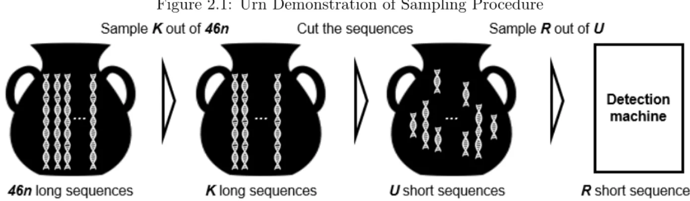
Figure 2.1: Urn Demonstration of Sampling Procedure
Three urn demonstration of the algorithm: the first urn contains raw biological materials; the second urn contains materials sampled from the first urn; the third urn contains materials from the second urn that are cut into shorter segments. Content of the third urn is sampled and assayed in the detection machine.
primary and derived material throughout the process? How best to model the technical errors–such as failure to digest at a site–during the processing of the data as these errors can lead to false positives and negatives? Our goal here is to begin to address these issues by developing a straightforward statistical model and using this model to determine the optimal sampling strategy.
2.3 Statistical Model
In this section, we abstract our sampling procedure into an “urn sampling" model. As DNA is processed through the optical mapping procedure, we imagine the material passing through a series of urns. Assume we have 46 different types of long sequences (i.e. chromosomes), each type has
The first urn contains our original biological material, total of46n long sequences out of whichn
of them contain the target sequence. At the first stage, we sampleK sequences without replacement from the first urn, and put them in the second urn. The second urn will therefore contain a random numberX of target sequences. All of theK long sequences in second urn are cut (a.k.a. nicked and labelled) at random locations according to a Poisson process and placed into the third urn. The third urn will therefore contain a random number of U sequences out of which W are target sequences. The content of the third urn models the biological material prepared for assay in a detection machine. Finally, we sample R smaller sequences without replacement out of the third urn and put them into a detection machine. There will be a random number Y of target sequences processed by the detection machine, and the goal is to assure that for some pre-specified values Qandp, we have the probability of Y ≥Qis at least p. Throughout the experiment, the variables (n, K, R) are in our control and we will find the conditions on them to achieve our goal. In this chapter, we call the long sequence in the second urn which contains the fragment of interest as “target sequence”.
Next we state the following biological assumptions for our modeling 1. The length of target sequence isf.
2. The lengths of long sequences in the first urn are approximately L, hereLmax(f, T).
3. Short sequences in the third urn have lengths approximatelyl, andc≈ Ll.
We proceed by describing the probabilistic parts of our model. The distributions and their expectations are summarized in Table 2.2. There are X target sequences in the second urn. It is straightforward to see X ∼H(46n, n, K), a Hypergeometric distribution with 46n samples, n
samples of interest andK as sampling size.
Let Ui (i = 1,2, .., K) denotes the number of cuts on i-th long sequence in the second urn. Combine with the third assumption above, we assume thatUi follows a Poisson distribution with mean c. Note thatUi cuts divide the sequence into (Ui+ 1) shorter sub-sequences. Consequently,
U =PK
i=1(Ui+ 1) is the total number of short sequences in the third urn, and (U −K) follows Poisson distribution with mean cK.
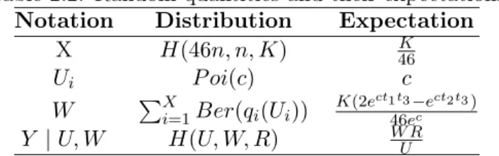
Table 2.2: Random quantities and their expectations Notation Distribution Expectation
X H(46n, n, K) K46
Ui P oi(c) c
W PX
i=1Ber(qi(Ui))
K(2ect1t3−ect2t3) 46ec
Y |U, W H(U, W, R) W RU
sequence contained in the second urn. We haveW =PX
i=1Bi, where fixX,{Bi}Xi=1 are independent
Bernoulli random variables. Condition on {Ui}Ki=1, the probability of success qi of random variable
Bi satisfies the following relation
qi(Ui)
≥2(t1t3)Ui−(t2t3)Ui if T ≥f, =tUi3 otherwise,
(2.1)
wheret1 = LL−−Tf,t2 = L−L2−Tf+f, and t3= 1− fL, respectively. The proof is found in Appendix A.1.
Finally, conditional on U andW, the number of target sequences in the detection machine Y
follows a Hypergeometric distribution with parameters (U, W, R). 2.3.1 Analytical calculations
In this section, we present the analytical results of our statistical modeling. Our goal is to set the sampling parametersK and R so that we can guarantee
P(Y ≥Q)≥p, for pre-specified Qand p. (2.2)
Now we consider Rlow, such that with pre-fixed quantities p0,U andW
P(Y ≥Q|U, W, R≥Rlow)≥p0. (2.3)
Note hereY|U, W ∼H(U, W, R). We will findRlow as a function ofU, W, p0 from tail bounds on
Hypergeometric distribution.
In this chapter, we use the concentration inequality in Lemma A.3.2 on Binomial distribution to control the tail bounds of Hypergeometric distribution. Specifically, we will use the following theorem:
Bb ∼Bin(A−C,BA) be two binomial random variables. Then under conditions on A, B, C and x listed in Appendix A.2, the following inequalities are true
P(h≤x)≤P(Ba≤x), (2.4)
P(h≤x)≤P(Bb ≥B−x). (2.5)
The proof is in Appendix A.2. Numerical results presented in Section 2.5 suggest that for large
C (2.5) is a better bound, in the remaining cases we will use (2.4).
Usually, one would want to fix (A, B, C) and calculate the tail bounds with different x. In this case only Property A.2.1 is needed to ensure the validity of Theorem 2.3.1. The remaining properties proved in Appendix A.2 ensure the validity of Theorem 2.3.1 for the other cases needed in Algorithm 1 when (A, B, C)are changing. In the subsequent calculations, we assume the conditions for Theorem 2.3.1 are met. In particular, we will use large deviation bounds from Lemma A.3.2 on the two Binomial distributions: Bin(R,WU) andBin(U −R,WU) to find Rlow in (2.3).
Write Rlow=Rlow(U, W, p0). Note that U andW are typically unknown. Therefore,Rlow itself is still a random quantity and we need to further find a upper bound for Rlow depending on nand
K, this is denoted by Rˆlow. With large probability, sampling Rˆlow sequences in the third urn is enough to guarantee sampling no less than Rlow samples.
It is fairly straightforward to seeRlow increases withW and decreases withU. Now we fixQand
p0, and writeUupandWlow as the probabilistic upper/lower bounds forU andW, respectively. From (2.4) and (2.5) we can findRˆlow directly from tail bounds onBin(R,WlowUup )andBin(Uup−R,WlowUup ).
In particular, the steps needed to determine Rˆlow for a given K and nare summarized here: 1. Use Lemma A.3.2 on Binomial distributions Bin(K,461) andBin(46n−K,461) to find lower
boundXlow of X. HereXlow depends only onn,K andp1 so that: P(X≥Xlow)≥p1.
2. Set X :=Xlow from step 1. Note thatW is the summation of Xlow independent Bernoulli trials. Hence from Lemma A.3.2 we can find lower boundWlow ofW depending only onn, K,
L, f, T, c, p1, p2 so that:P(W ≥Wlow |X≥Xlow)≥p2.ConsequentlyP(W ≥Wlow)≥p1p2.
4. Use Lemma A.3.2 on binomial distributions Bin(R,WlowUup ) and Bin(Uup−R,WlowUup ) to find
ˆ
Rlow so that
P( ˆRlow ≥Rlow)≥P(U ≤Uup, W ≥Wlow)
≥P(U ≤Uup) +P(W ≥Wlow)−1
=p3+p1p2−1.
Note that we need to ensure the needed sample size R is not larger than the available number of short sequencesU. To this end, both Rˆlow and Ulow are deterministic functions of given constants and we can add numerical constraint onRˆlow to force it smaller thanUlow. A key observation from our numerical result is, as K gets larger, Uup and Ulow will be more concentrated around the mean
cK+K, whileRlow will be much smaller than Ulow. Therefore, we need to find a lower boundKmin on K to ensure Ulow ≥Rˆlow.
Finally, given that we chooseK andRˆlow as our sampling sizes at two stages, respectively. The following relations are true
P(Y ≥Q)≥P(Y ≥Q, R≥Rlow, U ≥R) ≥p0·P( ˆRlow ≥Rlow, U ≥Rˆlow) ≥p0·
h
P( ˆRlow ≥Rlow) +P(U ≥Rˆlow)−1 i
≥p0(2p3+p1p2−2). (2.6)
It suffices to set the desired probability p equal to the right-hand-side of (2.6). The exact selection of {pi}3i=0 can be found in Section 2.4. We will also show in Section 2.4.1 that the range ofK is [Kmin,45n]. While not everyK in this range is feasible, a straightforward monotone analysis shows that as long asK is larger than a certain threshold, the solution Rˆlow always exists.
2.3.2 Optimal sampling strategy
In this section, we discuss how to use the formulas derived in Section 2.3.1 to find the optimal values ofnandK for any givenpand Q. Specifically, assume there is a user-specified cost function
f(·,·)is an monotone increasing function of both nand K. The proposed procedure is summarized here:
1. Solve for{pi}3i=0 such thatp=p0(2p3+p1p2−2).
2. For fixedn, we calculate Kmin.
3. For any fixednand K such thatK ≥Kmin, we calculate Rˆlow. 4. Return: (n, K,Rˆlow).
The implementation details are discussed in Section 2.4. In reality the amount of biological materials is limited, hence there is an upper bound on n and there are only finite number of
(n, K,Rˆlow)to consider. We do not need to consider anyR >Rˆlow as that would lead to sub-optimal design. However, for fixed n, we do need to considerK > Kmin, because largerK might lead to smallerRˆlow and a more efficient solution.
Assume we have a cost function C(K, R) that increases withK andR. We only have finitely many(n, K,Rˆlow) to consider and a brute force search among all the possible triples will yield the optimal (n, K,Rˆlow) minimizing the cost function.
Due to technology limits, we may have certain constraints on sampling percentages: for example, we can only sample 80%in the first stage, and50%from the second stage. We can still use a brute force search only considering the cases that do satisfy these extra constraints.
2.4 Sampling algorithm
In this section we discuss the implementation details of optimal sampling strategy in Section 2.3. The following quantities should be specified/calculated beforehand:
1. Specify the values ofL,f,T,p,Q,n,caccording to the particular application. 2. Select p0 =
√
p,3p3−2 =
√
p andp1=p2:=
√
p3 so that the right-hand-side of (2.6) isp.
3. Compute: t1 = LL−−Tf,t2 = L−L2−Tf+f,t3= 1− fL and set Q1 = 2e
ct1t3−ect2t3
ec ,v=Q1−Q21. Here Q1 and v are the expected value and variance of Bernoulli Ber(qi(Ui))random variable. 2.4.1 Lower bound on K
We need to find the lower bound Kmin ofK such that with large probability we have at least
cutting process in urn 2 does not break any target sequences and we take everything out from urn 3. Therefore, we only need to make sureX is larger than Q with high probability. In Section 2.5, we solved both (2.4) and (2.5) to get different lower bounds for K, similarly with different lower bounds onK we will have different lower bounds for downstream quantities likeX,U etc.
2.4.2 Lower bound on R
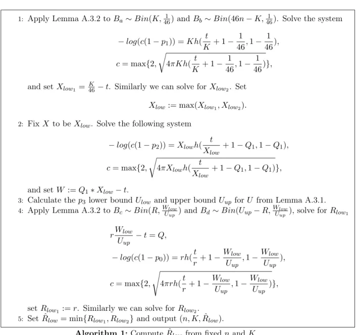
Algorithm 1 can be used to calculate Rˆlow with pre-fixed nandK. Please note, that we use tail bounds of binomial distribution to approximate that of Hypergeometric distribution in step 1, 2 and step 4. Here steps 1 and 2 only require property 1 and 2 in Appendix A.2. Step 4 additionally needs property 3 and 4, because we need the relations in (2.4) and (2.5) to be true with both W ≥Wlow and U ≤Uup. For each fixed n, the range of K is relatively small, thus for each inputn we can simply try all the possible K and calculate the corresponding smallest R (denoted byRlow) that achieves our goal. To make our algorithm more efficient, we can first find the smallestK that can give us a lower tail that is larger thanQ (any smaller K will not be feasible, see our supporting code for details), call thisKmin. For each K from Kmin to 45n, we use Algorithm 1 to findRlow. 2.5 Numerical results
For our numerical results, the calculations were based on biologically reasonable parameters:
L= 250000000,f = 50000,T = 75000,c= 60,p= 0.95,Q= 20.
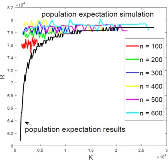
In Figure 2.2, we plot our original calculation results from Algorithm 1 together with the results without using any concentration inequalities (we get the tail points by the inverse of cumulative distribution functions, which is applicable for relatively small n); both of them have the similar patterns. From original calculation results we can find two “kinks” for each fixedn. This is because when K is small, we will need to sample almost everything from the second stage, which will force us to choose the correspond Bin(Uup−R,WlowUup ) for Y as the binomial bounds. Then as K gets larger but not big enough, we will use Bin(R,WlowUup ) for both stages. FinallyK will get close to 45n
which again forces to use Bin(Uup−R,WlowUup ) at the first sampling stage. The performance of our algorithm is slightly more conservative than the concentration inequality free approach in the sense that we ask for more samples. However, each lower bound of our algorithm can be solved efficiently using numerical method, while using inverse cdf function is generally slow for largen.
Figure 2.2: Approximation results of K vsRˆlow
We use Algorithm 1 fornranges from n= 100to n= 600, different colors correspond to different n. Curves at the bottom correspond to concentration inequality free results, while dotted curves at the top correspond to results calculated from our algorithm.
1: Apply Lemma A.3.2 to Ba∼Bin(K,461) and Bb ∼Bin(46n−K,461). Solve the system −log(c(1−p1)) =Kh(
t
K + 1− 1 46,1−
1 46),
c= max{2,
r
4πKh( t
K + 1− 1 46,1−
1 46)},
and setXlow1 =
K
46 −t. Similarly we can solve forXlow2. Set Xlow := max(Xlow1, Xlow2).
2: FixX to be Xlow. Solve the following system −log(c(1−p2)) =Xlowh(
t Xlow
+ 1−Q1,1−Q1),
c= max{2,
r
4πXlowh(
t Xlow
+ 1−Q1,1−Q1)},
and setW :=Q1∗Xlow−t.
3: Calculate thep3 lower bound Ulow and upper boundUup for U from Lemma A.3.1.
4: Apply Lemma A.3.2 to Bc∼Bin(R,WlowUup ) andBd∼Bin(Uup−R,WlowUup ), solve for Rlow1
rWlow Uup
−t=Q,
−log(c(1−p0)) =rh( t r + 1−
Wlow
Uup
,1− Wlow
Uup
),
c= max{2,
s
4πrh(t r + 1−
Wlow
Uup
,1−Wlow
Uup
)},
setRlow1 :=r. Similarly we can solve for Rlow2.
5: SetRˆlow= min{Rlow1, Rlow2} and output(n, K,Rˆlow).
Algorithm 1:Compute Rˆlow from fixedn andK
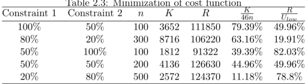
Table 2.3: Minimization of cost function
Constraint1 Constraint2 n K R 46Kn UlowR
100% 50% 100 3652 111850 79.39% 49.96%
80% 20% 300 8716 106220 63.16% 19.91%
50% 100% 100 1812 91322 39.39% 82.03%
50% 50% 200 4136 126630 44.96% 49.96%
20% 80% 500 2572 124370 11.18% 78.8%
as many as possible in the second stage.
We have also applied our algorithm to other choices of Q. The lessons learned are similar to what we have shown here. In the supporting materials we provide Matlab code that can be used to calculate optimal sampling strategy with different parameters.
2.6 Conclusion
In this chapter, we have developed an optimization approach for estimating the amount of material needed for genomic mapping based on a simple, yet realistic, model of the process that uses a novel result regarding the tail bounds of the Hypergeometric distribution. Our approach is both computationally and analytically tractable and we show thatif a genomics mapping technology can sample most of the chromosomal fragments within a sample, comparatively little biological material is needed to detect a variant at high confidence.
CHAPTER 3
Semi-Parametric Model for Optical Mapping
3.1 Introduction
Early optical mapping technologies were limited in scope and scale of the genome that could be assessed. While microbial genomes could be readily assembled, more complex genomes were both technically and algorithmically challenging. A classic tool, Gentig, produced de novo assemblies without requiring an initial estimate of the genome-wide restriction map [Anantharaman et al., 1999], but was limited to small genomes. Other solutions included a heuristic assembler that uses pairwise Smith-Waterman alignment [Shi et al., 2016, Valouev et al., 2006b], subdividing the assembly problem in many smaller problems and using a low-level assembly engine [Mullikin and Ning, 2003]. Other approaches include methods originally developed from plasmid mapping Huddleston and Eichler [2016], Pendleton et al. [2015] and references therein.
potentially indicate a structural variant.
As the molecular technology of optical mapping has matured, the amount of data generated by these technologies has exponentially increased. Algorithms for aligning optical reads have focused on using fast computer science techniques to efficiently align the data. Dynamic programming and de Bruijn graphs, for example, are commonly used in these fast aligners [Valouev et al., 2006c, Luebeck et al., 2020, Fan et al., 2018]. The OMTools suite is an excellent example of these types of tools and provides a comprehensive set of fast algorithms and visualization tools [Leung et al., 2017a].
Optical genome mapping technologies are expected to be used for clinical diagnosis of SV associated with genetic disorders in the near future. In this scenario it is important to assess how well the optical mapping data support the presence of a variant and how well the data support the canonical reference sequence. For example, low confidence in the optical data supporting the reference sequence in a genomic region of interest may motivate further investigation of that region in an affected patient even if a variant is not called. Recognizing this issue, we developed a probabilistic semi-parametric approach for modeling the fit of optical mapping reads to a reference genome. Our approach allows us to assign each optical mapping read to its most likely location in the genome and rigorously assess the credibility of that assignment. Further, by developing an explicit statistical model for these procedures and implemented it as a open-source package, we make transparent both the model’s assumptions and it’s implementation. This work is a critical first step towards building a comprehensive analytical system for using optical mapping and similar data for characterizing structural variation in any genome.
3.2 Approach
DNA sequence of the individual is not known. Instead, a reference genome, such as human Genome hg38, is used or generate the expected pattern of lengths. Again, the observed optical mapping fragment can then be matched to part of the reference array in order to identify the genomic region corresponding to the source of observed fragment. Several possible complications may affect how readily the observed fragment is mapped back to the reference. First, the DNA analyzed may harbor genetic variation causing it to differ from the reference genome. Second, diploid organisms harbor two copies of each chromosome, which may mean that neither regions is an exact match. Third, stochastic shearing of the DNA during the optical mapping may fragment the DNA. This may cause some fragments to be unobserved and will lead to erroneous lengths at the ends of the ordered arrays. Fourth, errors in the nicking or fragmenting process may lead to spurious lengths or missing sites. Finally, complex eukarotic genome are often rich in long arrays of repetitive elements that result in non-unique ordered arrays.
Here, our objective is to identify the “best” position within the genome for a set of observed fragments and provide robust estimate of thequality of the match. We build a statistical model to determine the quality of a position in the genome. In principle, this model could be applied to all fragments produced by an experiment, but the time needed to compute for any large dataset is long. We take advantage of the fact that most of the genome is a terrible fit for any one read. Using some conservative bounds and heuristics, and a rapid filtering algorithm we are able to accelerate the algorithm so that it can be applied to a human sized dataset.
3.3 Methods
In this section we introduce a probabilistic approach in assessing the quality of alignments in optical mapping.
3.3.1 Model Setting
The optical mapping can be modeled through a mapping function from reference genome to observed reads. Specifically, we may write the reference genome as[l1, ..., lN], hereli represents the length (bp) between two adjacent enzyme cutting sites. Similarly we may write the observed reads as
[r1, r2, ..., rm]. We call{ri}mi=1 and {li}Ni=1 fragments and both of them are sets of positive integers.
Figure 3.1: Demonstration of optical mapping.
Demonstration of our method. The reference genome and reads are represented as vectors of positive integers. The filtering algorithm is used to propose the coordinates of candidates sequences. In the bottom part we have one specific read and three candidate sequences correspond to it. The{li}3i=1
are likelihoods calculated from fitted semi-parametric distribution, here we expect l2> l1 l3.
1. Missing signals: enzyme sites get missed.
2. Extra signals: spurious extra enzyme sites appear in the genome.
3. Resolution error: fragments that are shorter than a threshold are not observable. 4. Sizing error: the original fragment and the mapped fragment have different lengths.
At this moment, we do not consider missing signals and extra signals. In Section 3.5, we will show the extension of our model to these two errors. Throughout this chapter, we assume
1. The optical mapping between fragments are completely independent. 2. Cutting happens exactly at the enzyme cutting sites.
3. Fragments generated by optical mapping that are shorter than a constant thresholdT are not observable, this is the resolution error.
means that the dimension of original sequence of [r1, ..., rm] might be larger than m, i.e. short mappings are censored. For a given observed sequence[r1, ..., rm], the likelihood that it was generated from candidate sequence[li1, ..., lik]can be modeled as a posterior probability
P([li1, ..., lik]|[r1, ..., rm])∝P([r1, ..., rm]|[li1, ..., lik])·P([li1, ..., lik]), (3.1)
where{ij}kj=1∈N+ are indexes in[N],m≤k. For the prior part we have
P([li1, ..., lik]) =
∞
X
q=2 λqe−λ
q! ·q(q−1)c
q−2∗L−2
=
λ L
2 ·e
λc
eλ
∞
X
j=0
(λc)je−λc j!
=
λ L
2 ·e
λc
eλ , (3.2)
where q ∼P oi(λ) is the number of total cuttings in the reference genome (conditional on q, the cutting positions are uniformly distributed in[0, L].), and c= L−Le+b (L=PN
i=1li is the physical length of reference genome,bandeare the physical starting and ending positions of[li1, ..., lik]in
the reference genome).
For the likelihood part we have
P([r1, r2, .., rm]|[li1, ..., lik]) =
Πkj=1glij(rj), k=m
0, m > k
P q1,..,qm
h
Πmj=1glqj(rj)·Πj∈I\{q1,..,qm}Plj(x≤T)
i
, m < k, ,
where I ={i1, ..., ik}, andgl(·) is the density function of some unknown distribution that takelas the parameter. Note thatgl(·) catches the sizing error of optical mapping. In next section we will use the semi-parametric approach to model the density function.
3.3.2 Mapping Function via Semi-Parametric Generalized Linear Model
Mathematically speaking, assume fragmentr was generated from fragment l, then
r = (1 +se)l+me, (3.3)
where se is the scaling factor, me is the measurement error. Previous works usually assume se and me are constants throughout ALL fragments. There are at least two issues with this heuristic approach: (1) the fragment lengthsr andl are positive integers, but addingse andme violates this assumption; (2) the parametric approach are inflexible, especially because it assumesse andme are constants. In this chapter, we developed a semi-parametric GLM (SPGLM) model for the density function, which has higher flexibility and can approximate the true probabilistic nature of optical mapping.
Start from the uni-variate exponential density function
f(y|θ) =exp{φ(y) +θy−A(θ)}. (3.4)
In parametric exponential family,φ(y)is a parametric function ofy,A(θ)is the normalizing constant andθ is called the natural parameter. In SPGLM, φ(·) is modeled as a non-parametric function, and θis a linear function of the co-variates X.
Use the same definitions for r andl as above. In stead of modeling the relationship between them as in (3.3), we consider the following standardized discrepancy betweenr and l
y=
√
r−√l
√
l . (3.5)
The standardization in (3.5) allows us to model the density function in a wider domain. Specifically, we model y as a random variable generated from the semi-parametric exponential family in (3.4), where φ(·) is a non-parametric function on the support ofy and θ=β0+β1·x, herex=
√
l. Our goal is to estimate φ(·) and β.
Given a training set {(xi, yi)}in=1, the maximum likelihood estimators ofφ(·) andβ can be found
Constructing Training Set In optical mapping, we only have access to the reference genome and thousands of observed reads. The exact position of original sequence for each observed read is unknown to us and technically impossible to locate with 100% confidence. Consequently, we do not have a “ground truth” training set at hand. In this dissertation, a heuristic minimization algorithm is used to construct the “heuristic training set”.
The average relative error between a observed sequence [r1, .., rm] and a candidate sequence
[li1, ..., lim]is calculated as
E = 1 m
m X
j=1
√
rj−plij p
lij
. (3.6)
Our minimization algorithm takes an observed sequence (i.e. [r1, .., rm]) as input, and output the candidate sequence in the reference genome that delivers the smallest average relative error calculated from (3.6). Note that we only consider candidate sequence with same dimension as the input, i.e.
k=m. To get the training set, we apply the heuristic minimization algorithm to1000reads extracted from real experiments. The sequences that have minimal smallest average relative errors are used to construct the training set. Specifically, we use the fragments in these reads and their corresponding fragments in the reference genome found by the heuristic minimization algorithm as the “ground truth”. Finally we have a sample with3000standardized (see (3.5)) training samples(xi, yi).
Constraints on φ(·) Given a training set{(xi, yi)}in=1. We write{y(i)}ni=1 as the order statistics
of {yi}ni=1 in ascending order. The range[y(1), y(K)]is used as the support of our semi-parametric
distribution, hereK ≤n since we may have duplicates.
In this dissertation, function φ(·) is modeled as a concave piece-wise linear function that only changes its slope at{y(i)}
(K)
i=1. Writeφk=φ(y(k)), then for ∀y∈R we have
φ(y) =
1− y−y(k)
y(k+1)−y(k)
φk+
y−y(k)
y(k+1)−y(k)φk+1, ify ∈[y(k), y(k+1)]
−∞, o.w.
Let∆k=y(k+1)−y(k). To assure the concavity ofφ(·), we need for ∀2≤k≤K−1
− 1
∆k−1
φk−1+
1 ∆k−1
+ 1
∆k
φk−
1 ∆k
Writeα=B·φ, where B=
1 − 1
∆1 0 · · · 0
− 1
∆1 · · · 0 . . . .
· · · − 1 ∆i−1
1 ∆i−1 +
1
∆i −
1 ∆i · · ·
. . . .
0 · · · ∆1 K−1 1
.
The concavity constraint can be rewritten: αk≥0 for k= 2, .., K−1.
To make our estimation identifiable, we also add the following identifiability constraints
Z y(K)
y(1)
eφ(y)dy= 1,
Z y(K)
y(1)
yeφ(y)dy= 1. (3.8)
See [Zhang, 2017, Chapter 4] for a detailed discussion on why these constraints are needed and why they work. The numerical set up of these constraints is discussed in Section B.1.
3.3.3 Optimization with Projected Gradient Descent Algorithm
To find the MLE of φ(·)and β, we want to maximize the following objective function
Ln(φ, β) = ΠNi=1exp{θiyi+φ(yi)−A(θi)}, (3.9)
where
A(θi) = log Z y(K)
y(1)
eθiy+φ(y)dy.
Note thatLn(φ, β) is the likelihood function of SPGLM. We solve the optimization problem in a projected gradient descent fashion, i.e. we first do the steepest descend on φ, and then project it back to the feasible region, then do the same procedure for β, we iterate these two procedures until the results converge. Handling identifiability modification is tricky, we leave the technical details in Appendix B.1.
1. Initializeβ andφ.
2. Fixing φˆ, updateβˆ by doing gradient descent with respect to
ln(β) = n X
i=1
{xTi βyi+ ˆφ(yi)−log K X
k=1
exp( ˆφk+xTi βyk)}. (3.10)
3. Fixing βˆ, update φˆby doing gradient descent with respect to
ln(φ) = n X
i=1
{xTi βyˆ i+φ(yi)−log K X
k=1
exp(φk+xTi βyˆ k)}. (3.11)
4. Update φˆby projecting it back into the feasible region. 5. Iterate over Step B to StepD until convergence. 6. Modify φˆby the following equation
ˆ
φ:= ˆφ+θ∗y−log
Z ∞
0
eφˆ+θ∗ydy. (3.12)
Hereθ∗ satisfies the following condition Ry(K)
y(1) ye ˆ
φ+θ∗y
dy
Ry(K) y(1) e
ˆ
φ+θ∗y
dy = 1.
We can use binary search to numerically solve forθ∗. It is fairly straightforward to check this modification can actually meet the identifiability constraints in (3.8).
The closed formulas needed for optimization are presented in Appendix B.1. The implementation details can be found in supplementary codes.
3.3.4 A Boolean-Matrix-based Filtering Algorithm
Generally speaking, any subsequence [li1, ..., lik]of the reference genome wherek≥m could be a
The filtering algorithm starts with a boolean matrix (matrix with only1’s and 0’s as its entries)
B∈Rm×N such that
Bij =
1, if
√
ri√−√lj
lj ∈[y(1), y(K)].
0, otherwise.
In words, Bij = 1 if and only if it is feasible that lj to map into ri. If no drops are allowed, a sequence[li1, .., lim]is a feasible potential original sequence if and only if Π
m
j=1Bj,ij = 1. Under the semi-parametric distribution, a fragment lij can be dropped if and only if
√
T−p
lij p
lij
∈[y(1), y(K)]. (3.13)
Therefore we can pre-calculate a vector v∈RN such that
vj =
1, if (3.13) is satisfied.
0, otherwise.
(3.14)
Vector v stores the set of fragment indexes that can be dropped.
Definition 3.3.1. A sequence [li1, ..., lik] is a feasible candidate with respect to read [r1, ..., rm] if
and only if: there exists a subset{s1, s2, ..., sm} of [i1, .., ik] such that
Πmj=1Bj,sj ·Πi∈[i1,..,ik]\{s1,...,im}vi = 1.
We call the number of drops allowed as the dropping threshold. The filtering algorithm takes one read and a dropping thresholddas the input, and outputs all the feasible candidates with dimension
k=m+d. The detailed steps of the filtering algorithm are listed in Algorithm 2. Please note that in Step3,j is not a positive integer, instead it is a tuple that contains one possible combination of dropping positions. For example, when k=m+ 1, the dropping position could happen at any position between 2andm (we do not consider the first dimension nor the last dimension, since it essentially degenerates to the casek=m), soj is a list that contains just one positive integer; when
input: The reference genome L, the observed read[r1, ..., rm], the dropping threshold d, the corresponding boolean matrixB, and the dropping index vectorv.
output: The matrixCthat stores the starting and ending positions for all feasible candidates.
1. CalculateJ as the set that contains all the combinations of possible positions of drops, so the cardinality ofJ is m+dd−2
. 2. forj∈ J do
for i= 1 toN −m−d+ 1do
[j1, ..., jm] :={i, i+ 1, ..., i+m+d−1} \(i+j) if Πm
s=1Bs,jsΠt∈jvt== 1 then
C= [C;i, i+m+d−1]
end end end
Algorithm 2:Boolean Matrix Based Filtering
Pre-filtering of reference genome One drawback of Algorithm 2 is, the dropping thresholdd
is prefixed. This limits our searching space in the whole reference genome. One solution to this issue is to try differentd and merge the outputs. While it is relatively cheap to run Algorithm 2 with smalld, the cardinality ofJ in Algorithm 2 makes largedprohibitive. In this section, we discuss the pre-filtering of reference genome, which can significantly increase the searching space of Algorithm 2.
To pre-filter the reference genome, we remove all the fragments in the reference genome with lengths smaller than a thresholdc(T). For any specific original sequence, we can divide its fragments into three categories: (1) fragments that map into the observable reads, hence the number of fragments in this category equals to the dimension of observed read, (2) fragments that are shorter thanc(T)and map into something un-observable, (3) fragments that are longer than c(T)and map into something un-observable.
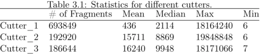
Table 3.1: Statistics for different cutters.
# of Fragments Mean Median Max Min Cutter_1 693849 436 2114 18164240 6 Cutter_2 192920 15711 8869 19848848 6 Cutter_3 186644 16240 9948 18171066 7
drops and add flexibility to the algorithm. Definec(T)p as a constant such that
P "
x≤ p
c(T)p− √
T
p
c(T)p #
≤1−p. (3.15)
Therefore c(T)p is monotonically increasing inp. WriteLp as the vector after removing all the frag-ments{li}i∈[N],li<c(T) in reference genomeL, we callLp the “filtered genome”. Applying Algorithm 2 on Lp with different pyields faster calculation since we only need to build boolean matrixB on a shorter vector.
To sum up. In order to avoid narrowing down the searching space of Algorithm 2, we recommend applying Algorithm 2 onLp with different choices of(p, d) and merge all the candidate sequences output by different parameters.
3.4 Numerical Results
In this section, we present our numerical results in two experiments with synthetic optical reads. In the first experiment, we test the performance of our algorithm on a human reference genome with different enzyme cutters. In the second experiment, we compare our algorithm with OMBlast on synthetic reads generated from E.Coli reference genome.
3.4.1 Generating Synthetic Reads
To test the performance of our method, three reference genomes were generated by applying three different cutters on the same human reference genome. In Table 3.1 we summarize the statistics over the lengths of fragments correspond to each cutter. Since the cutters are used on the same human genome, all of these genomes have same lengths and larger number of fragments means more short fragments.
For each cutter, we randomly sample 1000 original sequences from it. The physical length of each sampled sequence is determined based on the lengths of our true optical reads.
each cutter. To be specific, we model the relative error by(1) Negative binomial with p= 0.5,(2)
Normal distribution withµ= 0 and σ= 0.1,(3)semi-parametric distribution we fitted. 3.4.2 Details of Implementation
In this section, we discuss the details of our implementation of SPGLM and the filtering algorithm.
Phase 1: Filtering Algorithm In Phase 1, we setT = 400. This number is determined by the true nature of Bionano optical mapping device. Recall that we want to apply Algorithm 2 on Lp with different (p, d). In our experiments, we pick d= 1,2,3 andp∈[0.11,1](this corresponds to
c(T)p∈[40,600]).
Phase 2: Calculating Posterior In Phase 2, we set the mean of the poisson cutting procedure
λ= PN
i=1li
250000, here 250000 is the average physical length of optical reads and is determined by the
Bionano optical mapping device. Note thatλonly affects the prior.
To speed up the calculation of likelihood function, we use a lower bound of the posterior probability to approximate the full posterior. Specifically, we observed the fact that in real experiments, the true alignment in
X
q1,..,qm
h
Πmj=1glqj(rj)·Πj∈I\{q1,..,qm}Plj(x≤T)
i
usually dominates all the other possibilities. To this end, for each candidate sequence [li1, ..., lik], we
use a dynamic programming approach to find the set{qˆi}mi=1 such that
{qˆi}mi=1= arg min
{qi}m
i=1∈I={i}ki=1
m X
i=1
√
ri− p
lqi p
lqi
.
The term Πmj=1glqjˆ (rj)·Πj∈I\{qiˆ}mi=1Plj(x ≤T) is then used to approximate the likelihood part of
the posterior. We can summarize our implementation by the following steps
1. Pick a set{ptj}sj=1, andd= 1,2,3.
2. For everyptj ∈ {ptj}sj=1, getLptj fromL based on c(T)ptj. 3. Calculate vectorv from (3.14) based onLptj.
5. Implement Algorithm 2 with dropping thresholdd, filtered reference genomeLptj, optical read
r, and vectorv. Assume we get candidate set Cptj,d. 6. Merge the candidate setsC=∪s
j=1Cptj,d. 7. Calculate the posterior of every candidate inC.
Results on Synthetic Reads from Human Reference Genome After Phase2, we can rank the candidate sequences according to their corresponding posterior likelihoods. Each candidate sequence can be uniquely identified by its starting and ending positions in the reference genome (not the filtered reference genome). For any two sequences with starting and ending positions(s1, e1)and (s2, e2), we use |s1−s2|+|e1−e2| to measure the physical distance between them. Since we are
doing numerical analysis on synthetic data, the exact starting and ending positions of each original sequence are known to us. Therefore, for each read, we can calculate the physical distances between its corresponding original sequence and the candidate sequences found by the algorithm. We call the candidate sequence that has the smallest physical distance with the original sequence as the “closest match”.
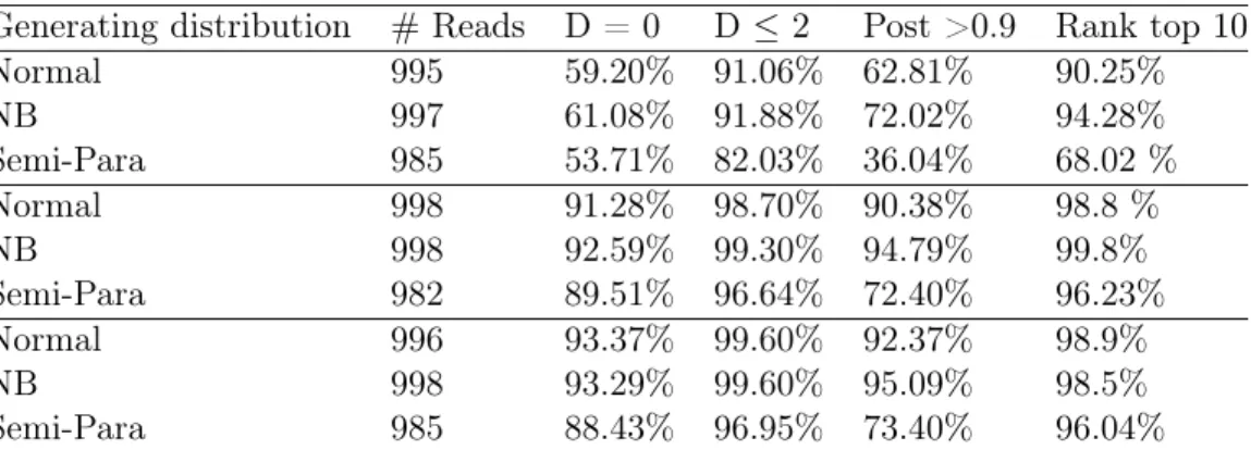
The numerical results is summarized in Table 3.2. Due to the space limitation, we use short names for each column. The corresponding descriptions of columns are under the table. Two desired properties regarding the closest match are
1. The distance between closest match and the true original sequence is small. In Table 3.2 we use “D” to denote this distance, note D is non-negative. A small D means our algorithm finds a candidate close to the truth.
2. The posterior likelihood of closest match is large. Note that even if closest match is the original sequence, to actually pick it out from large amount of candidates, we are more likely to pick it if it is inside some confidence region. In Table 3.2 we use “Post” to denote its posterior likelihood. Alternatively, we want the closest match to have high rank among candidate sequences. This is represented by the third column in Table 3.2, which demonstrates the portion of closest matches that rank top 10among the candidates.
Table 3.2: Results on human reference genome
Generating distribution #Reads D = 0 D ≤2 Post >0.9 Rank top10
Normal 995 59.20% 91.06% 62.81% 90.25%
NB 997 61.08% 91.88% 72.02% 94.28%
Semi-Para 985 53.71% 82.03% 36.04% 68.02 %
Normal 998 91.28% 98.70% 90.38% 98.8 %
NB 998 92.59% 99.30% 94.79% 99.8%
Semi-Para 982 89.51% 96.64% 72.40% 96.23%
Normal 996 93.37% 99.60% 92.37% 98.9%
NB 998 93.29% 99.60% 95.09% 98.5%
Semi-Para 985 88.43% 96.95% 73.40% 96.04%
Each block corresponds to the same reference genome cut by a specific enzyme cutter. For each genome, three different random mechanisms are used to generate the observed reads. In the second column, we record the number of outputs for each category (due to running time limit, we did not get the results for some reads). The third and fourth columns record the percentage of cases where the closest match is close to the true original sequences. The fifth column is the percentage of cases where closest match has a posterior likelihood larger than 0.9. The last column is the percentage of cases where closest match has a posterior likelihood rank top10 among all candidate sequences.
algorithm does not take into account the structural variant at this moment, we can potentially use it for data with structural variant as well.
Comparison with OMBlast Mapping Tool In this section, we compare the performance of our algorithm with another state-of-the-art mapping tool called OMBlast [Leung et al., 2017b] on the synthetic datasets generated from Escherichia coli reference genome.
Specifically, we generated synthetic reads from two different types of data generation mechanisms. The first type is from OMBlast’s data generator, where sizing error is decomposed into scaling error and measurement error. Note that OMBlast is capable of handling missing and extra signals, which is not supported by our algorithm at this moment. Therefore in the simulation we disabled the generation of missing and extra signals. The second type is the same as the previous section, where sizing error is modeled through relative error in (3.5). Similar as before, we generate the relative error based on three different generating distributions. We also added backward reads to make fair comparisons.
The results are summarized in Table 3.3. To decide the direction of mapping from our algorithm, for each specific read [r1, .., rm] we run our algorithm on both [r1, .., rm] and [rm, .., r1]. The
Table 3.3: Comparison with OMBlast
Generating mechanism #Reads Semi Strong Semi Weak Semi All OMB All
OMB 2995 95.53% 0.03% 95.56% 97.83%
Semi-Para 3000 84.53% 0.3% 84.83% 9.1%
Normal 3000 92.4% 0.03% 92.43% 34.03%
NB 3000 94.47% 0.07% 94.53% 90.33%
The first column records the data generation mechanisms, where first raw comes from data generator of OMBlast, second to fourth rows come from relative error with different generating distributions. The second column records the number of synthetic reads under different mechanisms. The third column records the cases where our algorithm find the true original sequences among the top 10
candidate sequences, while the fourth column records the cases where our algorithm finds the true original sequence but the direction is incorrect. The fifth column is the sum of the third and fourth columns. The last column records the percentages of cases where OMBlast successfully find the original sequences.
Note that OMBlast occasionally output the partial alignments. In Table 3.3, we deemed that OMBlast successfully finds the original sequence if and only if: (1) the partial alignment has overlapping with true original sequence, (2) at least half of the read is correctly mapped back to the original sequence.
From Table 3.3 we can see that our algorithm performs consistently well across different generating mechanisms, while OMBlast performs very poorly with medium to large sizing errors. The biggest advantage of our approach over OMBlast is, once the semi-parametric distribution is fitted from data, we do not need to specify any hyper-parameters. While one needs to specify the parameters for OMBlast that controls its tolerance to sizing error.
3.5 Extension to Other Mapping Tools
In this section, we extend the likelihood function in (3.1) to account for missing/extra signals. From this extension, we could potentially stack our semi-parametric likelihood model and other filtering algorithms ( OMBlast Leung et al. [2017b], TWINS Muggli et al. [2014], SOMA Nagarajan et al. [2008] etc.) together.
We start from the following assumptions
1. Each enzyme site has independent chance of missing, the probability of missing is pm. 2. The number of extra signals in a sequence with length Pk
j=1lij follows a Poisson distribution
3. The number of missing signals and extra signals are known to us. The sequence[li1, li2, ..., lik]
is observed AFTER we remove the missing sites and add the extra sites.
Now for observed read [r1, ..., rm] and candidate sequence[li1, li2, ..., lik], write nm andne as the
number of missing/extra signals, andtl=Pkj=1lij. We then have
P([li1, ..., lik])∝
λ L
eλc eλ
pm
1−pm nm
(λetl)nee−λetl
ne!
. (3.16)
Here we add missing/extra signals by Bernoulli trials and Poisson distribution.
In reality, we only have access to Lbefore removing the missing signals and adding extra signals, which is the opposite of Assumption C above. However, alignment tools like OMBlast is able to infer the missing and extra signals. Specifically, OMBlast outputs the sequence[li1, ..., lik]together
with the inferred positions of missing/extra signals. From these information, we can directly get the candidate sequence after add missing/extra signal errors, this is our Assumption C.
CHAPTER 4
Subspace Clustering through Sub-Clusters
4.1 Introduction
In data analysis, researchers are often given data sets with large volume and high dimensionality. To reduce the computational complexity arising in these settings, researchers resort to dimension reduction techniques. To this end, traditional methods like PCA [Hotelling, 1933] use few principal components to represent the original data set; factor analysis [Cattell, 1952] seeks to get linear combinations of latent factors; subsequent works of PCA include kernel PCA [Schölkopf et al., 1998], generalized PCA [Vidal et al., 2005]; manifold learning [Belkin and Niyogi, 2003] assumes data points collected from a high dimensional ambient space lie around a low dimensional manifold, and muli-manifold learning [Liu et al., 2011] considers the setting of a mixture of manifolds. In this dissertation, we focus on one of the simplest manifold, a subspace, and consider the subspace clustering problem. Specifically, we approximate the original dataset as an union of subspaces. Representing the data as a union of subspaces allows for more computationally efficient downstream analysis on various problems such as motion segmentation [Elhamifar and Vidal, 2009], handwritten digits recognition [You et al., 2016a], and image compression [Hong et al., 2006].
4.1.1 Related Work
are then used to cluster the data points. One of the main drawbacks of SSC and DSC is their computational complexity of O(N2) in both time and space, which limits its application to large datasets. To address this limitation, a variety of methods have been proposed to avoid solving complicated optimization problems in constructing the affinity matrix. Heckel and Bölcskei [2015] used inner products with thresholding (TSC) to calculate the affinity between each pair of points, Park et al. [2014] used a greedy algorithm to find for each point the linear space spanned by its neighbors, similarly Dyer et al. [2013] and You et al. [2016c] used orthogonal matching pursuit (OMP), You et al. [2016b] used elastic the net for subspace clustering (ENSC) and proposed an efficient solver by active set method. However, these methods require running spectral clustering on the fullN ×N affinity matrix. A Bayesian mixture model was proposed for subspace clustering in Thomas et al. [2014], but its parameter inference is not scalable to large dataset. Zhou et al. [2018] used a deep learning based method which does not have theoretical guarantee.
Recently, there have been two methods that increase the scalability of sparse subspace clustering. The SSSC algorithm and its varieties [Peng et al., 2016] clusters a random subset of the whole dataset and then uses this clustering to classify or label the out-of-sample data points. This method scales well when the random subset is small, however a great deal of information is discarded as only the information in the subset is used. In You et al. [2016a] a divide and conquer strategy is used for SSC—the data set is split into several small subsets on which SSC is run, and clustering results are merged. This method cannot reduce the computational complexity of the SSC by an order of magnitude so is limited in its ability to scale to large dataset.
4.1.2 Contribution
deliver better clustering results.
We provide theoretical guarantees for our procedure in Section 4.3. The analysis reveals that under mild conditions, the subspaces can share arbitrarily many intersections as long as most of their principal angles are larger than a certain threshold. While our algorithm for finding neighboring points is similar to that of Heckel and Bölcskei [2015], the data generation model and assumptions underlying our theorems are different–we take into account the fact that after normalization the noisy terms will no longer follow a multivariate normal distribution. While our work is originally designed for linear subspace clustering problems. The idea of clustering through sub-clusters can be easily extended our to general clustering problems. See our discussion in Section 4.2.1.
We apply our algorithm to both synthetic and real world datasets. The experimental results demonstrate that our method is highly scalable and can deliver superior accuracy compared to other state-of-the-art methods.
4.1.3 Chapter Organization
The rest of this chapter is organized as follows: in Section 4.2, we describe the model setting and the implementation of our clustering procedure, in Section 4.3 we state theoretical guarantees for our procedure and explain in some details the geometric and distributional intuitions underlying our procedure. The detailed proofs can be found in Appendix C.1, in Section 4.4 we present experiments on four datasets and compare our method with state-of-the-art methods, a comprehensive report of the numerical results can be found in Appendix C.3.
4.1.4 Notation
Throughout this chapter, unless specified otherwise, we use capital bold letter to denote data matrix, and corresponding lower bold letter to denote the columns of it. In this chapter, we are given a dataset Y with N data points in RD. Writeyi as the i-th column ofY, andY−i is the matrix
Y with the i-th column removed. Similarly, we write y−j as vectorywith the j-th entry removed. The complement of event E is denoted byE{. We use subscript with parenthesis to represent the
order statistics of entries in a vector, for examplea(i) is thei-th smallest entry in vector a, while
without ambiguity both a(i) and ai refer to the i-th element of vectora. The unit sphere in Rd is denoted bySd−1. We assume each data point of Y concentrates near exactly one of K linear subspaces denoted by{Sk}K