IOS Press
A single and double mode approach to
chaotic vibrations of a cylindrical shell with
large deflection
Liming Dai
a,∗, Qiang Han
band Mingzhe Dong
caIndustrial Systems Engineering, University of Regina, 3737 Wascana Parkway, Regina, Saskatchewan, Canada
S4S0A2
bDepartment of Mechanics, College of Traffic and Communications, South China University of Technology,
Guangzhou, China 510640
cPetroleum Systems Engineering, University of Regina, 3737 Wascana Parkway, Regina, Saskatchewan, Canada
S4S0A2
Received 13 October 2003 Revised 8 December 2003
Abstract. The chaotic vibrations of a cylindrical shell of large deflection subjected to two-dimensional exertions are studied in
the present research. The dynamic nonlinear governing equations of the cylindrical shell are derived on the basis of single and double mode models established. Two different types of nonlinear dynamic equations are obtained with varying dimensions and loading parameters. The criteria for chaos are determined via Melnikov function for the single mode model. The chaotic motion of the cylindrical shell is investigated and the comparison between the single and double mode models is carried out. Results of the research show that the single mode method usually used may lead to incorrect conclusions under certain conditions. Double mode or higher order mode methods should be used in these cases.
Keywords: Galerkin principle, melnikov function, chaos, nonlinear dynamics, cylindrical shell, single and double mode methods, numerical analysis
1. Introduction
In recent years, chaos in nonlinear dynamic systems has aroused more and more interest in the field of theoretical and experimental mechanics. Chaotic motion is regarded as a natural extension of the study object in nonlinear vibration. In solid mechanics, the chaotic behavior of buckled beams is studied by numerous researchers [1–4], and motion of the beams has been well understood. Among the recent research, the periodic and chaotic behavior of a viscoelastic nonlinear bar subjected to harmonic excitations was investigated by Suire et al. [5] on the based of a dynamics model established with implementation of Galerkin principle. The periodic and chaotic response of a slender beam with an attached mass under vertical base excitation was also reported [6]. However, a significantly less number of archival publications is available in investigating the chaotic properties of plates and shells. The forced response of a nearly square plate, the nonlinear dynamics of a shallow arch, and the chaotic motion of a circular plate and a cylindrical shell are a few typical studies in mechanical and structural systems found in the research [7–9]. Moreover, the single mode method is usually employed in the analysis of nonlinear dynamic systems. A typical
∗Corresponding author. E-mail: [email protected].
L
2R
o
x
x
Q
x
Q
r
Q
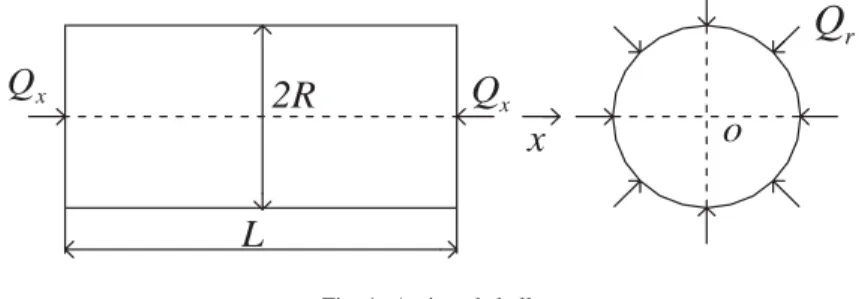
Fig. 1. A pinned shell.
example can be found from the article by Moon [2]. This article significantly contributes to the chaotic response of an elastic beam subjected to a periodic excitation with nonlinear boundary conditions and provided the criterion for chaos on the basis of a single mode model. In fact, most of the studies on nonlinear behavior of elastic elements utilize the single mode method. Based on the current literature, the differences between the single and double or higher mode methods have not been attended.
Cylindrical shells are widely used in civil, mechanical and petroleum engineering practices. However, a compre-hensive understanding of the nonlinear behavior of the shells under dynamical loading is far from being reached. Among the available publications, for instance, a systematical and thorough study on elastic cylindrical shells of large deflection subjected to multi-axial exertions has not been found. The goal of the present research is to investigate the nonlinear behavior of an elastic cylindrical shell under excitations in longitudinal and radial directions. Large deflection of the shell is to be taken into consideration. Equations of motion for the cylindrical shell will be derived with both single and double modes. Nonlinear behavior of the shell, such as chaos, will be studied. The criteria for chaos of the cylindrical shell will be developed and the chaotic behavior of the transverse vibration of the shell will be investigated through a numerical analysis by the P-T method [10]. Results generated by single and double mode models will be compared and the differences of the two models will be identified and analyzed.
2. Governing equations
A pinned elastic cylindrical shell as shown in Fig. 1 will be studied. The cylindrical shell has diameter2R, thickness
hand lengthLand is subjected to uniformly distributed harmonic excitations,QxandQr, in the longitudinal and radial directions respectively.
The excitationsQxandQrare expressed in the following form:
Qx=qx+qx0cosωxt, Qr=qr+qr0cosωrt (1)
The dynamic equation of the shell with large deflection can then be given in the following form with utilization of von Karman’s theory for large deflection of shells [11].
L(W, t) =D∇4W− 1
R
∂2ϕ
∂x2 −
∂2ϕ
∂x2 ·
∂2W
∂y2 + 2·
∂2ϕ
∂x∂y ·
∂2W
∂x∂y −
∂2ϕ
∂y2 −
∂2ϕ
∂y2 ·
∂2W
∂x2 +ρh
∂2W
∂t2
(2a)
+c∂2W
∂t2 +c
∂W
∂t −Qr= 0
∇4ϕ=Eh∂2W
∂x∂y
2
−∂2W
∂x2 ·
∂2W
∂y2 −
1
R
∂2W
∂x2
(2b) where
D= Eh
3
∇4= ∂4
∂x4 + 2
∂4
∂x2∂y2+
∂4
∂y4 (3b)
In Eqs (2a) and (2b),W denotes the radial displacement,ρthe density of the material,cthe damping coefficient,
µthe Poisson ratio of the material,Ethe elastic constant andϕthe stress function which gives the in-plane forces as follows.
Nx= ∂
2ϕ
∂y2, Ny =
∂2ϕ
∂x2, Nxy=−
∂2ϕ
∂x∂y (4)
Following the Ritz method with two modes, one may have
W(x, y, t) =W1(t) sinπx
L sin
πy
R +W2(t) sin
2πx
L sin
πy
R =W1sinαxsinβy+W2sin 2αxsinβy (5)
where
α= π
L, β=
π
R (6)
Trigonometric mode function is widely employed in describing the motion of a shell or plate [12]. Selection of the trigonometric mode function in the present research is based the consideration of the convenience of the functions in theoretical analysis for the response of the shell under the uniform loadings.
Substitution of Eq. (5) into Eq. (2b) gives
∇4ϕ=Eh(W
1αβcosαxcosβy+ 2W2αβcos 2αxcosβy)2−(−W1α2sinαxsinβy
−4W2α2sin 2αxsinβy)·(−W1β2sinαxsinβy−W2β2sin 2αxsinβy)
−1
R(−W1α
2sinαxsinβ−4W
2α2sin 2αxsinβ)
(7)
=Eh
1
2α2β2W12(cos 2αx+ cos 2βy) +
1
4α2β2W1W2(−cosαx+ 9 cos 3αx+ 9 cosαxcos 2βy
−cos 3αxcos 2βy)+2α2β2W22(cos 4αx+ cos 2βy)+α
2
R(W1sinαxsinβy+ 4W2sin 2αxsinβy)
The stress functionϕcan be obtained as follows
ϕ=Eh
1
2α2β2W12(A1cos 2αx+A2cos 2βy) +14α2β2W1W2(A3cosαx+A4cos 3αx
+A5cosαxcos 2βy+A6cos 3αxcos 2βy+ 2α2β2W22(A7cos 4αx+A8cos 2βy) (8)
+α2
R(A9W1sinαxsinβy+A10W2sin 2αxsinβy)
+y2
2Qx
where
A1=161α4, A2= 161β4, A3=−α14, A4=9α14, A5= (α2+49β2)2
A6=−(9α2+41β2)2, A7= 2561α4, A8= 161β4, A9= (α2+1β2)2
A10=(4α2+1β2)2
(9)
Define the following shorthand notations:
B1= Eh2 α2β2A1, B2= Eh2 α2β2A2, B3=Eh4 α2β2A3, B4= Eh4 α2β2A4
B5= Eh4 α2β2A5, B6= Eh4 α2β2A6, B7= 2Ehα2β2A7, B8= 2Ehα2β2A8
B9= EhR α2A9, B10= EhRα2A10
(10)
ϕ=W12(B1cos 2αx+B2cos 2βy) +W1W2(B3cosαx+B4cos 3αx+B5cosαxcos 2βy
+B6cos 3αxcos 2βy) +W22(B7cos 4αx+B8cos 2βy) +B9W1sinαxsinβy (11)
+B10W2sin 2αxsinβy+y
2
2Qx
Substituting Eqs (5) and (11) into Eq. (2a), one may have
L(W) =D[W1(α2+β2)2sinαxsinβy+W2(4α2+β2)2sin 2αxsinβy]−[W12(−B1·4α2·cos 2αx)
+W1W2(−B3α2cosαx−B4·9α2cos 3αx−B5α2cosαxcos 2βy−B6·9α2cos 3αxcos 2βy)
+W22·(−B7·16α2cos 4αx)−W1B9·α2sinαxsinβy−W2·B10·4α2sin 2αxsinβ]
·
1
R+ (−W1β
2sinαx·sinβy−W
1β2sin 2αxsinβy)
+ 2[W1W2(B5·2αβsinαxsin 2βy
+B6·6αβsin 3βxsin 2βy) +W1B9·αβcosαxcosβy+W2·B10·2αβcos 2αxcosβy]
(12)
·[W1αβcosαxcosβy+W22αβcos 2αxcosβ]−[W12(−B2·4β2cos 2βy)
+W1W2(−B5·4β2cosαxcos 2βy−B6·4β2cos 3βxcos 2βy) +W22(−B8·4β2cos 2βy)
−W1B9sinαxsinβy−W2B10β2sin 2αxsinβy+Qx]·[−W1α2sinαxsinβy
−W2·4α2sin 2αxsinβy] +ρh( ¨W1sinαxsinβy+ ¨W2sin 2αxsinβy)
+c( ˙W1sinαxsinβy+ ˙W2sin 2αxsinβy)−Qr= 0
Employing the Galerkin principle
L(W) sinαxsinβydxdy = 0
L(W) sin 2αxsinβydxdy= 0, (13)
the following nonlinear modal equations can be obtained.
˙
W1+m1W˙1+m2W13+m3W12+m4W1W22+m5W1+m6W1+m7W22+m8= 0
¨
W2+n1W˙2+n2W23+n3W2W12+n4W2W1+n5W2+n6W2= 0 (14)
where
m1=ρhc , m2=2αρh2β2(B1+B2), m3=−3π322ρhRα2 (2B1+β2B9R)
m4=α42ρhβ2(18B4−B6−2B3+ 9B5+ 8B8), m5= ρhR1 (α2B9+D(α2+β2)2)
m6=α2ρhQx, m7=−12815 π2αρhR2 (2B7+ 3β2B10R), m8=−16π2Qrρh
n1=ρhc , n2= 8αρh2β2(B7+B8), n3=α42ρhβ2(32B2+ 18B4−B6+ 9B5−2B3)
n4=−180πα22ρhR(−3456B6+ 4608β2B9R+ 640B5+ 10368B4+ 4608β2B10R−1920B3)
n5=ρhR1 (Dβ4R+ 16Dα4R+ 8Dα2β2R+ 4α2B10), n6= 4αρh2Qx
(15)
LetW1=c1x1, W2=c2x2, t=c0τ, m5c20= 1, m2c20c21= 1, n2c20c22= 1, Eq. (14) can be written as
¨
x1+√m1m5x˙1+x31+
√m3
√m2m5x21+m4n2x1x22+x1+m6m5x1+m7n2
m2
m5x22+m8m5
m2
m5 = 0
¨
3. Melnikov function for the single mode motion
From Eq. (16), the following nonlinear dynamic equation can be constructed if only one mode is considered.
¨
x+√m1
m5x˙+x
3+√m3
m2m5x
2+x+m6
m5x+
m8
m5
m2
m5 = 0 (17)
Two cases are studied using the following common parameters.
L= 0.5 m, R= 0.1 m, h= 0.002 m, α= πL m−1, β= πRm−1
E= 69.7×10⁹Pa, ρ= 2.78×10³kg/m3, µ= 0.3, c= 1.67×10⁷kg·(m2·s)−1
qx= 0, qr0= 0, qr=g×1.56×10¹⁰N/m2
(18)
In the first case,qx0=−106N/m, and Eq. (17) takes the following form
¨
x+ 0.5x−3.8x2+x3=g∗cosωτ−0.82 ˙x (19)
which in general can be expressed as
¨
x+x+αx2+βx3=ε(gcosωt−µx˙) (20)
whereα, β, andεare system parameters.
In the second case,qx0=−4×10⁶N/m, and Eq. (17) reads
¨
x−x−3.8x2+x3=g∗cosωτ−0.82 ˙x (21)
The corresponding general form of this system is
¨
x−x+λ2x2+λ3x3=ε(gcosωt−µx˙) (22)
a) The Melnikov function of Eq. (20)
Whenε= 0, the corresponding unperturbed system is
˙
x=y
˙
y=−x−αx2−βx3 (23)
Its Hamilton function can be expressed as
H(x, y) = 12y2+21x2+α3x3+β
4
4 x4 (24)
The three fixed points are (0,0) and ((−α± α2−4β)/2β,0). For the homoclinic orbit of the system,
x0(t), y0(t))T, the Melnikov function [13] is defined as follows.
M(t0) =
+∞
−∞ y0
(t){−µy0(t) +gcos[ω(t+t0)]}dt=−µA+gB(t0) (25)
where
A=
+∞
−∞ y
2
0(t)dt (26)
B(t0) =
+∞
−∞ y0
(t) cos[ω(t+t0)]dt=
B12+B22cos[ω(t+τ0)] (27)
B1=
+∞
−∞
y0(t) cosωtdt, B2=
+∞
−∞
y0(t) sinωtdt, τ0= arctan(B2/B1). (28)
One may therefore obtain
M(t0) =−µA+g
The homoclinic orbitx0(t), y0(t))T can be determined by using the following equation
H(x0, y0) = 1
2y2+
1
2x2+
α
3x3+
β
4x4 (30)
where(x0, y0)T is the saddle point, and we have
dt/dx=±N−1 (31)
where
N=
2H−x2−2α
3 x3−
β
2x4, H=H(x0, y0). (32)
With these equations,A,B1andB2can be determined as
|A|=
+∞
−∞ y
2 0(t)dt
= 2
x(+∞)
x(0) N dx
, |B1|=
+∞
−∞ y0
(t) cosωtdt= 0 (33)
|B2|=
+∞
−∞ y0
(t) sinωtdt= 2
x(+∞)
x(0)
sin(ω
x
x(0)N
−1ds)dx
(34)
When the Melnikov function has simple zero points, the stable and unstable manifolds intersect. The Poincare map has a horseshoes; there therefore exists a strange constant set [14]. As such, it is possible for the dissipative system to enter chaos. According to the Melnikov method, the criterion for chaos can be determined as
|g/µ|> A/
B12+B22=
xx(0)(+∞)N dx
xx(0)(+∞)sin(ωxx(0)N−1ds)dx
(35)
b) The Melnikov function for Eq. (22)
Equation (22) can be rewritten in the following form
˙
x=y
˙
y=x−λ2x2−λ3x3+ε(gcosωt−µx˙) (36)
Its unperturbed system is
¨
x−x+λ2x2+λ3x3= 0. (37)
This has the first integration
1 2x˙2−
1
2x2+
1
3λ2x3+
1
4λ3x4=H (38)
With this expression, different values ofH indicate different curves in the corresponding phase portraits. TheH
values are determined with the initial conditions. The three fixed points areO,AandB, whereOis a hyperbolic-type fixed point and the others are stable fixed points, such that
O(0,0), A
−−λ2−
λ22+ 4λ3
2λ3 ,0
, B
−λ2+
λ22+ 4λ3
2λ3 ,0
Now let us find the homoclinic motion; withH = 0. In this case
˙
x=±
x∗2−2
3λ2x∗3− 1
2λ3x∗4 (39)
The homoclinic orbit takes the following form.
1−2
3λ2x∗−12λ3x∗2−1
x∗ −
λ2
3
µ
g
Zone of chaos
)
(ω
µ
R
g
=
ω
Fig. 2. Sketch of chaos criterion.
The corresponding Melnikov function is
M(τ) =
+∞
−∞
˙
x∗·ψ[x∗, x˙∗, ω(t+τ)]dt (41)
where
Ψ = Ψ(x,x, ωt˙ ) =gcosωt−µx˙ (42)
therefore
M(τ) =−µ
+∞
−∞
˙
x∗2dt+g
+∞
−∞
˙
x∗cosω(t+τ)dt. (43)
According to the residual law, the Melnikov function can be expressed as
M(τ)=−34µ
λ3
1+ λ22
3λ3+λ2·
2λ22+9λ3
9λ3√2λ3arcsin √
2λ2
2λ22+9λ3
+4πgω· sinω(√ξ+τ)(chωη1−chωη2)
2λ3(ch2πω−1) (44)
where
ξ= ln
1 3C2
2λ2
2+9λ3
2
η1=π+ arctan
3 λ2 λ3 2 ,
η2=π−arctan
3 λ2 λ3 2 (45)
whereC2is a constant and can be determined by the initial conditions. When the Melnikov function has simple zero points, the nonlinear system may lead to a Smale horseshoe type of chaos. That implies that the criterion of chaos in this case should take the following form:
g
µ
2(ch2πω−1)
3√2ω√λ3(chωη1−chωη2)
1 + λ22
3λ3 +λ2·
2λ22+ 9λ3
9λ3√2λ3arcsin
√
2λ2
2λ22+ 9λ3
=R(ω), (46)
This criterion is graphically demonstrated in Fig. 2.
As illustrated in Fig. 2 that chaos occurs when the value ofg/µis greater thanR(ω)expressed in Eq. (46).
4. Numerical simulations
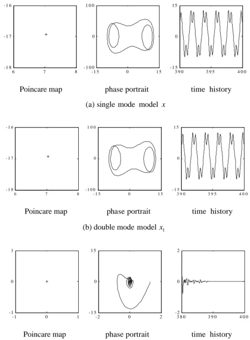
According to the nonlinear dynamic Eqs (16) and (17), the following numerical computations are carried out by the P-T method [10]. The parameters used are those as indicated in Eq. (18). The initial conditions of the numerical simulations for the single mode model arex= 0.0, andx˙ = 0.0ast= 0For the double mode model, the initial conditions arex1= 0.0,x˙1= 0.0,x2= 0.00001,x˙2= 0.0ast= 0
6 7 8 - 1 8
- 1 7 - 1 6
- 1 5 0 1 5
- 1 0 0 0 1 0 0
3 9 0 3 9 5 4 0 0
- 1 5 0 1 5
Poincare map phase portrait time history (a) single mode model x
6 7 8
- 1 8 - 1 7 - 1 6
- 1 5 0 1 5 - 1 0 0
0 1 0 0
3 9 0 3 9 5 4 0 0 - 1 5
0 1 5
Poincare map phase portrait time history (b) double mode model x 1
- 1 0 1
- 1 0 1
- 2 0 2
- 1 5 0 1 5
3 8 0 3 9 0 4 0 0
- 2 0 2
Poincare map phase portrait time history
(The vertical axis is amplified by 10 times) 65
(c) double mode model x2
Fig. 3. Comparison between single and double mode models (ω=π, g= 610).
The displacement modes used in this paper based on the single and double mode models can be expressed as follows.
w(x, y, t) =x(t) sinπx
L sin
πy
R, for the single mode model (47)
W∗(x, y, t) =x1(t) sinπx
L sin
πy
R +x2(t) sin
2πx
L sin
πy
5 1 0 1 5 - 1 0 0
0 1 0 0
- 2 0 0 2 0
- 2 0 0 0 2 0 0
3 8 0 3 9 0 4 0 0
- 2 0 0 2 0
Poincare map phase portrait time history (a) single mode model x
5 1 0 1 5
- 1 0 0 0 1 0 0
- 2 0 0 2 0
- 2 0 0 0 2 0 0
3 8 0 3 9 0 4 0 0
- 2 0 0 2 0
Poincare map phase portrait time history (b) double mode model x 1
- 1 0 1
- 1 0 1
- 1 0 1
- 1 0 0 1 0
3 8 0 3 9 0 4 0 0
-0.6 0 0.6
Poincare map phase portrait time history
(The vertical axis is amplified by 10 times) 21 (c) double mode modelx 2
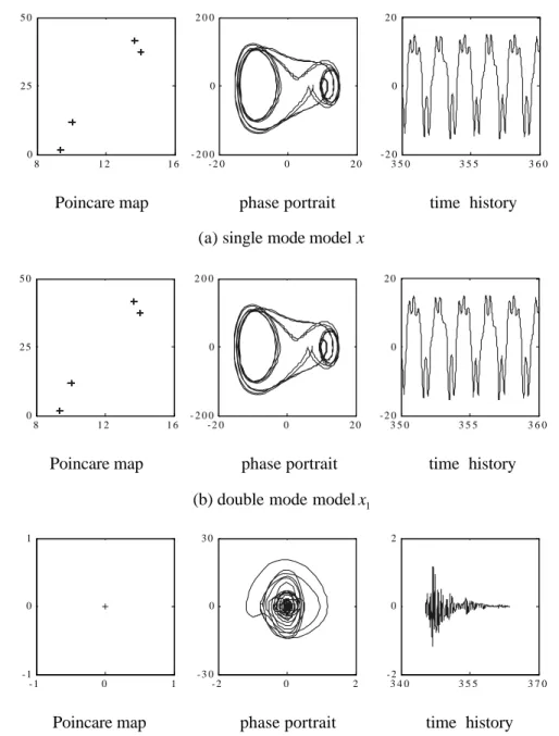
Fig. 4. Comparison between single and double mode models (ω=π, g= 1400).
If the single mode model is tenable, the following expression should be true.
W(x, y, t)≈W∗(x, y, t), x(t)≈x1(t), x2(t)−x1(t)
x1(t)
<<1 (49)
As can be seen from Fig. 3 to Fig. 5, the results obtained from the single and double mode models are completely identical when,ω =π,g = 610,ω =π,g = 1400andω =π,g = 1400if the other parameters are kept as the same. This is to say; in these cases the single mode model analysis is sufficient and correct.
8 1 2 1 6 0
2 5 5 0
- 2 0 0 2 0
- 2 0 0 0 2 0 0
3 5 0 3 5 5 3 6 0
- 2 0 0 2 0
Poincare map phase portrait time history (a) single mode model x
8 1 2 1 6
0 2 5 5 0
- 2 0 0 2 0
- 2 0 0 0 2 0 0
3 5 0 3 5 5 3 6 0
- 2 0 0 2 0
Poincare map phase portrait time history
(b) double mode modelx 1
- 1 0 1
- 1 0 1
- 2 0 2
- 3 0 0 3 0
3 4 0 3 5 5 3 7 0
- 2 0 2
Poincare map phase portrait time history
(The vertical axis is amplified by 10 times) 32
(c) double mode modelx 2
Fig. 5. Comparison between single and double mode models (ω= 1.1π,g= 1400).
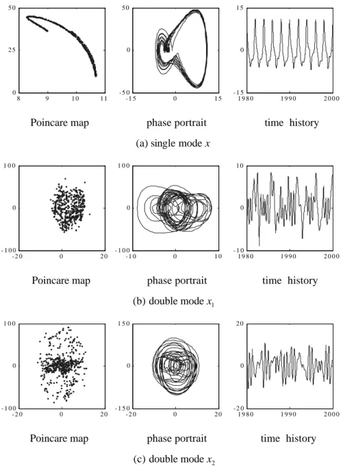
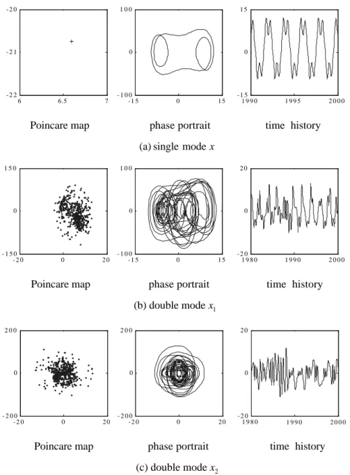
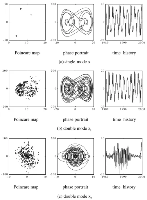
As illustrated in Fig. 6, 7 and 8, the single and double mode models generate completely different results. Chaotic behavior of the motion is identified by the results of the double mode model for the cases in which x2(tx1)−(tx1)(t)<<1
is not satisfied; whereas the corresponding results created by the single mode model indicate periodic or quasiperiodic behavior as shown in the figures. In other words, the single mode method, which is widely used in the dynamic analysis, may lead to incorrect conclusions in these cases. It is therefore clear that the single mode method has limits in analyzing the elastic structure’s nonlinear response. For the cases as indicated above, double mode or higher order mode method should be used for reliable results.
8 9 1 0 1 1 0
2 5 5 0
- 1 5 0 1 5
- 5 0 0 5 0
1 9 8 0 1 9 9 0 2 0 0 0
- 1 5 0 1 5
Poincare map phase portrait time history (a) single mode x
- 2 0 0 2 0
- 1 0 0 0 1 0 0
- 1 0 0 1 0
- 1 0 0 0 1 0 0
1 9 8 0 1 9 9 0 2 0 0 0
- 1 0 0 1 0
Poincare map phase portrait time history (b) double modex 1
- 2 0 0 2 0
- 1 0 0 0 1 0 0
- 2 0 0 2 0
- 1 5 0 0 1 5 0
1 9 8 0 1 9 9 0 2 0 0 0
- 2 0 0 2 0
Poincare map phase portrait time history (c) double modex 2
Fig. 6. Comparison between single and double mode models (ω=π, g= 200).
5. Concluding remarks
The characteristics of the nonlinear transverse vibration of an elastic cylindrical shell with large deflection and under uniform harmonic excitations are investigated in the present research based on the single and double mode models. In the current literature, systematical studies on such a shell exerted by multiple loadings are not found. Dynamic nonlinear modal equations for the motion of the cylindrical shell are derived on the basis of the models. Two types of nonlinear dynamic equations are obtained with a variety of system and loading parameters. Chaotic behavior of the cylindrical shell is evident as found in the present research. The criteria of chaos are determined for the motion of the cylindrical shell with the Melnikov function for the single mode model. Differences between the single and double mode models are apparent and a comparison between the results generated by the single and double mode models is carried out using numerical computations via the P-T method.
6 6.5 7 - 2 2
- 2 1 - 2 0
- 1 5 0 1 5
- 1 0 0 0 1 0 0
1 9 9 0 1 9 9 5 2 0 0 0
- 1 5 0 1 5
Poincare map phase portrait time history (a) single mode x
- 2 0 0 2 0
- 1 5 0 0 1 5 0
- 1 5 0 1 5
- 1 0 0 0 1 0 0
1 9 8 0 1 9 9 0 2 0 0 0
- 2 0 0 2 0
Poincare map phase portrait time history (b) double modex 1
- 2 0 0 2 0
- 2 0 0 0 2 0 0
- 2 0 0 2 0
- 2 0 0 0 2 0 0
1 9 8 0 - 2 0
0 2 0
Poincare map phase portrait time history (c) double modex2
1 9 9 0 2 0 0 0
Fig. 7. Comparison between single and double mode models (ω=π, g= 500).
Based on the theoretical and numerical analyses of the present research, it can also be stated thatW2(ξ, t) = T1(t)W1∗(ξ) +T2(t)W2∗(ξ)of the double mode model is close toW1(ξ, t) =T(t)W1∗(ξ)of the single mode model, provided thatx2(tx1)−(tx1)(t)<<1is complied. However,w2(ξ, t)is a better approximation solution overW1(ξ, t), when the conditions ofT1T((tt))≈1andT1(t)W2∗(ξ)−T1(t)W1∗(ξ)
T1(t)W∗
1(ξ)
<<1are satisfied. In this case, ifT(t)is chaotic,
T1(t)is also chaotic correspondingly, and vice versa. When the condition T2(t)W2∗(ξ)−T1(t)W1∗(ξ)
T1(t)W∗
1(ξ)
<< 1is not
maintained, the single mode method, which is conventionally used in the literature for analyzing the nonlinear behavior of an elastic system, may lead to incorrect conclusions and is therefore no longer reliable. The double mode or higher order mode models should then be employed in these cases.
0 1 0 2 0 - 5 0
0 5 0
- 2 0 0 2 0
- 2 0 0 0 2 0 0
1 9 8 0 1 9 9 0 2 0 0 0
- 2 0 0 2 0
Poincare map phase portrait time history (a) single mode x
0 1 0 2 0
- 2 0 0 0 2 0 0
- 2 0 0 2 0
- 2 0 0 0 2 0 0
1 9 8 0 1 9 9 0 2 0 0 0
- 2 0 0 2 0
Poincare map phase portrait time history (b) double modex 1
- 1 0 0 1 0
- 1 0 0 0 1 0 0
- 1 0 0 1 0
- 2 0 0 0 2 0 0
1 9 8 0 1 9 9 0 2 0 0 0
- 1 0 0 1 0
Poincare map phase portrait time history (c) double modex2
Fig. 8. Comparison between single and double mode models (ω=π, g= 1500).
Acknowledgement
This research is supported by NSERC, CFI and NNSFC.
References
[1] P. Holms and J. Marsden, A Partial Differential Equation with Infinitely Many Periodic Orbits: Chaotic Oscillation of a Forced Beam,
Arch. Rat. Mech. and Analysis 2 (1981), 135–165.
[2] F.C. Moon and S.W. Shaw, Chaotic Vibration of A Beam with Nonlinear Boundary Conditions, Non-linear Mech 18 (1983), 230–240. [3] P.D. Baran, Mathematical Models Used in Studying the Chaotic Vibration of Buckled Beam, Mechanics Research Communications 21
[4] V. Keragiozov and D. Keoagiozova, Chaotic Phenomena in the Dynamic Buckling of an Elastic-Plastic Column Under an Impact, Nonlinear
Dynamics 13 (1995), 1–16.
[5] G. Suire and G. Cederbaum, Periodic and Chaotic Behavior of Viscoelastic Nonlinear (Elastica) Bars under Harmonic Excitations 37 (1995), 753–772.
[6] S. Dwivedy and R. Kar, Dynamics of a Slender Beam with an Attached Mass under Combination Parametric and Internal Resonances, Part II: Periodic and Chaotic Responses, J. Sound Vib. 222 (1999), 281–305.
[7] X.L. Yang and P.R. Sethna, Nonlinear Forced Vibrations of a Nearly Square Plate-Antisymmetric Case, J. Sound Vib. 155 (1992), 413–441. [8] W. Tien, N. Namachchivaya and N. Malhotra, Non-Linear Dynamics of a Shallow Arch Under Periodic Excitation-II.1:1 Internal Resonance,
Int. J. Non-Linear Mech. 29 (1994), 367–385.
[9] Q. Han, H.Y. Hu and G.T. Yang, A Study of Chaotic Motion in Elastic Cylindrical Shells, Eur. J. Mech. A/Solids 18 (1999), 351–360. [10] L. Dai and M.C. Singh, A New Approach to Approximate and Numerical Solutions of Oscillatory Problems, J. Sound Vib. 263 (2003),
535–548.
[11] T. von Karman, Festigkeits Probleme in Machinenbau, Encl. Der math. Wiss. 4 (1910), 348–351. [12] A.C. Ugural, Stress in Plates and Shells, McGraw-Hill, Boston, 1999.
[13] S. Wiggins, Chaotic Transport in Dynamical Systems, Springer-Verlag, New York, 1992.
International Journal of
Aerospace
Engineering
Hindawi Publishing Corporationhttp://www.hindawi.com Volume 2010
Robotics
Journal ofHindawi Publishing Corporation
http://www.hindawi.com Volume 2014
Hindawi Publishing Corporation
http://www.hindawi.com Volume 2014
Active and Passive Electronic Components
Control Science and Engineering Journal of
Hindawi Publishing Corporation
http://www.hindawi.com Volume 2014
Rotating Machinery
Hindawi Publishing Corporation
http://www.hindawi.com Volume 2014
Hindawi Publishing Corporation http://www.hindawi.com
Journal of
Engineering
Volume 2014Submit your manuscripts at
http://www.hindawi.com
VLSI Design
Hindawi Publishing Corporation
http://www.hindawi.com Volume 2014
Hindawi Publishing Corporation
http://www.hindawi.com Volume 2014
Shock and Vibration
Hindawi Publishing Corporation
http://www.hindawi.com Volume 2014
Civil Engineering
Advances inAcoustics and VibrationAdvances in Hindawi Publishing Corporation
http://www.hindawi.com Volume 2014
Hindawi Publishing Corporation
http://www.hindawi.com Volume 2014 Electrical and Computer Engineering
Journal of
Advances in OptoElectronics
Hindawi Publishing Corporation
http://www.hindawi.com Volume 2014
The Scientific
World Journal
Hindawi Publishing Corporation
http://www.hindawi.com Volume 2014
Sensors
Journal of Hindawi Publishing Corporationhttp://www.hindawi.com Volume 2014
Modelling & Simulation in Engineering
Hindawi Publishing Corporation
http://www.hindawi.com Volume 2014
Hindawi Publishing Corporation
http://www.hindawi.com Volume 2014
Chemical Engineering
International Journal of Antennas and
Propagation
International Journal of
Hindawi Publishing Corporation
http://www.hindawi.com Volume 2014
Hindawi Publishing Corporation
http://www.hindawi.com Volume 2014
Navigation and Observation
International Journal of
Hindawi Publishing Corporation
http://www.hindawi.com Volume 2014