Privacy Preserving Data Publishing through Slicing

(1)

American Journal of Networks and Communications

2015; 4(3-1): 45-53

Published online February 10, 2015 (http://www.sciencepublishinggroup.com/j/ajnc) doi: 10.11648/j.ajnc.s.2015040301.18

ISSN: 2326-893X (Print); ISSN: 2326-8964 (Online)

Privacy preserving data publishing through slicing

Shivani Rohilla, Megha Sharma, A. Kulothungan, Manish Bhardwaj

Department of Computer science and Engineering, SRM University, NCR Campus, Modinagar, Ghaziabad, India

Email address:

[email protected] (S. Rohilla), [email protected] (M. Sharma), [email protected] (A. Kulothungan), [email protected] (M. Bhardwaj)

To cite this article:

Shivani Rohilla, Megha Sharma, A. Kulothungan, Manish Bhardwaj. Privacy Preserving Data Publishing through Slicing. American Journal of Networks and Communications. Special Issue: Ad Hoc Networks. Vol. 4, No. 3-1, 2015, pp. 45-53. doi: 10.11648/j.ajnc.s.2015040301.18

Abstract:

Microdata publishing should be privacy preserved as it may contain some sensitive information about an individual. Various anonymization techniques, generalization and bucketization, have been designed for privacy preserving microdata publishing. Generalization does not work better for high dimensional data. Bucketization failed to prevent membership disclosure and does not show a clear separation between quasi-identifiers and sensitive attributes. There are number of attributes in each record which can be categorized as 1) Identifiers such as Name or Social Security Number are the attributes that can be uniquely identify the individuals. 2)Some attributes may be Sensitive Attributes(SAs) such as disease and salary and 3) Some may be Quasi Identifiers (QI) such as zipcode, age, and sex whose values, when taken together, can potentially identify an individual. Data anonymization enables the transfer of information across a boundary, such as between two departments within an agency or between two agencies, while reducing the risk of unintended disclosure, and in certain environments in a manner that enables evaluation and analytics post-anonymization. Here, we present a novel technique called slicing which partitions the data both horizontally and vertically. It preserves better data utility than generalization and is more effective than bucketization in terms of sensitive attribute.

Keywords: PPDP, AG, CG, PT

1. Introduction

Data Anonymization is a technology that convert clear text into a non-human readable form. Data anonymization technique for privacy-preserving data publishing has received a lot of attention in recent years. Detailed data (also called as micro-data) contains information about a person, a household or an organization.

Data mining is the process of analysing data from different perspectives and summarizing it into useful information. Knowledge discovery from databases, techniques like clustering, association rules, regression, classification, decision trees, genetic algorithm etc. are used nowadays. Data mining is also used in areas of Science and Engineering such as genetics and bioinformatics.

In both generalization and bucketization, one first removes identifiers from the data and then partitions tuples into buckets. The two techniques differ in the next step. Generalization transforms the QI-values in each bucket into “less specific but semantically consistent” values so that tuples in the same bucket cannot be distinguished by their QI values. In bucketization, one separates the SAs from the QIs

by randomly permuting the SA values in each bucket. The anonymized data consists of a set of buckets with permuted sensitive attribute values.

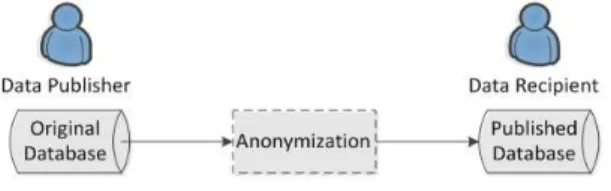
Fig. 1.1. Anonymization of data

(2)

46 Shivani Rohilla et al.: Privacy Preserving Data Publishing through Slicing

case for the examples of micro-data, e.g., census data and medical data. This thesis studies how we can publish and share micro data in a privacy-preserving manner. This present an extensive study of this problem along three dimensions: Designing a simple, intuitive, and robust privacy model, Designing an effective anonymization technique that works on sparse and high-dimensional data and developing a methodology for evaluating privacy and utility tradeoffs.

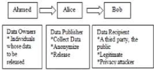
Fig. 1.2. Privacy preserving model for data

1.1. Organization

Here, we are studying slicing for privacy-preserving data publishing. Our contributions include the following. First, we introduce slicing as a new technique for privacy preserving data publishing. Slicing has several advantages when compared with generalization and bucketization. It preserves better data utility than generalization. It preserves more attribute correlations with the SAs than bucketization. It can also handle high-dimensional data and data without a clear separation of QIs and SAs.

Second, we show that slicing can be effectively used for preventing attribute disclosure, based on the privacy requirement of diversity. We introduce a notion called ℓ-diverse slicing, which ensures that the adversary cannot learn the sensitive value of any individual with a probability greater than 1/ℓ.

Third, we develop an efficient algorithm for computing the sliced table that satisfies ℓ-diversity. Our algorithm partitions attributes into columns, applies column generalization, and partitions tuples into buckets. Attributes that are highly-correlated are in the same column; this preserves the correlations between such attributes. The associations between uncorrelated attributes are broken; the provides better privacy as the associations between such attributes are less-frequent and potentially identifying.

Fourth, we describe the intuition behind membership disclosure and explain how slicing prevents membership disclosure. A bucket of size k can potentially match kc tuples where c is the number of columns. Because only k of the kc tuples are actually in the original data, the existence of the other kc −k tuples hides the membership information of tuples in the original data.

Finally, we conduct extensive workload experiments. Our results confirm that slicing preserves much better data utility than generalization. In workloads involving the sensitive attribute, slicing is also more effective than bucketization. In some classification experiments, slicing shows better

performance than using the original data (which may overfit the model). Our experiments also show the limitations of bucketization in membership disclosure protection and slicing remedies these limitations.

2. Existing Technology

There are two existing systems considered in this paper: Generalization and bucketization with which slicing is compared later.

Record linkage model attack and attribute linkage and attribute linkage model attack are different attacks occurred at the time of microdata publishing. There are some principles of privacy preserving as follows:-

2.1. K-Anonymity

Samarati and Sweeney introduced k-anonymity as the property that each record is indistinguishable with at least k-1 other records with respect to the quasi-identifier. In other words, k-anonymity requires that each QI group contains at least k records. k-anonymity is one of the most classic models, which prevents joining attacks by generalizing or suppressing portions of the released micro data so that no individual can be uniquely distinguished from a group of size k. k-Anonymity attributes are suppressed or generalized until each row is identical with at least k-1 other rows.

2.1.1. K-Anonymity using Generalization

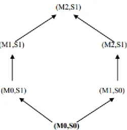
The generalization hierarchy transforms the k-anonymity problem into a partitioning problem. Specifically, this approach consists of the following two steps. The first step is to find a partitioning of the dimensional space, where n is the number of attributes in the quasi identifier, such that each partition contains at least k records. Then the records in each partition are generalized so that they all share the same quasi-identifier value. The Generalization method substitutes the values of a given attribute with more general values. Generalization can be applied at the following levels. Attribute Generalization (AG): generalization is performed at the level of column; a generalization step generalizes all the values in the column.

Cell Generalization (CG): generalization is performed on single cells; as a result a generalized table may contain, for a specific column, values at different generalization levels. There are two types of generalization exist namely domain generalization hierarchy and value generalization hierarchy. The domain generalization hierarchy of a domain topic is a lattice, where each vertex represents a generalized table that is obtained by generalizing the involved attributes according to the Corresponding domain tuple and by suppressing a certain number of tuples to fulfill the k-anonymity constraint.

(3)

American Journal of

Fig. 1.3. Domain generalization hierarchy

K-anonymity model for multiple sensitive mentioned that there are three kinds of information

1)Identity Disclosure: When an individual particular record in the published data disclosure.

2)Attribute Disclosure: When sensitive regarding individual is disclosed called as attribute

3)Membership Disclosure: When information individual’s information belongs from data not is disclosed is said to be membership disclosure.

2.1.2. Attacks on k-Anonymity

Here, we studied two attacks on

homogeneity attack and the background knowledge 1) Homogeneity Attack:

Sensitive information may be revealed based information if the non sensitive information is known to the attacker. If there is no sensitive attributes for a particular block getting sensitive information this method positive disclosure.

2) Background Knowledge Attack: If the user has some extra demographic can be linked to the released data which helps some of the sensitive attributes, then information about an individual might information. Such a method of revealing known as negative disclosure.

2.1.3. Limitations of k-Anonymity

(1) K-anonymity cannot hide whether a given in the database,

(2) K-anonymity reveals individuals' sensitive (3) K-anonymity cannot protect against background knowledge,

(4) Mere knowledge of the k-anonymization be violated by the privacy,

(5) K-anonymity does not applied to data without complete loss of utility.

(6) If a dataset is anonymized and pub

American Journal of Networks and Communications 2015; 4(3-1): 45-53

hierarchy

sensitive attributes information disclosure. individual is linked to a

called as identity

sensitive information attribute disclosure. information regarding

data set is present or disclosure.

k-anonymity: the knowledge attack.

based on the known information of an individual no diversity in the then it occurs. To is also known as

information which helps in neglecting then some sensitive might be revealing revealing information is

given individual is

sensitive attributes, against attacks based on

anonymization algorithm can

high-dimensional

published more than

once then special methods are required.

2.2. ℓ-Diverse Slicing

In the above example, tuple bucket. In general, a tuple t buckets. We now extend the above case and introduce the notion an adversary who knows all the infer t’s sensitive value from the to determine which buckets t matching buckets of t. Tuple matching buckets. Let p(t,B) bucket B (the procedure for described later in this section). example, p(t1,B1) = 1 and p(t1 the adversary computes p(t, s), sensitive value s. p(t, s) is calculated probability. Specifically, let p(s takes sensitive value s given

according to the law of total probability, is:

p(t, s) =∑b

In the rest of this section, we the two probabilities: p(t,B) and

Given a tuple t and a sliced bucket is in B depends on the fraction match the column values in B does not appear in the corresponding certain that t is not in B. In general, match |B|c tuples, where |B| is Without additional knowledge, column values are independent; tuples is equally likely to probability that t is in B depends tuples that match t.

We formalize the above analysis. between t’s column values {t[C column values {B[C1],B[C2], · ≤ c − 1) be the fraction of occurrences let fc(t,B) be the fraction of occurrences B[Cc − {S}]). Note that, Cc −

in the sensitive column. For example, = 1/4 = 0.25 and f2(t1,B1) = 2/ 0 and f2(t1,B2) = 0. Intuitively, degree on column Ci, between each possible candidate tuple original tuple, the matching degree product of the matching degree Q1_i_c fi(t,B). Note that Pt f( matching bucket of t, f(t,B) = matching buckets, t’s total matching is f(t) = PB f(t,B). The probability p(t,B) =f(t,B)/f(t)

Computing p(s|t,B). Suppose determine t’s sensitive value,

47

required.

tuple t1 has only one matching can have multiple matching above analysis to the general of ℓ-diverse slicing. Consider the QI values of t and attempts to the sliced table. He first needs may reside in, i.e., the set of Tuple t can be in any one of its is the probability that t is in for computing p(t,B) will be section). For example, in the above 1,B2) = 0. In the second step, ), the probability that t takes a calculated using the law of total s|t,B) be the probability that t that t is in bucket B, then probability, the probability p(t, s)

p(t,B)p(s|t,B) (1)

we will show how to compute and p(s|t,B).Computing p(t,B):

bucket B, the probability that t fraction of t’s column values that B. If some column value of t corresponding column of B, it is general, bucket B can potentially is the number of tuples in B. knowledge, one has to assume that the independent; therefore each of the |B|c be an original tuple. The depends on the fraction of the |B|c

analysis. We consider the match C1], t[C2], · · · , t[Cc]} and B’s · · · ,B[Cc]}. Let fi(t,B) (1 ≤ i occurrences of t[Ci] in B[Ci] and occurrences of t[Cc −{S}] in {S} is the set of QI attributes example, in Table 1(f), f1(t1,B1) /4 = 0.5. Similarly, f1(t1,B2) = Intuitively, fi(t,B) measures the matching tuple t and bucket B. Because tuple is equally likely to be an degree between t and B is the degree on each column, i.e.,f(t,B) = t,B) = 1 and when B is not a 0. Tuple t may have multiple matching degree in the whole data probability that t is in bucket B is:

(4)

48 Shivani Rohilla et al.:

sensitive column of bucket B. Since the contains the QI attributes, not all sensitive sensitive value. Only those sensitive values match t’s QI values are t’s candidate Without additional knowledge, all candidate (including duplicates) in a bucket are equally D(t,B) be the distribution of t’s candidate sensitive bucket B. Definition 6 (D(t,B)). Any sensitive associated with t[Cc − {S}] in B is a candidate value for t (there are fc(t,B) candidate sensitive B, including duplicates). Let D(t,B) be the candidate sensitive values in B and probability of the sensitive s in the distribution.

For example, in Table 1(f), D(t1,B1) = (dyspepsia 0.5) and therefore D(t1,B1)[dyspepsia] = 0

p(s|t,B) is exactly D(t,B)[s], i.e., p(s|t,B) =D Slicing. Once we have computed p(t,B) and able to compute the probability p(t, s) based (1). We can show when t is in the data, the takes a sensitive value sum up to 1.

Fact 1. For any tuple t ∈ D, Ps p(t, s) = 1. ℓ-Diverse slicing is defined based on the Definition(7) for ℓ-diverse slicing: A tuple diversity iff for any sensitive value s,

p(t, s) ≤ 1/ℓA sliced table satisfies ℓ-diversity tuple in it satisfies ℓ-diversity.

Our analysis directly show that from an table, an adversary cannot correctly learn the of any individual with a probability greater that once we have computed the probability a sensitive value, we can also use slicing measures such as t-closeness.

2.2.1. Attacks on L-Diversity

In this section we studied two attacks Skewness attack and the Similarity attack.

1) Skewness Attack :l-diversity cannot disclosure whenever the overall distribution satisfied.

2) Similarity Attack :When the sensitive are distinct but also semantically similar, learn important information.

2.2.2. Limitations of L-Diversity

While the l-diversity principle represents with respect to k-anonymity in protecting disclosure, it has several drawbacks. It is achieve l – Diversity and it also may not privacy protection.

3. Slicing

Generally in privacy preserving, there due to the presence of the adversary’s background in real life application. Data contains sensitive about individuals.These data when published privacy. The current practice in data publishing on policies and guidelines as to what types

Shivani Rohilla et al.: Privacy Preserving Data Publishing through Slicing

sensitive column sensitive values can be t’s values whose QI values sensitive values. candidate sensitive values equally possible. Let sensitive values in sensitive value that is candidate sensitive sensitive values for t in distribution of the D(t,B)[s] be the distribution.

dyspepsia :0.5, flu : .5. The probability D(t,B)[s].ℓ-Diverse and p(s|t,B), we are based on the Equation probabilities that t

1.

probability p(t, s). tuple t satisfies

ℓ-diversity iff every

an ℓ-diverse sliced the sensitive value greater than 1/ℓ. Note probability that a tuple takes slicing for other privacy

on l-diversity: the

cannot prevent attribute distribution is skewed and

sensitive attribute values an adversary can

represents an important step protecting against attribute is very difficult to provide sufficient

is loss of security background knowledge sensitive information published violate the publishing relies mainly types of data can be

published and on agreements The approach alone may lead to insufficient protection. Privacy (PPDP) provides methods and information while preserving data like bucketization, generalization privacy however they exhibit overcome this problem an algorithm

3.1. Architecture of Slicing and

Fig. 1.4. Slicing

Let T be the microdata table attributes: A = {A1,A2, . . . ,A are {D[A1],D[A2], . . . ,D[A represented as t = (t[A1], t[A2] ≤ d) is the Ai value of t.

Definition 1 (Attribute partition partition consists of several attribute belongs to exactly attributes is called a column. columns C1,C2, . . . ,Cc, then ∪ i1 6= i2 ≤ c, Ci1 ∩ Ci2 = ∅.

For simplicity of discussion, sensitive attribute S. If the data attributes, one can either consider consider their joint distribution.

contains S. Without loss of generality, contains S be the last column C the sensitive column. All other contain only QI attributes.

Definition 2 (Tuple partition consists of several subsets of T to exactly one subset. Each subset Specifically, let there be b buckets i=1Bi = T and for any 1 ≤ ∅.Definition 3 (Slicing). Given of T is given by an attribute partition For example, Table 1(e) and Table In Table 1(e), the attribute

Slicing

on the use of published data. to excessive data distortion or Privacy-preserving data publishing and tools for publishing useful data privacy. Many algorithms generalization have tried to preserve exhibit attribute disclosure. So to

algorithm called slicing is used.

and Formulization

Slicing Architecture

table to be published. T contains d ,Ad} and their attribute domains Ad]}. A tuple t ∈ T can be 2], ..., t[Ad]) where t[Ai] (1 ≤ i

partition and columns). An attribute subsets of A,such that each one subset. Each subset of column. Specifically, let there be c

∪c i=1Ci = A and for any 1 ≤

discussion, we consider only one data contains multiple sensitive consider them separately or distribution. Exactly one of the c columns generality, let the column that Cc. This column is also called other columns {C1,C2, . . . ,Cc−1}

and buckets). A tuple partition T, such that each tuple belongs subset of tuples is called a bucket. buckets B1,B2, . . . ,Bb, then ∪b

(5)

American Journal of Networks and Communications 2015; 4(3-1): 45-53 49

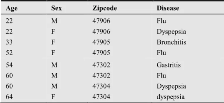
{Zipcode}, {Disease}} and the tuple partition is {{t1, t2, t3, t4}, {t5, t6, t7, t8}}. In Table 1(f), the attribute partition is {{Age, Sex}, {Zipcode, Disease}} and the tuple partition is {{t1, t2, t3, t4}, {t5, t6, t7, t8}}. Often times, slicing also involves column generalization.

Definition 4 (Column Generalization). Given a microdata table T and a column Ci = {Ai1,Ai2, . . . ,Aij}, a column generalization for Ci is defined as a set of non-overlapping j-dimensional regions that completely cover D[Ai1] × D[Ai2] × . . . × D[Aij ]. A column generalization maps each value of Ci to the region in which the value is contained.

Column generalization ensures that one column satisfies the k-anonymity requirement. It is a multidimensional encoding and can be used as an additional step in slicing. Specifically, a general slicing algorithm consists of the following three phases: attribute partition, column generalization, and tuple partition. Because each column contains much fewer attributes than the whole table, attribute partition enables slicing to handle high-dimensional data. A key notion of slicing is that of matching buckets.

Definition 5 (Matching Buckets). Let {C1,C2, . . . ,Cc} be the c columns of a sliced table. Let t be a tuple, and t[Ci] be the Ci value of t. Let B be a bucket in the sliced table, and B[Ci] be the multiset of Ci values in B. We say that B is a matching bucket of t iff for all 1 ≤ i ≤ c, t[Ci] ∈ B[Ci]. For example, consider the sliced table shown in Table 1(f), and consider t1 = (22,M, 47906, dyspepsia). Then, the set of matching buckets for t1 is {B1}.

Table 1: An original microdata table and its anonymized versions using various anonymization techniques

Table 1(a). The original table

Age Sex Zipcode Disease

22 M 47906 Dyspepsia

22 F 47906 Flu

33 F 47905 Flu

52 F 47905 Bronchitis

54 M 47302 Flu

64 F 47304 Gastritis

Table 1(b). The generalized table

[20-52] [20-52] [20-52] [20-52] * * * * 4790* 4790* 4790* 4790* Dyspepsia Flu Flu Bronchitis [54-64] [54-64] [54-64] [54-64] * * * * 4730* 4730* 4730* 4730* Flu Dyspepsia Dyspepsia Gastritis

Table 1(c). The Bucketized table

22 22 33 52 M F F F 47906 47906 47905 47905 Flu Dyspepsia Bronchitis Flu 54 60 60 64 M M M F 47302 47302 47304 47304 Gastritis Flu Dyspepsia dyspepsia

Table 1(d). Multiset based generalization

22:2,33:1, 52:1 22:2,33:1, 52:1 22:2,33:1, 52:1 22:2,33:1, 52:1 M:1,F:3 M:1,F:3 M:1,F:3 M:1,F:3 47905:2, 47906:2 47905:2, 47906:2 47905:2, 47906:2 47905:2, 47906:2 Dyspepsia Flu Flu Bronchitis 54:1,60:2, 64:1 54:1,60:2, 64:1 54:1,60:2, 64:1 54:1,60:2, 64:1 M:3,F:1 M:3,F:1 M:3,F:1 M:3,F:1 47302:2, 47304:2 47302:2, 47304:2 47302:2, 47304:2 47302:2, 47304:2 Flu Dyspepsia Dyspepsia Gastritis

Table 1(e). One attribute per column slicing

22 22 33 52 F M F F 47906 47905 47906 47905 Flu Flu Dyspepsia Bronchitis 54 60 60 64 M F M M 47302 47304 47302 47304 Dyspepsia Gastritis Dyspepsia Flu

Table 1(f). The sliced table

(Age,Sex) (Zipcode,Disease)

(22,M) (22,F) (33,F) (52,F) (47905,Flu) (47906,Dysp.) (47905,Bronchitis) (47906,Flu) (54,M) (60,M) (60,M) (64,F) (47304,Gast.) (47302,Flu) (47302,Dysp.) (47304,Dysp.)

3.2. Comparison with Generalization

(6)

recoding. In local recoding, one first groups tuples into buckets and then for each bucket, one replaces all values of one attribute with a generalized value. Such a recoding is local because the same attribute value may be generalized differently when they appear in different buckets. We now show that slicing preserves more information than such a local recoding approach, assuming that the same tuple partition is used. We achieve this by showing that slicing is better than the following enhancement of the local recoding approach. Rather than using a generalized value to replace more specific attribute values, one uses the multiset of exact values in each bucket. For example, Table 1(b) is a generalized table, and Table 1(d) is the result of using multisets of exact values rather than generalized values. For the Age attribute of the first bucket, we use the multiset of exact values {22,22,33,52} rather than the generalized interval. The multiset of exact values provides more information about the distribution of values in each attribute than the generalized interval. Therefore, using multisets of exact values preserves more information than generalization. However, we observe that this multiset-based generalization is equivalent to a trivial slicing scheme where each column contains exactly one attribute, because both approaches preserve the exact values in each attribute but break the association between them within one bucket. For example, Table 1(e) is equivalent to Table 1(d). Now comparing Table 1(e) with the sliced table shown in Table 1(f), we observe that while one-attribute-per-column slicing preserves attribute distributional information, it does not preserve attribute correlation, because each attribute is in its own column. In slicing, one groups correlated attributes together in one column and preserves their correlation. For example, in the sliced table shown in Table 1(f), correlations between Age and Sex and correlations between Zipcode and Disease are preserved. In fact, the sliced table encodes the same amount of information as the original data with regard to correlations between attributes in the same column. Another important advantage of slicing is its ability to handle high dimensional data. By partitioning attributes into columns, slicing reduces the dimensionality of the data.

Each column of the table can be viewed as a sub-table with a lower dimensionality. Slicing is also different from the approach of publishing multiple independent sub-tables in that these sub-tables are linked by the buckets in slicing.

3.3. Comparison with Bucketization

To compare slicing with bucketization, we first note that bucketization can be viewed as a special case of slicing, where there are exactly two columns: one column contains only the SA, and the other contains all the QIs. The advantages of slicing over bucketization can be understood as follows. First, by partitioning attributes into more than two columns, slicing can be used to prevent membership disclosure. Our empirical evaluation on a real dataset shows that bucketization does not prevent membership disclosure. Second, unlike bucketization, which requires a clear separation of QI attributes and the sensitive attribute, slicing

can be used without such a separation. For dataset such as the census data, one often cannot clearly separate QIs from SAs because there is no single external public database that one can use to determine which attributes the adversary already knows. Slicing can be useful for such data. Finally, by allowing a column to contain both some QI attributes and the sensitive attribute, attribute correlations between the sensitive attribute and the QI attributes are preserved. For example, in Table 1(f), Zipcode and Disease form one column, enabling inferences about their correlations. Attribute correlations are important utility in data publishing. For workloads that consider attributes in isolation, one can simply publish two tables, one containing all QI attributes and one containing the sensitive attribute.

3.4. Privacy Threats

When publishing microdata, there are three types of privacy disclosure threats. The first type is membership disclosure. When the dataset to be published is selected from a large population and the selection criteria are sensitive (e.g. only diabetes patients are selected), one needs to prevent adversaries from learning whether one’s record is included in the published dataset.

The second type is identity disclosure, which occurs when an individual is linked to a particular record in the released table. In some situations, one wants to protect against identity disclosure when the adversary is uncertain of membership. In this case, protection against membership disclosure helps protect against identity disclosure. In other situations, some adversary may already know that an individual’s record is in the published dataset, in which case, membership disclosure protection either does not apply or is insufficient.

The third type is attribute disclosure, which occurs when new information about some individuals is revealed, i.e., the released data makes it possible to infer the attributes of an individual more accurately than it would be possible before the release. Similar to the case of identity disclosure, we need to consider adversaries who already know the membership information. Identity disclosure leads to attribute disclosure. Once there is identity disclosure, an individual is re-identified and the corresponding sensitive value is revealed. Attribute disclosure can occur with or without identity disclosure, e.g., when the sensitive values of all matching tuples are the same.

For slicing, we consider protection against membership disclosure and attribute disclosure. It is a little unclear how identity disclosure should be defined for sliced data (or for data anonymized by bucketization), since each tuple resides within a bucket and within the bucket the association across different columns are hidden. In any case, because identity disclosure leads to attribute disclosure, protection against attribute disclosure is also sufficient protection against identity disclosure.

(7)

previous work on generalization and bucketization, where each tuple can belong to a unique equivalence-class (or bucket). In fact, it has been recognized that restricting a tuple in a unique bucket helps the adversary but does not improve data utility. We will see that allowing a tuple to match multiple buckets is important for both attribute disclosure protection and attribute disclosure protection.

4. Methodology

The key intuition that slicing provides privacy protection is that the slicing process ensures that for any tuple, there are generally multiple matching buckets. Slicing first partitions attributes into columns. Each column contains a subset of attributes. Slicing also partition tuples into buckets. Each bucket contains a subset of tuples. This horizontally partitions the table. Within each bucket, values in each column are randomly permutated to break the linking between different columns. This algorithm consists of three phases: attribute partitioning, column generalization, and tuple partitioning. We now describe the three phases:-

4.1. Attribute Partitioning

Highly correlated attributes are grouped together into one column in this attribute partitioning technique.There are three steps :

4.1.1. Equal Width Partitioning

There are two types of attribute: continuous and categorical. So, in this step, continuous attribute are converted into categorical attribute.

In equal width partitioning, we first divide the range into N intervals of equal size: uniform grid if A and B are the lowest and highest values of the attribute.

Width of intervals will be W=(B-A)/N

4.1.2. Measures of Correlation

Here,we calculate relation between two attributes..Let two attributes A₁ and A₂ with domains {V₁₁,V₁₂,……….V₁n₁} and {V₂₁,V₂₂,………V₂n₂} respectively. Their domain sizes are thus n₁ and n₂. Therefore, Mean square contingency coefficient formula is used.

4.1.3. Attribute Clustering

In this step,k-medoid clustering algorithm is used to partition attribute into columns as follows:-

The most common realisation of k-medoid clustering is the Partitioning Around Medoids (PAM) algorithm:

Algorithm 1.1

1. Initialize: randomly select (without replacement) k of the n data points as the medoids

2. Associate each data point to the closest medoid. ("closest" here is defined using any valid distance metric, most commonly Euclidean distance, Manhattan distance or Minkowski distance)

3. For each medoid m

For each non-medoid data point o

Swap m and o and compute the total cost of the

configuration

4. Select the configuration with the lowest cost.

5. Repeat steps 2 to 4 until there is no change in the medoid.

There can be a cluster based attribute slicing algorithm also as in existing systems, equal width discretization is used so it cannot handle skew data properly.So,to solve this problem,we proposed a new algorithm in proposed method,we use cluster based attribute algorithm for converting the continuous attribute into categorical attribute.This algorithm shows:

Input: Vector of real valued data a=(a₁,a₂…….a₁₁) and number of clusters to be determined k.

Goal: To find partition of data in k distinct clusters. Output: The set of cut points tₒ,t₁……...tk with tₒ<t₁<……..tn that defines discretization of adom(A).

Algorithm 1.2:

1. Compute amax=max{a₁,a₂,…….an} and

amin=min{a₁,a₂………..an}

2. Choose the centres as the first k distinct values of the attribute A.

3. Arrange them in increasing order

i.e.c[1]<c[2]<………c[k]. 4. Define boundary points bo=amin,

bj = (c[j]+c[j+1]) /2 for j=1 to k-1, bk=amax 5. Find the closest cluster to ai.

6. Recompute the centres of the cluster as the average of the values in each cluster.

7. Find the closest cluster to ai from the possible clusters {j-1,j,j+1}

8. Determination of cut points:- tₒ = amin

for i= 1to k-1 do

ti=(c[i]+c[i+1]) /2

9. end for

10. tk=amax

11. Apply formula of measures of correlation 12. Apply attribute clustering algorithm 13. Apply attribute partitioning algorithm

4.2. Column Generalization

First, column generalization may be required for identity/membership disclosure protection. If a column value is unique in a column, a tuple with this unique column value can only have one matching bucket. This is not good for

privacy protection as in the case of

generalization/bucketization where each tuple can belong to one equivalent class.

Given microdata table T and column

Ci={Ai1,Ai2,…..Aij}

Column generation for Ci is defined as set of non-overlapping j-dimensional regions that completely cover D[Ai1] x D[Ai2] x ……. D[Aij]

Column gen. maps each value of Ci to the region in which the value is contained.

(8)

protection and privacy protection.

4.3 Tuple Partitioning

The algorithm maintains two data structures: 1) A queue of buckets Q and

2) A set of sliced buckets SB.

Initially, Q contains only one bucket which includes all tuples and SB is empty. For each iteration, the algorithm removes a bucket from Q and splits the bucket into two buckets . If the sliced table after the split satisfies l-diversity, then the algorithm puts the two buckets at the end of the queue Q Otherwise, we cannot split the bucket anymore and the algorithm puts the bucket into SB.When Q becomes empty, we have computed the sliced table. The set of sliced buckets is SB.

Algorithm 1.3 for Tuple partitioning

1. Q = {T}, SB = ϕ. 2. While Q is not empty

3. Remove the first bucket B from Q, Q = Q − {B}. 4. Split B into two buckets B1 and B2, as in Mondrian. 5. If diversity-check (T, Q ∪ {B1, B2} ∪ SB, ℓ) 6. Q = Q ∪ {B1, B2}.

7. Else SB = SB ∪ {B}. 8. Return SB.

Algorithm 1.4 for Diversity-Check

1. For each tuple t ∈ T, L[t] = ϕ.

2. For each b 3. Record f (v) for each column value v in bucket B.

4. for each tuple t ∈ T

5. Calculate p(t,B) and find D(t,B). 6. L[t] = L[t] ∪ {hp (t, B), D (t, B) i}. 7. for each tuple t ∈ T

8. Calculate p(t, s) for each s based on L[t]. 9. If p(t, s) ≥ 1/ℓ, return false.

10. Return true…buckets B in T*

5. Experimental Results

5.1. Membership Disclosure Protection

We evaluate the effectiveness of slicing in membership disclosure protection. We first show that bucketization is vulnerable to membership disclosure. In both the OCC-7 dataset and the OCC-15 dataset, each combination of QI values occurs exactly once. This means that the adversary can determine the membership information of any individual by checking if the QI value appears in the bucketized data. If the QI value does not appear in the bucketized data, the individual is not in the original data. Otherwise, with high confidence, the individual is in the original data as no other individual has the same QI value.

We then show that slicing does prevent membership disclosure. We perform the following experiment. First, we partition attributes into c columns based on attribute correlations. We set c ∈ {2, 5}. In other words, we compare 2-column-slicing with 5-column-slicing. For example, when we set c = 5, we obtain 5 columns. In OCC-7,{Age, Marriage,

Gender} is one column and each other attribute is in its own column. In OCC-15, the 5 columns are: {Age, Work class, Education, Education-Num, Cap-Gain, Hours, Salary}, {Marriage, Occupation, Family, Gender}, {Race,Country}, {Final -Weight}, and {Cap-Loss}.

Then, we randomly partition tuples into buckets of size p (the last bucket may have fewer than p tuples). As described above, we collect statistics about the following two measures in our experiments: (1) the number of fake tuples and (2) the number of matching buckets for original v.s. the number of matching buckets for fake tuples. The number of fake tuples. Figure shows the experimental results on the number of fake tuples, with respect to the bucket size p. Our results show that the number of fake tuples is large enough to hide the original tuples. For example, for the OCC-7 dataset, even for a small bucket size of 100 and only 2 columns, slicing introduces as many as 87936 fake tuples, which is nearly twice the number of original tuples (45222). When we increase the bucket size, the number of fake tuples becomes larger. This is consistent with our analysis that a bucket of size k can potentially match kc –k fake tuples. In particular, when we increase the number of columns c, the number of fake tuples becomes exponentially larger. In almost all experiments, the number of fake tuples is larger than the number of original tuples. The existence of such a large number of fake tuples provides protection for membership information of the original tuples. The number of matching buckets. We categorize the tuples (both original tuples and fake tuples) into three categories: (1) ≤ 10: tuples that have at most 10 matching buckets, (2) 10−20: tuples that have more than 10 matching buckets but at most 20 matching buckets, and (3) > 20: tuples that have more than 20 matching buckets. For example, the “original-tuples(≤ 10)” bar gives the number of original tuples that have at most 10 matching buckets and the “fake-tuples(> 20)” bar gives the number of fake tuples that have more than 20 matching buckets. Because the number of fake tuples that have at most 10 matching buckets is very large, we omit the“fake-tuples(≤ 10)”bar from the figures to make the figures more readable.

(9)

grouping algorithms to ensure better protection against membership disclosure. The design of tuple grouping algorithms is left to future work.

6. Discussions and Future Work

A new approach called slicing is for privacy-preserving microdata publishing. Slicing overcomes the limitations of generalization and bucketization and preserves better utility while protecting against privacy threats. We illustrate how to use slicing to prevent attribute disclosure and membership disclosure. Our experiments show that slicing preserves better data utility than generalization and is more effective than bucketization in workloads involving the sensitive attribute.

The general methodology proposed by this work is that: before anonymizing the data, one can analyze the data characteristics and use these characteristics in data anonymization. The rationale is that one can design better data anonymization techniques when we know the data better.We show that attribute correlations can be used for privacy attacks.We have also shown that cluster based attribute slicing can also be done to achieve attribute partitioning.

This work motivates several directions for future research. First, in this paper, we consider slicing where each attribute is in exactly one column. An extension is the notion of

overlapping slicing, which duplicates an attribute in more than one columns. This releases more attribute correlations. For example, in Table 1(f), one could choose to include the Disease attribute also in the first column. That is, the two columns are {Age,Sex,Disease} and {Zipcode,Disease}. This could provide better data utility, but the privacy implications need to be carefully studied and understood. It is interesting to study the tradeoff between privacy and utility .

Second, we plan to study membership disclosure protection in more details. Our experiments show that random grouping is not very effective. We plan to design more effective tuple grouping algorithms.

Third, slicing is a promising technique for handling high-dimensional data. By partitioning attributes into columns,we protect privacy by breaking the association of uncorrelated attributes and preserve data utility by preserving the association between highly-correlated attributes. For example, slicing can be used for anonymizing transaction databases,

which has been studied recently in.

Finally, while a number of anonymization techniques have been designed, it remains an open problem on how to use the anonymized data. In our experiments, we randomly generate the associations between column values of a bucket.This may lose data utility. Another direction to design data mining tasks using the anonymized data computed by various anonymization techniques.

References

[1] Aggarwal.C, “On K-Anonymity and the Curse of Dimensionality,” Proc. Int‟l Conf.Very Large Data Bases (VLDB), 2005.

[2] Brickell.J and Shmatikov, “The Cost of Privacy:Destruction of Data Mining Utility in Anonymized Data Publishing”, Proc.ACM SIGKDD int‟l conf. Knowledge Discovery and Data Mining (KDD), 2008.

[3] Ghinita.G,Tao.Y, and Kalnis.P, “OnThe Anonymization of Sparse High Dimensional Data,” Proc. IEEE 24th Int‟l Conf. Data Eng. (ICDE), 2008.

[4] He.Y and Naughton.J, “Anonymization of Set-Valued Data via Top-Down, local Generalization,” Proc.IEEE 25th Int‟l Conf.Data Engineering (ICDE), 2009.

[5] Inan.A,Kantarcioglu.M,and Bertino.e, “Using Anonymized Data for Classification,” Proc. IEEE 25th Int‟l Conf. Data Eng. (ICDE), pp. 429-440, 2009.

[6] Li.T and Li.N, “On the Tradeoff between Privacy and Utility in Data Publishing,” Proc.ACM SIGKDD Int‟l Conf.Knowledge Discovery and Data Mining (KDD), 2009. [7] Li.N, Li.T, “Slicing: The new Approach for Privacy

Preserving Data publishing”, IEEE Transaction on knowledge and data Engineering, vol.24, No, 3, March 2012.

[8] L. Kaufman and P. Rousueeuw. Finding Groups in Data: an Introduction to Cluster Analysis. John Wiley& Sons, 1990. [9] X. Xiao and Y. Tao. Anatomy: simple and effective privacy

preservation. In VLDB, pages 139–150, 2006.

[10] X. Xiao and Y. Tao. Output perturbation with query relaxation. In VLDB, pages 857–869, 2008.