A Derivative-free Algorithm for
Finding Least Squares Solutions of
Quasi-linear and Linear Systems
Nikica Hlupi´c
1, Ivo Bero
s
ˇ
2and Danko Basch
31Department of Applied Computing, Faculty of Electrical Engineering and Computing, University of Zagreb, Croatia 2Department of Applied Mathematics and Computer Science, VERN’ University of Applied Sciences, Zagreb, Croatia 3Department of Control and Computer Engineering, Faculty of Electrical Engineering and Computing,
University of Zagreb, Croatia
A novel derivative-free algorithm for solving quasi-linear systems is presented. It resembles “classical” optimization approach but greatly simplifies computa-tion, resulting in fast execution and numerical stability. Though the global convergence cannot be guaranteed, it turns out that the presented algorithm finds a solution as successfully as other commonly accepted methods. The algorithm is clearly developed and mathematically founded, and its properties are examined by comparisons with other methods.
Keywords: derivative-free algorithm,optimization, quasi-linear systems, quasi-linear systems
1. Introduction
Quasi-linear systems are important because they are common in various fields of science, like mechanical and civil engineering or robotics and control theory, to mention a few of them. Although there are few theoretical results, like Bezout theorem[12], that provide some know-ledge about existence and number of solutions of such systems, there is no known analytical procedure to find them. Therefore, we try to compute solutions numerically and in practice we do not know in advance whether an exact solution exists at all, so we wish to find the best possible solution. Thus, we set the problem like the problem of minimization of residual sum of squares (rss) in the system and apply an opti-mization method to find solution according to least squares(LS). Because equations in quasi-linear system are easily differentiable, practi-cally all optimization methods can be tried and
the choice depends on the insight into the prob-lem and prior knowledge about possible solu-tions. So-calledline searchmethods like gradi-ent, Newton’s (Levenberg-Marquardt variant), Quasi-Newton and possibly conjugate gradient
[1],[13]will be good choice if we can find start-ing point not too distant from solution for other-wise they will likely find just a local optimum or not converge at all. If we do not have any clue about solution(i.e., we cannot even estimate it), the alternative is to apply derivative-free meth-ods like Nelder-Mead[1],[7],[13]. Finally, if the feasible set (possible values of unknowns) is closed(see, for example,[1])or if we have some prior knowledge about the feasible set, we can assign probabilities to candidate points. This opens the possibility for using various heuris-tics (simulated annealing, particle swarm, ant colony etc.; also called stochasticalgorithms)
and genetic algorithms, which can be effective as well[3],[7].
The main drawback of all these methods is that they search for better point only locally in some limited area around the current point
(limited either by the boundaries of feasible set or by knowledge about probability distribution of candidate points). In this paper we present an algorithm that overcomes this limitation[6]
benefit is a restricted set of search directions. This is quite a weak restriction because suit-able search directions are directions of coordi-nate axes, which are exactly the ones we would probably try as the first choice if we could freely choose direction. In the case that some other direction is unconditionally required, there is always the possibility to rotate the coordinate system so that one of coordinate axes becomes coincident with the desired direction. This is, in fact, what happens in so-called adaptive co-ordinate descent method [9]. Hence, arbitrary search directions are possible, but with a more involved computation. On the other hand, sim-plicity, numerical stability and success-fulness in solving systems of up to moderate complex-ity, indicated by simulations in the later sec-tions of the paper, confirm considerable practi-cal value of the proposed algorithm, even in its simplest form.
2. Mathematical Background and Formulation of the Algorithm
Quasi-linear systems are systems of nonlinear equations in which equations can consist not only of sums of unknowns multiplied by coeffi-cients, but also of mutual products of unknowns in all combinations. Formally, with vector of unknownsx= [x1x2. . .xn]T ∈Rn, quasi-linear
system is a system
F1(x)=f11(x)+f12(x)+. . .+f1q(x)=b1 F2(x)=f21(x)+f22(x)+. . .+f2q(x)=b2
...
Fm(x)=fm1(x)+fm2(x)+...+fmq(x)=bm
(1)
in which allf(x)are of the form[12]
f(x) =a·xp11x2p2. . .xpnn , (2) whereaare real numbers and powerspiare
ei-ther zero or one (pi = 0 means that variable
xi does not figure in f). Introducing notation
F:Rn →Rm,F(x) = [F1(x)F2(x). . .F m(x)]T
and b = [b1 b2. . .bm]T ∈ Rm, we write the
problem to be solved as
F(x) =b. (3)
The measure of the balance of each equation in the system is the difference ri = bi− Fi
be-tween its left and right sides, called residual. For convenience, we collect all residuals in a vector of residuals r = [r1 r2. . .rm]T ∈ Rm.
To solve the system means to find vectorxfor which all residuals will be zero. Since we do not know in advance whether such an xexists at all, the objective is to balance the system as well as possible, that is, to minimize residual sum of squares(rss)
rss=(bi−Fi)2=||r||2≥0, (4)
where the exact solution is found whenrss =0.
Minimization of rss is common optimization approach, but from here on, we continue in a different direction. While other methods try to determine all unknowns simultaneously, i.e., they search in all n dimensions, we compute only one variable at a time. This simplifies the problem by reducing its dimensionality at the cost of getting a better value of only one vari-able in the system, instead of all of them.
The idea of the algorithm is to update one by one variable and the key for this idea to be useful is a special computation which, as we shall see shortly, guarantees that updating any of the variables will improve the solution or, in the worst case, it will remain the same. The computation is based on considering all but one variable known and fixed in each step of the algorithm. Because the variable considered un-known changes, let us denote it by. To explain the computation, letx1, for example, be
consid-ered the only unknown and x2, . . . ,xn known
and fixed at their current values. Substituting known values into the system(1) and writting
instead ofx1we get a system of the form
a11· +a12· +. . .+a1q· =b1 a21· +a22· +. . .+a2q· =b2
...
am1· +am2· +. . .+amq· =bm.
(5)
Coefficients aij in (5)contain contributions of
all known variablesx2, . . . ,xnas well as of
(5)is nothing but
(a11+a12+...+a1q)·=v1·=b1 (a21+a22+...+a2q)·=v2·=b2
...
(am1+am2+...+amq)·=vm·=bm
(6)
or, withv= [v1v2. . .vn]T∈Rn, simply
v· =b. (7)
System(6), i.e.,(7)is a linear system ofm equa-tions in one unknown and its LS solution can be relatively simply computed as[5],[10],[14]
LS = (vTv)−1vTb=
m
i=1 vibi
m
i=1v 2
i
=
m
i=1 vibi
|v|2 . (8)
Formula (8) yields the best possible value (in the whole setR)of the variable considered un-known, with other variables fixed at their current values. The new value of the selected variable will certainly be better than the previous one because by Gauss-Markov theorem[5],[10],[14]
it is guaranteed that new rss will necessarily be less or, in the worst case, equal to the one obtained by the old value of the selected vari-able. The explained procedure is an efficient computational engine for minimizing rss in a single dimension that we shall use in higher-level algorithms, so let us call it quasi-linear computational engine(QLCE)and summarize here for convenience.
Algorithm 1: QLCE
1. Given the current point x and one of coor-dinate axes as search direction (let it be jth
axis), consider the corresponding variablexj
unknown.
2. In system(1)substitute current values for all variables considered known and denotexjas
. This will render the system into a linear system in of the form(6), i.e.,(7).
3. If||v|| =0, solve(7)for according to(8). Let us denote the result asLS. If||v|| =0,
just return some indication of failure to the calling routine.
4. Compose new point xnew by replacing xjin
xbyLS. Thisxnewminimizes therssof the
original system (1) in selected dimension
(i.e., along the line of selected coordinate axis).
Having QLCE computation at disposal, we im-mediately arrive to a natural extension of its underlying idea. The approach is to consider one by one variable unknown, with all other variables fixed at their current values, and to update them sequentially in order to gradually approach the solution, i.e.,rssminimizer. Such an algorithm certainly exhibits descent property
[1] because rss is necessarily reduced in each step (in the worst case it remains the same). Let us name it quasy-linear solver(QLS) and formulate it precisely.
Algorithm 2: quasi-linear solver(QLS) 1. Setx=starting pointx0.
2. forj=1 ton
• Considerxjunknown and apply QLCE to
find its better value. In the case of QLCE failure just return to the incremental part of the loop, i.e., take another variable as unknown and repeat QLCE computation.
• Here QLCE returned xnew. To use it in
further computation, setx=xnew.
3. Check stopping conditions and if none is sat-isfied, continue from the step 2.
Remark: in step 2b, it is sufficient to take only
jth component of x
new, that is, QLCE can be
stopped as soon asLSis obtained and only this
LShas to be substituted forxjto construct new
xin step 2b of QLS.
sequential updating of unknowns in some fixed order, we apply greedy[2]strategy. This means that in each iteration we check all dimensions
(every variable is once taken as the unknown and resulting rss is computed), but eventually we update only the variable for which achiev-able rssreduction is maximal. This is the un-derlying logic of the algorithm we call greedy quasi-linear solver(QLSG).
Algorithm 3: greedy quasi-linear solver(QLSG)
1. Given the current pointx, compute referen-tialrss, that is, setrssref =rss(x). Also, set rssmin =rssrefandxbest=x.
2. forj=1 ton
• Considerxj unknown and apply QLCE to
find its better value. In the case of QLCE failure just return to the incremental part of the loop, i.e., take another variable as unknown and repeat QLCE computation.
• Here QLCE returnedxnewso
computerssnew =rss(xnew).
• Ifrssnew<rssmin
setrssmin =rssnew andxbest=xnew.
3. Setx=xbest.
4. Check stopping conditions and if none is sat-isfied, continue from the beginning.
Remark: in steps 2a and 2b again we only need to work withLS, rather than with the wholex.
There are several possible stopping conditions and we discuss those that we use in the section on comparative study. Most of them are com-mon to the majority of optimization methods, but QLSG algorithm, specifically, has to care about ||v|| and prevent potential problem that
||v|| = 0 in(8), which is the task of step 3 in QLCE. In the early stages of QLSG this is a very unlikely situation because zero norm ofv(with nonzero b) means that the problem is not well defined and this, in turn, means that in the se-lected dimension improvement is not possible at all. However, as we approach the solution or a stationary point, numerical limitations can cause inability to solve (8) in any dimension, which is then indication for stopping the exe-cution. In fact, in that case x will not change at all so this can be detected by watching x, as is done routinely in other methods as well. In practice, such situations are relatively rare and
in the next section we present comparative study that confirms the merit of QLSG.
3. Comparative Study
We shall compare QLSG with two commonly accepted methods. Specifically, with New-ton’s method(Levenberg-Marquardt modifica-tion) that uses simple backtracking for line-searchand with Nelder-Mead method as a rep-resentative of derivative-free methods. Because solving quasi-linear systems is challenging only for systems with three or more equations and unknowns, visualization of algorithms advance is not feasible. Therefore, the main criterion for comparison will be successfulness of the al-gorithms in finding a solution, i.e., the quantity of interest in our work is the number of solved systems out of systems tried, that is, proportion of solved systems which we denote by. Reliable establishment of differences among the algorithms(i.e., proportions of solved sys-tems)requires some kind of analysis of variance
(ANOVA) [4],[11],[14], but to facilitate analy-sis of results, we construct confidence intervals for estimates of proportions and present them graphically. In experiments like ours, where we work with so-called count data[11], proportion is a variable having the binomial distribution. However, for large number of samples (more than 30, and we always have many more than that) we can use the normal approximation to the binomial distribution so we may compute confidence intervals according to[11]
ˆ
−z/2
ˆ
(1−ˆ)
n <<ˆ+z/2
ˆ
(1−ˆ) n ,
(9) where ˆ is the observed proportion of successes in n trials (n systems) and z/2 is the value of a standard normal variable corresponding to the degree (level)of confidence (1−). We use = 0,05, which means that there is 95% probability that true proportion lies within the confidence interval.
In all simulations we randomly generate quasi-linear systems with at least one known solution
the known solution are random integers in the range[−10,10]. Nelder-Mead simplex method is identical to Matlab variant implemented in fminsearch function, while QLSG and New-ton’s method (Levenberg-Marquardt) are the authors’ custom routines. Stopping conditions are the same for both:
1. sufficiently small gradient components
(smaller than 10−6)
2. insufficient change of solution compo-nents
(relative change smaller than 10−15)
3. insufficient reduction ofrss(relative reduc-tion smaller than 10−14)
4. maximal number of iterations exceeded. Starting point in all simulations is always the origin of coordinate system (zero-vector) and the system is considered solved if the final rss
drops below 10−6. This is an absolute
thresh-old, though “the optimal” threshold might be expected to be related to initialrssand the struc-ture of the system. However, absolute tresholds are justified and common in optimization be-cause in the case that we find “the right search path”, the algorithm can reduce rssarbitrarily, down to numerical precision of computer, so we can freely use any absolute threshold. On the other hand, if we take wrong direction, rss re-duction will be minor and even after thousands of iterations it would remain far above any rea-sonable threshold anyway. In such sitations it is much better to restart the algorithm(from some other starting point).
First we consider small systems of three equa-tions in three unknowns. We use notation e3x3q4, which means “equations 3”, “xes 3” and maximally 4 combinatorial terms (with products of unknowns) in an equation. Max-imal number of iterations is 20000 and we gen-erate 500 systems. Result of comparison is in Figure 1. We see that with these small systems QLSG is as successful as “classical” Levenberg-Marquardt(LM)algorithm, while both are bet-ter than Nelder-Mead method. Successfulness of QLSG and LM algorithm is about 75%, but insight into simulation output reveals that LM algorithm on average needs just 40 and QLSG about 3600 iterations. If we take into account the fact that LM in each iteration updates all unknowns and QLSG updates only one, fair
comparison requires that we divide total num-ber of QLSG iterations by the numnum-ber of vari-ables. With this correction, the average num-ber of QLSG iterations is 1200, which is still much more than LM needs. This is a typical outcome because LM search direction follows from the second-order Taylor approximation of the objective function, which is quite a good ap-proximation, while QLSG search directions are merely directions of coordinate axes so QLSG cannot take “shortcuts” on its way to the solu-tion. On the other hand, QLSG does not need derivatives and, more important, it does not re-quire equal number of equations and unknowns in the system, which is its second major advan-tage over Newton’s and similar methods.
Figure 1. Proportions of successes with systems e3x3q4 and 95% confidence intervals of proportions.
In real life applications, we usually encounter overdetermined systems[5],[10] (systems with more equations than unknowns)and they rarely have exact solution. Nevertheless, it is usually desirable to obtain the best possible, i.e., least squares, solution, even when we know that an exact one does not exist. QLSG(or QLS)is very usefully in such situations because it is designed to reducerssas much as possible and in that way, in effect, it tries to find least squares solution. There is, of course, no guarantee that QLSG will yield true least squares solution because it can finish in a local optimum or fail for some other reason. Also, there is no known closed form formula or algorithm that is guaranteed to yield least squares solution of a quasi-linear system, so it is not possible to verify QLSG re-sult anyway. Nonetheless, the fact is that QLSG reducesrssand thereby it approaches true least squares solution, whatever it be.
Fig-ure 2 and FigFig-ure 3 that show results for 500 systems e5x5q4 and e10x10q4, respectively.
Figure 2. Proportions of successes with systems e5x5q4 and 95% confidence intervals of proportions.
Figure 3. Proportions of successes with systems e10x10q4 and 95% confidence intervals of proportions.
We see that proportion of success(values on ab-scissa)rapidly decreases as complexity of sys-tem increases. Observing these figures, it could be concluded that QLSG continually becomes worse than LM as complexity of systems in-creases. This would, however, be a hasty con-clusion because the simulations allowed lim-ited number of iterations, which caused QLSG to end before it exhausted all its capabilities. When QLSG is let running until some other stopping condition (not number of iterations)
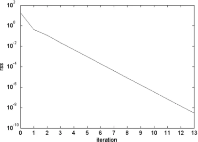
breaks the execution, it becomes as success-ful as LM, if not better. Unfortunately, in bad circumstances it can easily reach a few tens of thousands iterations before it finds solution, but it mostly does find it. This is illustrated in Figure 4, which shows QLSG performance for one of the systems e5x5q4 which has not been solved in previous simulation due to lim-ited number of iterations. The limit was 25000 iterations and, as before, the end point(the last
xvector)was considered a solution if the final
rss was less than 10−6. As we see in the fig-ure, for the system under consideration thisrss
value is reached at 26330thiteration and though QLSG can solve it, in the previous simulation it was counted as unsolved.
Figure 4. Log-log graph of typical course of solving e5x5q4 system, i.e.,rssreduction by QLSG algorithm.
The “trajectory” ofrssin Figure 4 shows a typi-cal course of advance of QLSG. In the beginning it quickly reducesrssfor few orders of magni-tude, but then it usually needs many iterations to make many small movements until it comes into “the basin of attraction” of a solution. Eventu-ally, once it gets close enough to the solution, the algorithm rapidly descends to it. Thus, if it is important to solve the system and time is not a limiting factor, QLSG might be the best algo-rithm for this task. This follows from the fact that QLCE computation yields the best point on the whole line of search direction, while other methods can search only locally in some limited area around the current point. Due to this prop-erty, QLSG has good chances to get out of local optimums and purely accidentally find solution, even when this is apparently not likely.
4. QLS Applied to Linear Systems
on comparative study remain in effect when it is applied to linear systems as well. However, ap-plying the basic(non-greedy)variant, i.e. QLS algorithm, to a linear system reveals a surprising connection between QLS algorithm and Gauss-Seidel method[5],[8]for solving linear systems. Namely, it turns out that, when applied to a pure linear systemAx =b, the QLS algorithm is nothing but another form of Gauss-Seidel method applied to the system ATAx = ATb. Thus, we can establish the following result.
Proposition: When applied to a linear sys-tem Ax = b, QLS algorithm is equivalent to Gauss-Seidel method applied to the system ATAx=ATb.
Proof: We prove the statement by showing that QLCE computation of new value of a single unknown, when applied to a linear system and sequentially to all unknowns, is algebraically equivalent to Gauss-Seidel computation. In each iteration, QLS algorithm applied to
Ax = btries to reduce rss(x) = r(x)Tr(x) =
||b−Ax||2 by changing only one x
k. To this
aim, it fixes all other unknowns and solves
d/dxk[rss(xk)] = 0. Expanded, the condition
d/dxk[rss(xk)] =0 is
2(b−x1·a1−. . .−xk·ak−. . .−xn·an)T·ak =0,
where aj means jth column of matrix A. By
isolatingxkit follows that newxkby QLS is
xk = (b−x1a1−. . .−xk−1ak−1
(ak)Tak
+ −xk+1ak+1(−a . . .−xnan)Tak
k)Tak .
(10)
If we introduce notation C = ATA and d = ATb and have in mind that matrix C is
symmetric, formula(10)can be written as
xk = dk−x1ck1−. . .c −xk−1ck,k−1 kk
+ −xk+1ck,k+1c−. . .−xnckn
kk .
(11)
On the other hand, new value of yk yielded by
Gauss-Seidel method, when applied to the sys-temCy=d, is given by
k−1
i=1
yicki+ykckk+ n
i=k+1
yicki=dk (12)
wherefrom we get
yk = cdk kk −
k−1
i=1
yicki− n
i=k+1 yicki
= dk−y1ck1−c. . .−yk−1ck,k−1
kk
+ −yk+1ck,k+1c−. . .−ynckn
kk .
(13)
Comparing new xk by QLS in (11) with new
yk by Gauss-Seidel method in (13), we see
that they are identical, so for any starting point
x(0) = y(0) the sequence of new values of un-knowns produced by either method will be iden-tical.
The equivalence of QLS and Gauss-Seidel me-thod sheds a new light on Gauss-Seidel meme-thod, but more importantly, it enables transferring of all theoretical results developed for Gauss-Seidel to QLS. Hence, because the conver-gence of Gauss-Seidel method, when applied to positive definite systems [5],[10], is proven
[5],[8], and ATA certainly is positive definite
[5],[8],[10], we may assert that convergence of QLS algorithm applied to any linear system is guaranteed as well. In the case that system has no solution at all, QLS algorithm will converge to a least squares solution x = (ATA)−1ATb,
which is a desired property.
Guaranteed convergence motivates further opti-mization of the algorithm with respect to specifics of linear systems in order to accelerate the algo-rithm as much as possible. Indeed, it is possible to reduce the number of operations by taking a deeper insight into a two consecutive steps, so let us follow what QLS does with system
Ax=b, which we expand here for convenience. We havemequations innunknowns
a11x1+a12x2+. . .+a1nxn=b1 a21x1+a22x2+. . .+a2nxn=b2
...
am1x1+am2x2+. . .+amnxn=bm.
(14)
QLS takes one unknown, let us sayx1, and
that do not containx1from the right sides in all
equations. Hence, QLS constructs the system
a11x1=b1−a12x2−. . .−a1nxn
a21x1=b2−a22x2−. . .−a2nxn
...
am1x1=bm−am2x2−. . .−amnxn
(15)
or in common matrix-vector notation
a1x1 =b−
n
j=2
ajxj. (16)
New x1 is obtained by solving (16) according
to (8), where a1from(16) has the role ofvin (7) and the right side of(16)has the role of b
in(7). In the next step QLS takesx2as the only
unknown and constructs
a2x2 =b−
n
j=1 j=2
ajxj, (17)
where it uses new x1 obtained in the previous
step. Looking at(16)and (17), we notice that by switching fromx1tox2, the right sides of the
systems to be solved contain mainly the same terms. The difference is only that in (16) we subtract a2x2, while in(17)this term does not
contribute to the right side and in(17)we sub-stracta1x1(newx1), which was not subtracted
in(16). Hence, once we compute the right side in (16), computing the right side in (17)does not require all calculations as given by the for-mula. It is sufficient to adda2x2to the right side
obtained by(16)in order to cancel subtraction ofa2x2in the previous step, and to subtracta1x1 (with newx1)from the result. If we denote the right sides of these systems when computing
xi asti, we can write all calculations needed to
transform the right side in two consecutive steps as a recursive formula
ti =ti−1+aixi−ai−1xi−1. (18)
Relation (18), along with the fact that the left sides of systems of the form(16)and(17)are simplyithcolumns of system matrixA, enables significant reduction of the number of needed operations and leads to a highly optimized vari-ant of the algorithm designed specifically for solving linear systems. Of course, because(18) is a recursive formula, the algorithm has to be
started properly as specified in the following list.
Algorithm 4: optimized linear solver 1. Setx=starting pointx0.
2. Compute all possible denominators in (8) that can appear(there will benof them)and store them appropriately, let us say in array den.
3. Compute the right side of(16)takingxn as
the unknown, that is, compute
tn =b− n−1
j=1 ajxj.
4. fori=1 ton
• Use recursive formula(18)to compute the right side of (16) for xi as the unknown,
that is, compute
ti =ti−1+aixi−ai−1xi−1.
If i = 1, use n instead of i−1 to prop-erly handle the circularity of sequence of variables.
• Solve aixi = ti for xi according to (8),
whereas the value of denominator is den[i]. Denote newxiasLS.
• Replacexiin the currentxbyLS.
5. Check stopping conditions and, if none is satisfied, start new sequence of updates, i.e., continue from step 4.
Step 2 is not necessary, but it accelerates cal-culation (8) in step 4b at the negligible cost of some extra storage. Step 3 is the required initialization of recursion as it simulates the non-existing previous state of recursion (state as would be before repeated arrival tox1). To illustrate the practical value of QLS and its properties when applied to a linear system, let us consider a simple example. System
x1+x2+x3=3 x1−x2+x3=3 x1−x2−x3=1
(19)
be easily found. In contrast, QLS(all variants)
does not have any problem with this system and the course of the algorithm’s advance(i.e., re-duction ofrss)is shown in Figure 5.
Figure 5. The course ofrssreduction when solving system(19)by QLS algorithm.
The equivalence of QLS and Gauss-Seidel me-thod applied to normalized system has been pro-ven algebraically and illustration, either graph-ical or tabular, cannot show anything but the same curves or numbers because both algo-rithms yield identical estimates of unknowns up to the numerical precision of the computer. Un-fortunately, precise calculation in the next sec-tion reveals that even optimized QLS algorithm requires about three times more basic operations
(additions, multiplications) than Gauss-Seidel method to solve system Ax = b, so there is not much reason to use it in practice. It is true that QLS can be directly applied to any sys-tem, while Gauss-Seidel method imposes cer-tain constraints, but if we wish LS solution of a system, there are other methods (like QR or SVD, see [5],[10])at disposal and they will likely be faster than QLS when applied to full systems. With sparse systems QLS algorithm might be competitive, but this strongly depends on implementation and is subject to additional examination out of the scope of this paper.
5. Complexity Analysis
Because all presented algorithms are iterative routines for which required number of iterations is not known in advance, the appropriate mea-sure of complexity is the number of operations in a single iteration.
Obviously, the complexity of the basic QLS variant (Algorithm 2) is n times the complex-ity of its computational engine QLCE and the number of operations in QLCE depends on the structure of equations and their terms. We know the largest numberqof terms in a single equa-tion in the system, but to facilitate the analysis and get the worse possible situation, we assume that all equations haveqterms and that all terms contain all unknowns. Then, when we fix all ex-cept one variable and substitute their values in a term like(2), calculation of the resulting co-efficient ars in (5) takes exactly (n −1) −1
multiplications (M) for multiplying variables plus one multiplication with coefficient, which yields the total ofn−1 multiplications. Process-ing allqterms in an equation requiresq(n−1)
multiplications and collecting the resulting co-efficients according to(6)requiresq−1 addi-tions(A). Hence, processing a single equation is
q(n−1)M+(q−1)A operation and processing the whole system to complete step 2 of QLCE requiresm[q(n−1)M+ (q−1)A]basic opera-tions. Solving(8)in the third step of QLCE will take additionalmmultiplications andm−1 addi-tions in both nominator and denominator, and fi-nally one division, which we shall(for simplic-ity)account for as multiplication. Thus, solving
(8)requires totally 2[mM+(m−1)A]+M basic operations. All in all, one QLCE iteration takes
[mq(n−1) +2(m+1)]multiplications and
[m(q−1) +2(m−1)]additions. (20)
In “big Oh” notation[2] this becomes O(mqn)
multiplications and O(mq) additions, so it fol-lows that QLCE has linear complexity with re-spect to all relevant parameters. Consequently, one iteration of QLS is
O(n[O(mqn)M+O(mq)A])
=O(mqn2)M+O(mqn)A. (21)
Form=nandqn, this becomes
O(n3)M+O(n2)A. (22)
Thus, it can be declared that in common situa-tions QLS is roughly O(n3)algorithm.
magnitude smaller number of operations. This is easy to obtain by the analysis analogous to the preceding one. The only difference is that
q = n and there will be only one multiplica-tion per term during construcmultiplica-tion of system(5). However, with linear systems we should use the optimized linear solver. Though its big Oh com-plexity is of the same order as that of general QLS when applied to linear systems, the asymp-totic complexity is smaller and can be important for large size problems. Let us now calculate it precisely.
Algorithm 4 has preprocessing phase (steps 2 and 3) and iterative phase (steps 4 and 5). In step 2 all denominators in (8) are computed and we have already found that this will take
mM+ (m−1)A per variable, that is, step 2 is
n[mM+ (m−1)A]. Initialization of recursion in step 3 requires(n−1)nM forn−1 products
ajxj, then [(n−1)−1]A for their summation
and finallynA for subtraction of the sum from
b or totally (n−1)nM+2(n−1)A. On the whole, the preprocessing phase requires
n[mM+(m−1)A]+(n−1)nM+2(n−1)A
=(nm+n2−n)M+[(m−1)+2(n−1)]A. (23)
Complexity of iterative phase depends on steps 4a and 4b. Clearly, recursion (18) in step 4a is 2nM +2nA. In step 4b we only have to compute nominator, which takes mM and
(m − 1)A. Denominator is looked-up from the storage prepared in advance, so step 4b is completed by just one additional division ( ac-counted for as multiplication). Thus, step 4b is (m +1)M+ (m−1)A and it follows that the total complexity of one pass through the for loop is 2nM+2nA+ (m+1)M+ (m−1)A or
(2n+m+1)M+ (2n+m−1)A. Updating all
nvariables is, consequently,
(2n2+nm+n)M+ (2n2+nm−n)A. (24) According to (23) and (24), the complexity of preprocessing and iterative phase is simi-lar, determined by terms (nm+n2−n)M and
(2n2+nm+n)M, respectively, but iterative term
is a little larger. Of course, the more iterations, the more important iterative term so in practice it will be dominant. Therefore, in a common situation, whenm=n, the complexity of linear solver is roughly 3n2 and it can be declared to be O(n2)algorithm.
For comparison, the update of a single variable by Gauss-Seidel method, according to (13), is precisely(n−1)M+[(n−1)−1]A+M+2A= nM+nA, so the update of allnvariables, i.e., one iteration, isn2M+n2A. Because
multipli-cation is much more time consuming than addi-tion, we can neglect addition term and it follows that complexity of Gauss-Seidel method isn2or about three times less than of the optimized lin-ear solver.
6. Conclusion
Quasi-linear solver presented in the paper is computationally one of the simplest algorithms for solving systems of quasi-linear equations ap-plying optimization approach but, at the same time, it shows to be one of the most robust and effective ones as well. Conceptually, the idea of the presented algorithm resembles coordinate descent method [9], but determining only one variable at a time is all that is common to these two algorithms. The main difference follows from the fact that QLS benefits from the spe-cial form of equations, which eventually leads to completely different computation. Compar-isons show that it is as successful as Levenberg-Marquardt variant of Newton’s method and they are both more successful than Nelder-Mead al-gorithm, when dealing with quasi-linear sys-tems. However, QLSG has three major advan-tages over Newton’s method when we deal with quasi-linear systems.
implementation and, together with simple and well defined computation of LS solution, re-duces numerical requirements.
All these advantages have been gained at a rel-atively low cost that search directions are re-stricted to directions of coordinate axes and that we update only one dimension in a single it-eration. Mutual effect of these restrictions is prolonged execution compared to LM, but there is a possible modification that might reduce the average required number of iterations. Namely, we can apply some kind of coordinate adapta-tion, like in adaptive coordinate descent method
[9], and this is certainly one of the main direc-tions for further development of the QLSG al-gorithm. However, the presented results show that, even in its simplest form, QLSG is robust and effective, which makes it a good choice for practical purposes.
References
[1] E. K. P. CHONG, S. H. ZAK, An Introduction to
Optimization. Wiley, 3rd Edition, 2008.
[2] T. H. CORMEN, C. E. LEISERSON, R. L. RIVEST, C.
STEIN, Introduction to Algorithms. McGraw-Hill, 2nd edition, 2003.
[3] Y. DOGAN˘ , F. ¨ORUC¨ U¨, A. KUT, V. RADEVSKI,
Op-timizing the Equation for a Dataset with Corre-sponding Attributes by Hybrid Genetic Algorithm.
Proceedings of the ITI 2011 33rd International Conference on Information Technology Interfaces,
(June 27–30, 2011), Cavtat, Croatia.
[4] N. R. DRAPER, H. SMITH,Applied Regression
Anal-ysis. 3rd Edition, John Wiley & Sons, 1998.
[5] G. H. GOLUB, C. F.VANVANLOAN,Matrix
Com-putations. The Johns Hopkins University Press, 3rd edition, 1996.
[6] N. HLUPIC´, I. BEROˇS, D. BASCH, A Derivative-free
Algorithm for Solving Quasi-linear Systems. Pro-ceedings of the ITI 2013 35th International Confer-ence on Information Technology Interfaces, (June 2013), Cavtat, Croatia.
[7] E. M. T. HENDRIX, B. G.-TOTH,Introduction to Non-linear and Global Optimization. Springer Science
+Business Media, LLC 2010.
[8] I. IVANˇSIC´, Numericka matematikaˇ . Element,
Za-greb(in Croatian), 1998.
[9] I. LOSHCHILOV, M. SCHOENAUER, M. SEBAG, Adap-tive Coordinate Descent. Proceedings of the 13th Annual Conference on Genetic and Evolutionary Computation GECCO’11, (July 12–16, 2011), Dublin, Ireland.
[10] C. D. MEYER, Matrix Analysis and Applied Linear
Algebra, SIAM 2000
[11] I. MILLER, M. MILLER,John E. Freund’s Mathemat-ical Statistics with Applications. 7th ed., Prentice Hall, 2004.
[12] A. MORGAN, Solving Polynomial Systems Using
Continuation for Engineering and Scientific Prob-lems, SIAM 2009
[13] J. NOCEDAL, S. J. WRIGHT, Numerical
Optimiza-tion. 2nd edition, Springer Science and Business Media, 2006.
[14] G. A. F. SEBER, A. J. LEE,Linear Regression
Anal-ysis. 2nd edition, Wiley, 2003.
Received:July, 2013
Revised:September, 2013
Accepted:September, 2013
Contact addresses:
Nikica Hlupi´c Department of Applied Computing Faculty of Electrical Engineering and Computing University of Zagreb Unska 3 Zagreb 10000 Croatia e-mail:[email protected] Ivo Berosˇ
VERN’ University of Applied Sciences Trg bana J. Jelaˇci´ca 3 Zagreb 10000 Croatia e-mail:[email protected] Danko Basch Department of Control and Computer Engineering Faculty of Electrical Engineering and Computing University of Zagreb Unska 3 Zagreb 10000 Croatia e-mail:[email protected]
NIKICAHLUPIC´received his Ph.D. degree in 2001 from the Faculty of Electrical Engineering and Computing, Zagreb, Croatia, where he is at present associate professor at the Department of Applied Computing. He lectures several undergraduate and graduate courses and his sci-entific interests include optimization, estimation theory, statistics and algorithm design.
IVOBEROSˇ received his M.Sc. degree in 2001 from the Department of Mathematics, Faculty of Science, Zagreb, Croatia. At present, he is a senior lecturer at the VERN’ University of Applied Sciences, Za-greb, Croatia. His scientific interests include numerical mathematics, optimization and statistics.