COMPARISONS OF METHODS OF ESTIMATION FOR A NEW
PARETO-TYPE DISTRIBUTION
Ali Saadati Nik
Department of Statistics, University of Mazandaran, Babolsar, Iran Akbar Asgharzadeh1
Department of Statistics, University of Mazandaran, Babolsar, Iran Saralees Nadarajah
Department of Mathematics, University of Manchester, Manchester, UK
1. INTRODUCTION
The Pareto distribution was first proposed by Pareto (1964) as a model for the distri-bution of income. This distridistri-bution is used to describe the allocation of wealth among individuals in many societies. This distribution is now applied in different fields such us insurance, business, economics, engineering, physics, hydrology, geology and relia-bility. In hydrology, the Pareto distribution is applied to extreme events such as annual maximum one-day rainfalls and river discharges. Some authors discussed the applica-tions of the Pareto distribution in physics. Newman (2005) provided many quantities measured in physical systems where the Pareto distribution has applications. Zaninetti and Ferraro (2008) provided an application of the Pareto distribution to astrophysics and more precisely to the statistical analysis of masses of stars and of diameters of asteroids. For various applications of the Pareto distribution, one could refer to Arnold (1983), Johnsonet al.(1994) and Dagum (2006).
The new Pareto-type (NP) distribution was recently proposed by Bourguignonet al. (2016) to model income and reliability data. This distribution is a generalization of the well-known Pareto distribution. The two-parameter NP distribution (denoted by NP(α,β)) has the probability density function (PDF)
f(x;α,β) = 2α(β/x)α+1
β[1+ (β/x)α]2, x≥β,α >0, β >0, (1)
whereαandβare shape and scale parameters, respectively. The cumulative distribution function (CDF) of the NP distribution is
F(x;α,β) =1− 2β α
xα+βα, x≥β,α >0, β >0. (2)
As mentioned by Bourguignonet al. (2016), for high incomes, the NP CDF closely approximates the form
F(x;α,β) =1−Ax−α,
which is the form predicted by Pareto’s law. Therefore, the NP distribution converges in distribution to the Pareto distribution forxsufficiently large.
The NP PDF is decreasing. So, similarly to the Pareto distribution, the NP distri-bution can be used as a model for the distridistri-bution of income. The income distridistri-butions with decreasing PDFs show that the “probability” or fraction of the population that owns a small amount of wealth per person is rather high, and then decreases steadily as wealth increases, see e.g., Sankaranet al.(2014). The hazard rate of the NP distribution can be upside-down bathtub (unimodal) shaped or decreasing depending on the values of its parameters. Decreasing and unimodal hazard rates have many applications in re-liability and survival analysis. A decreasing failure rate describes a phenomenon where the probability of an event in a fixed time interval in the future decreases over time. A practical example is infant mortality where earlier failures are eliminated or corrected. A unimodal hazard rate function is used to model a failure rate that has a relatively high rate of failure in the middle of expected life time. When failures of products are caused by fatigue and corrosion, the corresponding failure rates exhibit unimodal shapes (Lai and Xie, 2006). Also, in some medical situations, for example breast cancer and infection with some new viruses, the hazard rate is unimodal shaped, e.g., Demicheliet al.(2004) and Abdiet al.(2019). Bourguignonet al.(2016) studied mathematical properties of the NP distribution and showed the usefulness of this distribution for modeling income and reliability data by analyzing seven real data sets.
(2001), Kundu and Raqab (2005), Alkasabeh and Raqab (2009), Asgharzadehet al.(2011) and Deyet al.(2014).
The paper is organized as follows. In Section 2, we provide the MLEs. We also discuss in this section the conditions for existence and uniqueness of the MLEs. Other estimation methods are presented in Sections 3-7. The interval estimates ofαfor known
βare described in Section 8. A Monte Carlo simulation study is used to compare the performance of the different estimates in Section 9. Some numerical examples are given in Section 10 to illustrate different methods of estimation discussed in this paper. The paper is concluded in Section 11.
2. MAXIMUM LIKELIHOOD ESTIMATES
In this section, the MLEs ofαandβof the NP(α,β)distribution are considered. If x1, . . . ,xnis an observed random sample from NP(α,β), then the likelihood function is
L(α,β) =
n
Y
i=1
f(xi,α,β) = (2α
β)n n
Y
i=1
(β/xi)α+1
(1+ (β/xi)α)2, β≤x(1), (3)
wherex(1)=min(x1, . . . ,xn). The log-likelihood function forβ≤x(1)is
l(α,β) =logL = nlog(2α)−nlog(β) + (α+1)
n
X
i=1 log(β
xi)
−2
n
X
i=1 log
1+ (β xi)
α. (4)
The MLEs of the unknown parameters are obtained by maximizing the log-likelihood function in (4) with respect toαandβ. It can be seen thatl(α,β)is monotonically in-creasing withβ, so the MLE ofβisβb=x(1). Substitutingβbin (4), we obtain the profile
log-likelihood function ofαwithout the additive constant as
g(α) =l(α,x(1)) = nlog(2α)−nlog(x(1)) + (α+1)
n
X
i=1 log(x(1)
xi )
−2
n
X
i=1 log
1+ (x(1) xi )
α. (5)
Therefore, the MLE ofα, sayαb, can be obtained by maximizing (5) with respect toα.
Consequently, the MLEαbofαis obtained as the solution to the following equation
h(α) = ∂l(α,x(1))
∂ α =−2 n
X
i=1 (x(1)
xi )
α logx(1)
xi
1+ (xx(1)
i )
α +
n
X
i=1 log
x
(1)
xi
+n
There is no closed-form expression for the MLEbαand its computation has to be per-formed numerically using a nonlinear optimization algorithm. Some iterative methods can be applied to solve the likelihood equation and compute the estimateαb. It can be shown that the MLEbαcan be derived as a fixed-point solution of the equationH(α) =α, where
H(α) = n
2Pn
i=1
(xxi(1))α logx(1) xi
1+(xxi(1))α −
Pn
i=1log
x(1)
xi
.
Note that
lim
α→0h(α) =∞, limα→∞h(α) = n
X
i=1 log
x
(1)
xi
<0
and
h0(α) =∂ 2l(α,x
(1)) ∂2α =−2
n
X
i=1 (x(1)
xi )α log
2x(1) xi
1+ (xx(1)
i )
α2 −
n
α2 <0.
Therefore,h(α)is a continuous function on(0,∞)which decreases monotonically from +∞to negative values. Therefore, the MLE ofαwhich is a solution toh(α) =0, exists and is unique.
Let us now consider the MLE ofαwhen the scale parameterβis known. Without loss of generality, we can assume thatβ=1. Withβ=1, the log-likelihood function becomes
l(α) =nlog(2α)−(α+1) n
X
i=1
log(xi)−2 n
X
i=1 log
1+ (1 xi)
α. (7)
The MLE ofαcan be obtained directly by maximizing the log-likelihood function in (7) with respect toα, or can be obtained as the solution to the following equation
h(α) =∂l(α)
∂ α =
n
α− n
X
i=1
log(xi) +2
n
X
i=1
log(xi)
(1+xiα)2=0. (8)
It can be shown that the MLE ofαcan be obtained as a fixed solution ofα= H(α), where
H(α) = n
Pn
i=1log(xi)−2
Pn i=1
log(xi)
(1+xα
i)2
.
Again, note that since limα→0h(α) =∞, limα→∞h(α) =−Pn
h0(α) =∂ 2l(α) ∂2α =−2
n
X
i=1
xiα log2(xi) (1+xiα)2 −
n
α2 <0,
the MLE ofαwhich is a solution toh(α) =0, exists and is unique.
3. METHOD OF MOMENT ESTIMATES
Here we obtain the MMEs of αandβof the NP(α,β)distribution. If the random variableX has the NP(α,β)distribution, then ther-th moment ofX is given by
E(Xr) = 2α βαZ∞ β
xr+α−1 (xα+βα)2dx,
= 2α βr
Z1
0
yα−r−1(1+yα)−2dy
= 2αβr Jr(α), r< α,
where
Jr(α) =
Z1
0
yα−r−1(1+yα)−2dy.
The above integral can be computed numerically in software such as MAPLE, MATH-EMATICA and R.
Note that the moments ofX can be obtained as a series too. By using the negative binomial expansion,
(1+x)−2=X∞
j=1
j(−1)j−1xj−1, |x|<1,
we can write
E(Xr) = 2α βrZ1
0
yα−r−1(1+yα)−2dy
= 2α βr
∞
X
j=1
j(−1)j−1
Z1
0
yα j−r−1dy
= 2α βr
∞
X
j=1
j (−1)j−1
α j−r , r< α.
E(X) =2α β
∞
X
j=1
j(−1)j−1
αj−1 , α >1,
E(X2) =2α β2
∞
X
j=1
j(−1)j−1
αj−2 , α >2.
In Table 1, we have presented the first and second moments of the NP distribution for some selected values of the shape parameterα, whenβ=1. These values have been computed numerically using R.
TABLE 1
First and second moments of the standard NP distribution for different shape parameterα.
α 0.5 1 1.5 2 2.5 3 3.5 4
E(X) - - 4.342 2.570 2.015 1.747 1.590 1.487
E(X2) - - - - 8.106 4.342 3.147 2.570
Now, to obtain the MMEs of the unknown parametersαandβ, we need to equate the sample moments with the population moments and solve the following equations:
2α βA1(α) =x, (9)
and
2α β2A2(α) =x2, (10)
whereAr(α) =P∞
j=1
j(−1)j−1
αj−r ,x=
1
n
Pn
j=1xjandx2=n1
Pn
j=1x2j. Therefore, the MMEs
ofαandβare the simultaneous solutions of the two equations (9) and (10). From (9) and (10), we obtain
β= x 2αA1(α) and
α= x2 x2
A2(α) A1(α).
Therefore, the MME ofα, sayαbM M E, can be obtained by solving the equationα= x2
x2
A2(α)
A1(α)
with respect toα, numerically. OncebαM M Eis obtained, the MME ofβcan be obtained
easily as
b
βM M E=
x 2αA1(αbM M E)
.
Note that the MMEs exist only, whenα >2.
4. ESTIMATES BASED ON PERCENTILES
In this section, we estimate the unknown parameters by the percentile method. In the percentile method, the unknown parameters are estimated by equating the sample percentile points with the population percentile points. Kao (1959a,b) proposed this method when the CDF is in a closed form. Some authors have used this method of esti-mation, see for example Mannet al.(1974), Gupta and Kundu (2001), Kundu and Raqab (2005) and Alkasabeh and Raqab (2009).
Here, we apply this method of estimation for the NP distribution. Since the CDF of the NP distribution can be written in the closed form
F(x;α,β) =1− 2β α
xα+βα,
we obtain
x=β
1+F(x;α,β)
1−F(x;α,β)
1/α
. (11)
Ifx1:n < · · ·< xn:nis the sample order statistics and pi denotes some estimate of F(xi:n;α,β), then the Euclidean distance between the sample percentile and population percentile is
E(α,β) =
n
X
i=1
xi:n−β
1+p
i
1−pi
1/α2
. (12)
The PCEs ofαandβare obtained by minimizing the Euclidean distanceE(α,β)with respect toαandβ. In this paper, we have usedpi= n+i1which is the unbiased estimate ofF(xi:n;α,β). Therefore, the PCEs ofαandβ, sayαbP C E andβbP C E, can be obtained
as the solution of the following equations
∂E(α,β)
∂ α =
2β
α2
n
X
i=1
ln(1+pi
1−pi) ( 1+pi 1−pi)
1/αx i:n−β(
1+pi 1−pi)
1/α=0 (13)
and
∂E(α,β)
∂ β =−2 n
X
i=1 (1+pi
1−pi) 1/αx
i:n−β(
1+pi 1−pi)
1/α=0. (14)
From (14), we obtain the PCE ofβas a function ofαas
b
β(α) =
Pn
i=1( 1+pi
1−pi)
1/α x i:n
Pn i=1(
1+pi
1−pi)
2/α .
Putting the value ofβb(α)in (13), b
h(α) = Xn
i=1
ln(1+pi
1−pi) ( 1+pi 1−pi)
1/α x i:n
−
h Pn
i=1( 1+pi
1−pi)
1/αx i:n
ih Pn
i=1ln( 1+pi
1−pi) (
1+pi
1−pi)
2/αi
Pn i=1(
1+pi
1−pi)
2/α =0.
Therefore, the PCE ofα, sayαbP C E, is derived by solving the equationh(α) =0. Once,
b
αP C E is derived, the PCE ofβcan be obtained asβbP C E=βb( b
αP C E).
For knownβ, we assumeβ=1. The PCE ofαis obtained by minimizing
E(α) =Xn
i=1
xi:n−
1+p
i
1−pi
1/α2
(15)
with respect toα, where pi = n+i1. Alternatively, the PCE ofαcan be obtained by solving the equation
h(α) = ∂E(α)
∂ α =
2
α2
n
X
i=1
ln(1+pi
1−pi) ( 1+pi 1−pi)
1/αx i:n−(
1+pi 1−pi)
1/α=0. (16)
5. LEAST SQUARES AND WEIGHTED LEAST SQUARES ESTIMATES
The LSEs and WLSEs are used generally for estimation of parameters in linear models. These estimates were used by Swainet al.(1988) to estimate the parameters of a beta distribution. Recently, some authors have used the method of estimation in their work. See, for example, Gupta and Kundu (2001), Kundu and Raqab (2005), Alkasabeh and Raqab (2009) and Bakouchet al.(2017).
Letx1:n≤ · · · ≤xn:nbe order statistics from a random sample of sizenfrom a CDF G(·). SinceG(Xj:n)behaves like thejth order statistic of a sample of sizenfromU(0, 1),
we have
E[G(Xj:n)] = j
n+1, Var[G(Xj:n)] =
j(n−j+1) (n+1)2(n+2).
The LSEs are obtained by minimizing
n
X
j=1
G(Xj:n)−
j n+1
2
(17)
LSEs ofαandβ, saybαLSEandβbLSE, can be obtained by minimizing
n
X
j=1
1−
2βα
xαj:n+βα − j n+1
2
(18)
with respect toαandβ.
The WLSEs of the unknown parameters can be derived by minimizing
n
X
j=1 wj
G(Xj:n)−
j n+1
2
(19)
with respect to the unknown parameters, where
wj= 1
Var[G(Xj:n)]=
(n+1)2(n+2) j(n−j+1) .
In case of the NP distribution, the WLSEs ofαandβ, sayαbW LSE andβbW LSE, can be
obtained by minimizing
n
X
j=1 wj
1−
2βα xαj:n+βα−
j n+1
2
(20)
with respect toαandβ.
For knownβ, let us fixβ=1. The LSE ofαcan be obtained by minimizing
n
X
j=1
1−
2 xαj:n+1−
j n+1
2
(21)
with respect toα. On the other hand, the WLSE ofαcan be obtained by minimizing
n
X
j=1 wj
1−
2 xαj:n+1−
j n+1
2
(22)
with respect toα.
6. METHOD OF MAXIMUM PRODUCT OF SPACINGS
method provides consistent and asymptotically efficient estimators in both the situa-tions whether MLE exists or not. The MPS method of estimation was also developed by Ranneby (1984) using the Kullback-Leibler measure of information.
Letx1:n≤ · · · ≤xn:nbe order statistics from a random sample of sizenfrom a CDF G(x;α,β), whereαandβare unknown parameters. TheithspacingDi(α,β)is defined as
Di(α,β) =G(xi:n;α,β)−G(xi−1:n;α,β), i=1, . . . ,n+1,
whereG(x0:n;α,β) =0 andG(xn+1:n;α,β) =1. ClearlyPn+1
i=1Di(x;α,β) =1.
The MPS estimatorsbαM P S andβbM P S of the parametersαandβare obtained by
maximizing the geometric mean of the spacings, i.e.,
G(α,β) =
n+1 Y
i=1
Di(α,β)
n+11
(23)
with respect toαandβor, equivalently, by maximizing the function
H(α,β) = 1 n+1
n+1
X
i=1
logDi(α,β) (24)
with respect toαandβ.
In case of the NP distribution, the MPSs ofαandβcan be obtained by maximizing
H(α,β) = 1 n+1
n+1
X
i=1 log
2βα xi−α1:n+βα−
2βα xiα:n+βα
(25)
with respect toαandβ. If the scale parameterβis known andβ=1, then the MPS of
αcan be obtained by maximizing
H(α) = 1 n+1
n+1
X
i=1 log
2 xi−α1:n+1−
2 xiα:n+1
(26)
with respect toα.
7. BAYES ESTIMATES AND CREDIBLE INTERVALS
In this section, Bayesian inference of the unknown parameters of the NP(α,β) distri-bution is considered when both the parametersαandβare unknown. We obtain the Bayes estimates and the associated credible intervals. We consider the following joint prior PDF
forαandβ, whereγ, b,c,d are positive constants anddb <c. This prior was first
proposed by Lwin (1972) and later generalized by Arnold and Press (1983, 1989). Such a prior specifiesπ(α)as a gamma distribution with parametersγand logc−blogd and
π(β|α)as a power function distribution of the form
π(β|α)∝bα βbα−1d−bα, 0< β <d. Note that the noninformative prior
π(α,β)∝αβ1 , α >0,β >0
is specified by lettingγ=−1,c=1,b=0 andd → ∞.
Based on the observed sample, the joint posterior PDF ofαandβbecomes
π(α,β|x) =R(x)1 αn+γ βα(n+b)−1c−α
n
Y
i=1
xα−1
i
(xα i +βα)2
, α >0, 0< β <M, (28)
whereM=min(d,x(1))and
R(x) =
Z∞
0
ZM
0
αn+γ βα(n+b)−1c−αYn
i=1
xiα−1 (xα
i +βα)2
dβdα.
Therefore, the Bayes estimate of any function ofαandβ, sayθ(α,β)under the SEL function is
b
θBayes=E[θ(α,β)|x] = 1 R(x)
Z∞
0
ZM
0
θ(α,β)αn+γ βα(n+b)−1c−αYn
i=1
xα−1
i
(xiα+βα)2dβdα. (29) Clearly, the Bayes estimates ofαandβcan not be obtained in explicit forms. Here, we use an importance sampling method to compute the Bayes estimate and also to compute the associated credible interval. To implement the importance sampling method, we rewrite the posterior distribution (28) as
π(α,β|x) ∝ αn+γ−1e−αPni=1logxi α(n+b)βα(n+b)−1M−α(n+b)c−αMα(n+b)
× n
Y
i=1
xi2α−1 (xα
i +βα)2
.
Therefore, we have
π(α,β|x)∝Gα(n+γ,
n
X
i=1
logxi)P Fβ|αα(n+b),Mh(α,β,x),
whereG(n+γ,Pn
i=1logxi)is a gamma PDF with parametersn+γand
Pn
i=1logxiand
F(β) =
β
M
α(n+b)
, 0< β <M,
also
h(α,β,x) =c−αMα(n+b)
n
Y
i=1
xi2α−1 (xα
i +βα)2
.
Now, we use the following algorithm to generate the samples from the posterior distri-butionπ(α,β|x)and also to compute the Bayes estimates:
Step 1. Generate(α1,β1)as: α1∼G(n+γ,Pn
i=1logxi)andβ1|α1∼P F(α1(n+ b),M).
Step 2. Repeat Step 1Ntimes and obtain(α2,β2), . . . ,(αN,βN).
Step 3. Computeh(αi, βi,x);i=1, . . . ,N.
Step 4. Obtain the approximate Bayes estimates ofαandβunder the SEL func-tion as
b
αB S≈
PN
i=1αi h(αi,βi,x)
PN
i=1h(αi,βi,x)
(30)
and
b
βB S≈
PN
i=1βi h(αi,βi,x)
PN
i=1h(αi,βi,x)
, (31)
respectively.
Next, we obtain the credible intervals ofαandβusing the results in Chen and Shao (1999). Letπ(α,β|x)andΠ(α,β|x)be the posterior PDF and posterior CDF of(α,β), respectively, and letα(µ), be theµth quantile ofα, i.e,
α(µ)=inf{α:Π(α,β|x)≥µ}, 0< µ <1. (32)
For a givenα∗, we haveΠ(α∗,β|x) =E{I
α≤α∗(α,β)|x}, whereIAdenotes the indicator
function such thatIA(α) =1 ifAis true andIA(α) =0 otherwise. Therefore, a simulation consistent ofΠ(α∗,β|x)is
b
Π(α∗,β|x) =
1
N
Pn
i=1Iαi≤α∗(α,β)h(αi,βi,x)
1
N
PN
i=1h(αi,βi,x)
. (33)
Let(α(i),β(i))fori=1, . . . ,Nbe the ordered values of(αi,βi), and
wi=PNh(α(i),β(i),x)
be the associated weight, then we have
ˆ
Π(α∗,β|x) =
0, i f α∗< α (1),
Pi
j=1wj, i f α(i)≤α∗< α(i+1)
1, i f α∗≥α(N).
(34)
Therefore, we can approximateα(µ)as
ˆ
α(µ)= α(1), i f µ=0, α(i), i f Pi−1
j=1wj< µ≤
Pi j=1wj.
(35)
To obtain a 100(1−µ)% highest posterior density (HPD) credible interval forα, consider intervals of the form
Rj=hbα(Nj),
b
α(j+[(1−µ)N]
N )
i
(36)
for j=1, 2, . . . ,N−[(1−µ)N], where[(1−µ)N]denotes the largest integer less than or equal to[(1−µ)N]. Among allRj, j=1, . . . ,N−[(1−µ)N], choose the interval
which has the smallest length. The same procedure can be applied to calculate the HPD interval forβ.
Now we consider the Bayes estimate ofα, when the scale parameterβis known. Without generality, we takeβ=1. We assume thatαhas the gamma prior distribution with PDF
g(α)∝αc−1e−dα, α >0, c,d>0,
where the hyper parameterscandd are known and non-negative. The posterior PDF ofαgiven the data is
π(α|x)∝ αn+c−1e−α(d+Pn
i=1logxi)
n
Y
i=1 x2iα−1 (xα
i +1)2
,
which can be rewritten as
π(α|x)∝Gα(n+c,d+
n
X
i=1
logxi)h(α,x),
where
h(α,x) =Yn
i=1 xi2α−1 (xα
i +1)2
.
Step 1. Generateα1, . . . ,αNfromG(n+c,d+
Pn
i=1logxi).
Step 2. Obtainh(αi, x);i=1, . . . ,N.
Step 3. Obtain the approximate Bayes estimate ofαunder SEL as
b
αB S≈
PN
i=1αi h(αi,x)
PN
i=1h(αi,x)
. (37)
The credible interval ofαcan be obtained as described before.
8. INTERVAL ESTIMATES OFαFOR KNOWNβ
Since the two-parameter NP distribution does not satisfy the standard regularity con-ditions, it is not easy to obtain asymptotic confidence intervals ofαandβ. However, when the scale parameterβis known, exact and asymptotic confidence intervals forα can be constructed. Without loss of generality, we assumeβ=1.
Ifx1, . . . ,xnis a random sample from the NP(α, 1)distribution with the CDF
F(x;α) =1− 2
xα+1, x≥1,α >0,
then the pivotal quantity
Q(α) =−2
n
X
i=1
ln[1−F(xi;α)] =−2
n
X
i=1 ln
2 xiα+1
has the chi-square distribution with 2ndegrees of freedom. So, a 100(1−γ)% confidence
interval forαcan be constructed from the relation
P(χ(22n,γ/2)<Q(α)< χ(22n,1−γ/2)) =γ, (38)
whereχ2
(2n,γ/2) andχ(22n,1−γ/2) are the lower and upperγ/2 percentage points of a
chi-square distribution with 2ndegrees of freedom. Note that
d Q(α) dα =2
n
X
i=1
xiα lnxi xiα+1 >0.
This implies thatQ(α)is an increasing function inα. Therefore, an exact 100(1−γ)% confidence interval forαbased on the pivotal quantityQ(α)can be computed as
ϕ(x1, . . . ,xn,χ(22n,α/2))< α < ϕ(x1, . . . ,xn,χ(22n,1−α/2))
,
From asymptotic normality of the MLE, an asymptotic confidence interval forα
can be constructed. Ifbαis the MLE ofα, then according to Equation (7), the observed Fisher information can be computed as
I(αb) =−
d2l(α)
dα2 |α=bα=2
n
X
i=1 xbα
i log
2x
i
1+xbα
i
2 +
n
b
α. (39)
The variance ofαbcan be approximated by the inverse of the observed Fisher informa-tion, i.e.,
Ó
Var(αb) =I
−1(
b
α).
Therefore, an asymptotic 100(1−γ)% confidence interval forαis
b
α±z1−γ/2
q Ó
Var(bα),
wherezqis theq-th upper percentile of the standard normal distribution.
9. SIMULATION RESULTS
To evaluate the performance of different estimation procedures developed in this pa-per, a Monte Carlo simulation study is presented in this section. We compare the per-formances of the different estimators in terms of their biases and mean squared errors (MSEs) for different sample sizes and different parameter values. Since βis the scale parameter, we takeβ=1 in all cases considered. We considerα=0.5, 1.0, 1.5, 2.0, 2.5 andn=10, 30, 50, 100. For computing Bayes estimates, we use two priors. The first is the non-informative prior:γ=−1,b=0,c=1 andd→ ∞and the second prior is the informative priorγ=0.001,b=2,c=5 andd=2. We call the Bayes estimators under the non-informative and informative priors as “BAYES I” and “BAYES II”, respectively.
9.1. Estimation ofαandβwhen both are unknown
Let us consider estimation ofαandβwhen both of them are unknown. In this case, the MLE ofβisβ=x(1). The MLE ofαcan be obtained by maximizing (5) or equivalently computing the fixed point solution of (6). The MMEs can be computed by solving the non-linear equations (9) and (10). The PCEs can be computed by minimizing (12) with respect toαandβ, or equivalently solving the non-linear equations (13) and (14). The LSEs and WLSEs can be obtained by minimizing (18) and (20), respectively, with respect toαandβ. The MPS estimates can be obtained by minimizing (25) with respect toα
andβ. The Bayes estimates can be obtained directly from (30) and (31). In this study,
theoptimfunction in theRsoftware was used for minimization problems. Also, the
For givenn,(α,β)and (γ,b,c,d), we generated the random samplex1, . . . ,xnfrom the NP(α,β)distribution and then computed the estimates ofαandβbased on different methods. Tables 2 and 3 present the average biases and MSEs based on 1000 replications. The average biases and the MSEs decrease as sample size increases. This shows that all estimates are asymptotically unbiased and consistent. The MPS and Bayes II estimates provide the smallest MSEs. The MMEs have the largest biases whereas the PCEs have the largest MSEs. The MSEs of the WLSEs are smaller than those of the LSEs. Also, the Bayes estimates based on the informative prior perform better than the Bayes estimates based on the non-informative prior, in terms of both biases and MSEs.
TABLE 2
MSEs and average biases (values in parentheses) of different estimates ofα.
n Method α=0.5,β=1.0 α=1.0,β=1.0 α=1.5,β=1.0 α=2.0,β=1.0 α=2.5,β=1.0
MLE 0.053 (0.121) 0.212 (0.229) 0.482 (0.327) 0.788 (0.434) 1.289 (0.522)
MME - (-) - (-) - (-) - (-) 3.573 (1.417)
LSE 0.041 (0.018) 0.170 (0.032) 0.436 (0.069) 0.611 (0.052) 1.093 (0.087)
WLSE 0.038 (0.022) 0.169 (0.043) 0.364 (0.069) 0.566 (0.069) 1.038 (0.112)
10 PCE 0.082 (0.058) 0.441 (0.109) 0.672 (0.162) 1.715 (0.331) 2.588 (0.301)
MPS 0.025 (-0.002) 0.101 (-0.015) 0.242 (-0.038) 0.381 (-0.054) 0.661 (-0.080)
BAYES I 0.051 (0.106) 0.233 (0.248) 0.497 (0.362) 0.783 (0.455) 0.530 (-0.159)
BAYES II 0.015 (-0.014) 0.059 (-0.098) 0.126 (-0.215) 0.283 (-0.402) 0.524 (-0.616)
MLE 0.008 (0.036) 0.038 (0.076) 0.069 (0.086) 0.144 (0.131) 0.199 (0.152)
MME - (-) - (-) - (-) - (-) 0.953 (0.751)
LSE 0.009 (0.007) 0.043 (0.021) 0.083 (0.014) 0.160 (0.012) 0.226 (0.008)
WLSE 0.008 (0.012) 0.039 (0.034) 0.070 (0.026) 0.146 (0.041) 0.202 (0.040)
30 PCE 0.014 (0.013) 0.057 (0.028) 0.138 (0.047 ) 0.246 (0.074) 0.360 (0.067)
MPS 0.006 (-0.007) 0.027 (-0.012) 0.054 (-0.045) 0.108 (-0.043) 0.152 (-0.067)
BAYES I 0.008 (0.030) 0.035 (0.071) 0.077 (0.096) 0.139 (0.120) 0.165 (-0.049)
BAYES II 0.005 (-0.010) 0.022 ( -0.036) 0.051 (-0.083) 0.095 (-0.157) 0.165 (-0.242)
MLE 0.005 (0.025) 0.018 (0.046) 0.040 (0.060) 0.072 (0.083) 0.116 (0.120)
MME - (-) - (-) - (-) - (-) 0.696 (0.650)
LSE 0.005 (0.006) 0.022 (0.015) 0.048 (0.018) 0.086 (0.018) 0.133 (0.029)
WLSE 0.005 (0.012) 0.019 (0.024) 0.043 (0.033) 0.077 (0.039) 0.116 (0.059)
50 PCE 0.008 (0.008) 0.032 (0.010) 0.068 (0.013) 0.129 (0.036) 0.210 (0.052)
MPS 0.004 (-0.003) 0.014 (-0.009) 0.032 (-0.023) 0.059 (-0.028) 0.091 (-0.019)
BAYES I 0.004 (0.023) 0.017 (0.044) 0.041 (0.066) 0.070 (0.079) 0.100 (-0.070)
BAYES II 0.003 (-0.009) 0.015 (-0.024) 0.034 (-0.057) 0.063 (-0.093) 0.098 ( -0.164)
MLE 0.001 (0.009) 0.007 (0.018) 0.017 (0.024) 0.033 (0.046) 0.048 (0.045)
MME - (-) - (-) - (-) - (-) 0.364 (0.458)
LSE 0.002 (0.000) 0.010 (0.003) 0.022 (0.000) 0.043 (0.019) 0.060 (0.007)
WLSE 0.002 (0.005) 0.008 (0.009) 0.019 (0.010) 0.038 (0.034) 0.052 (0.025)
100 PCE 0.004 (-0.000) 0.017 (0.013) 0.037 (0.006) 0.067 (0.013) 0.110 (0.007)
MPS 0.001 (-0.005) 0.007 (-0.011) 0.016 (-0.020) 0.029 (-0.013) 0.043 (-0.029)
BAYES I 0.002 (0.012) 0.011 (0.023) 0.029 (0.023) 0.044 (0.043) 0.076 (-0.158)
BAYES II 0.002 (-0.027) 0.010 (-0.058) 0.025 (-0.082) 0.042 (-0.110) 0.067 (-0.165)
TABLE 3
MSEs and average biases (values in parentheses) of different estimates ofβ.
n Method α=0.5,β=1.0 α=1.0,β=1.0 α=1.5,β=1.0 α=2.0,β=1.0 α=2.5,β=1.0
MLE 0.871 (0.538) 0.106 (0.213) 0.037 (0.137) 0.018 (0.098) 0.012 (0.077)
MME - (-) - (-) - (-) - (-) 0.108 (0.267)
LSE 0.475 (0.026) 0.108 (-0.014) 0.048 (0.000) 0.024 (-0.014) 0.018 (-0.005)
WLSE 0.418 (0.034) 0.090 (-0.001) 0.040 (0.008) 0.019 (-0.004) 0.015 (0.001)
10 PCE 0.462 (0.016) 0.052 (-0.017) 0.022 (-0.004) 0.011 (-0.007) 0.007 (-0.011)
MPS 0.288 (0.029) 0.046 (-0.011) 0.017 (-0.010) 0.009 (-0.011) 0.006 (-0.010)
BAYES I 0.706 (0.532) 0.121 (0.242) 0.047 (0.155) 0.025 (0.118) 0.008 (0.049)
BAYES II 0.181 (0.283) 0.063 (0.137) 0.019 (0.066) 0.012 (0.045) 0.007 (0.028)
MLE 0.048 (0.146) 0.010 (0.066) 0.004 (0.045) 0.002 (0.033) 0.001 (0.025)
MME - (-) - (-) - (-) - (-) 0.042 (0.175)
LSE 0.104 (0.020) 0.023 (-0.004) 0.010 (0.001) 0.005 (-0.005) 0.003 (-0.006)
WLSE 0.075 (0.035) 0.016 (0.008) 0.007 (0.009) 0.003 (0.003) 0.001 (0.000)
30 PCE 0.024 (-0.021) 0.005 (-0.010) 0.002 (-0.008) 0.001 (-0.005) 0.000 (-0.006)
MPS 0.021 (0.000) 0.005 (-0.003) 0.002 (-0.001) 0.001 (-0.001) 0.000 (-0.002)
BAYES I 0.051 (0.159) 0.013 (0.088) 0.005 (0.061) 0.003 (0.048) 0.001 (0.024)
BAYES II 0.039 (0.128) 0.008 (0.062) 0.003 (0.039) 0.001 (0.025) 0.001 (0.022)
MLE 0.015 (0.085) 0.003 (0.040) 0.001 (0.027) 0.000 (0.019) 0.000 (0.016)
MME - (-) - (-) - (-) - (-) 0.029 (0.148)
LSE 0.045 (-0.003) 0.012 (0.001) 0.005 (0.000) 0.002 (-0.003) 0.001 (-0.001)
WLSE 0.027 (0.015) 0.007 (0.010) 0.003 (0.007) 0.001 (0.002) 0.001 (0.003)
50 PCE 0.007 (-0.015) 0.001 (-0.010) 0.000 (-0.005) 0.000 (-0.005) 0.000 (-0.003)
MPS 0.007 (0.000) 0.001 (-0.000) 0.000 (-0.000) 0.000 (-0.001) 0.000 (-0.000)
BAYES I 0.019 (0.101) 0.005 (0.058) 0.002 (0.041) 0.001 (0.036) 0.000 (0.015)
BAYES II 0.014 (0.080) 0.003 (0.038) 0.001 (0.024) 0.000 (0.018) 0.000 (0.014)
MLE 0.003 (0.040) 0.000 (0.020) 0.000 (0.013) 0.000 (0.009) 0.000 (0.007)
MME - (-) - (-) - (-) - (-) 0.019 (0.120)
LSE 0.023 (0.004) 0.005 (-0.000) 0.002 (-0.000) 0.001 (0.000) 0.000 (0.000)
WLSE 0.012 (0.017) 0.002 (0.006) 0.001 (0.004) 0.000 (0.004) 0.000 (0.003)
100 PCE 0.001 (-0.012) 0.000 (-0.005) 0.000 (-0.002) 0.000 (-0.003) 0.000 (-0.002)
MPS 0.001 (-0.000) 0.000 (-0.000) 0.000 (-0.000) 0.000 (-0.000) 0.000 (-0.000)
BAYES I 0.004 (0.056) 0.001 (0.037) 0.001 (0.029) 0.000 (0.026) 0.000 (0.007)
BAYES II 0.003 (0.041) 0.000 (0.020) 0.000 (0.013) 0.000 (0.010) 0.000 (0.007)
9.2. Estimation ofαwhenβis known
In this section, we consider estimation ofαwhenβis known. The MLE ofαcan be obtained by maximizing (7) with respect toαor equivalently by solving the solution (8). The MME ofαcan be computed by solving the equation 2αA1(α) =x. The PCE can be obtained by minimizing (15) with respect toαor equivalently by solving (16). The LSE and WLSE ofαcan be obtained by minimizing (21) and (22), respectively, with respect toαonly. The MPS estimate can be obtained by minimizing (26) with respect toα. The Bayes estimate can be obtained directly from (37). For Bayesian estimation, we used the two priorsd =c=0 (non-informative) andc=1,d =4 (informative prior). Table 4 presents the average biases and MSEs based on 1000 replications.
TABLE 4
MSEs and average biases (values in parentheses) of different estimates ofα.
n Method α=0.5 α=1.0 α=1.5 α=2.0 α=2.5
MLE 0.026 (0.046) 0.094 (0.086) 0.237 (0.133) 0.476 (0.179) 0.729 (0.203)
MME - (-) - (-) 0.281 (0.283) 0.469 (0.289) 0.680 (0.326)
LSE 0.045 (0.029) 0.128 (0.058) 0.324 (0.101) 0.601 (0.118) 0.871 (0.132)
WLSE 0.042 (0.026) 0.119 (0.052) 0.308 (0.090) 0.572 (0.108) 0.862 (0.126)
10 PCE 0.019 (-0.037) 0.076 (-0.076) 0.174 (-0.107) 0.292 (-0.139) 0.672 (-0.132)
MPS 0.020 (-0.007) 0.071 (-0.019) 0.182 (-0.023) 0.361 (-0.033) 0.566 (-0.060)
BAYES I 0.025 (0.042) 0.108 (0.072) 0.256 (0.101) 0.397 (0.147) 0.610 (0.168)
BAYES II 0.021 (0.033) 0.060 (-0.007) 0.102 (-0.101) 0.193 (-0.250) 0.316 (-0.092)
MLE 0.007 (0.014) 0.027 (0.030) 0.061 (0.042) 0.102 (0.035) 0.175 (0.089)
MME - (-) - (-) 0.086 (0.147) 0.129 (0.125) 0.180 (0.118)
LSE 0.009 (0.009) 0.033 (0.021) 0.075 (0.031) 0.130 (0.024) 0.235 (0.058)
WLSE 0.008 (0.009) 0.031 (0.019) 0.069 (0.029) 0.120 (0.019) 0.211 (0.057)
30 PCE 0.006 (-0.030) 0.027 (-0.051) 0.063 (-0.079) 0.116 (-0.087) 0.240 (-0.124)
MPS 0.006 (-0.009) 0.024 (-0.017) 0.055 (-0.028) 0.096 (-0.058) 0.152 (-0.029)
BAYES I 0.007 (0.011) 0.025 (0.008) 0.066 (0.035) 0.119 (0.035) 0.165 (0.056)
BAYES II 0.006 (0.007) 0.023 (-0.007) 0.054 (-0.043) 0.087 (-0.103) 0.134 (-0.025)
MLE 0.003 (0.006) 0.015 (0.015) 0.036 (0.041) 0.066 (0.043) 0.098 (0.050)
MME - (-) - (-) 0.060 (0.110) 0.085 (0.099) 0.115 (0.097)
LSE 0.004 (0.003) 0.019 (0.013) 0.046 (0.031) 0.087 (0.027) 0.133 (0.035)
WLSE 0.004 (0.003) 0.018 (0.011) 0.042 (0.030) 0.079 (0.028) 0.120 (0.035)
50 PCE 0.004 (-0.021) 0.016 (-0.039) 0.039 (-0.056) 0.066 ( -0.074) 1.488 (-0.089)
MPS 0.003 (-0.009) 0.014 (-0.017) 0.032 (-0.007) 0.061 (-0.020) 0.090 (-0.030)
BAYES I 0.004 (-0.000) 0.017 (-0.009) 0.037 (-0.008) 0.064 (0.002) 0.101 (-0.008)
BAYES II 0.003 (-0.006) 0.014 (-0.018) 0.034 (-0.049) 0.059 (-0.099) 0.069 (-0.078)
MLE 0.001 (0.004) 0.007 (0.013) 0.016 (0.009) 0.031 (0.030) 0.046 (0.014)
MME - (-) - (-) 0.031 (0.063) 0.045 (0.061) 0.053 (0.049)
LSE 0.002 (0.003) 0.010 (0.010) 0.021 (0.003) 0.040 (0.021) 0.059 (0.007)
WLSE 0.002 (0.003) 0.009 (0.010) 0.019 (0.003) 0.036 (0.023) 0.053 (0.008)
100 PCE 0.002 (-0.014) 0.008 (-0.024) 0.019 (-0.036) 0.032 (-0.049) 0.121 (-0.138)
MPS 0.001 (-0.004) 0.007 (-0.005) 0.015 (-0.018) 0.029 (-0.006) 0.045 (-0.031)
BAYES I 0.002 (-0.027) 0.010 (-0.050) 0.023 (-0.073) 0.043 (-0.097) 0.064 (-0.132)
BAYES II 0.002 (-0.029) 0.010 (-0.052) 0.023 (-0.082) 0.042 (-0.116) 0.047 (-0.161)
10. NUMERICAL EXAMPLES
In this section, we use some real data sets to illustrate the proposed estimation methods discussed in the previous sections.
10.1. Example 1 (both parameters are unknown)
The real data set (see Table 5) represents the times to breakdown of a type of electronic insulating material subjected to a constant-voltage stress. These data are taken from Nelson (1970) and has been used earlier by Tiku and Akkaya (2004).
TABLE 5 Data set in Example 1.
0.35 0.59 0.96 0.99 1.69 1.97 2.07 2.58 2.71 2.90 3.67 3.99 5.35 13.77 25.50
T(r n) =
r
P
i=1
xi:n+ (n−r)xr:n
n
P
i=1 xi:n
againstr/n, wherer=1, . . . ,n. It is a straight diagonal for constant hazard rates, convex for decreasing hazard rates and concave for increasing hazard rates. It is first convex and then concave if the hazard rate is bathtub-shaped. It is first concave and then convex if the hazard rate is upside-down bathtub (unimodal) shaped. The TTT plot for the above data set is presented in Figure 5. This plot indicates that the empirical hazard rate function of the data set is decreasing. Therefore, the NP distribution is appropriate to fit the data set since this distribution can present decreasing hazard rate functions.
First we compute the MLEs of the unknown parameters. The MLE ofβisβbM L=
0.35. The MLE ofαcan be computed by maximizing the profile log-likelihood g(α) in (5). The MLE ofαis obtained asαbM L=0.7403. The profile log-likelihood g(α)is
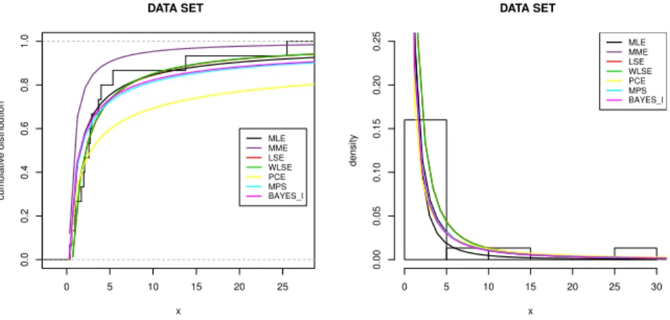
plotted in Figure 5. As we can see, it is a unimodal function. The Kolmogorov-Smirnov (K-S) distances between the fitted and empirical CDFs was 0.25, and the corresponding p-value was 0.22. Therefore, based on the MLEs, we can not reject the assumption that the data set are coming from the NP distribution.
We also computed K-S distance based on MMEs, LSEs, WLSEs, PCEs, MPSs and Bayes I estimates. Their estimates, K-S distances and the corresponding p-values are given in Table 6. From this table, all considered estimates provide a satisfactory to the data set. Table 7 presents 95% credible intervals.
Figure 6 plots the empirical CDF and histogram. Superimposed are the fitted CDFs and PDFs of the parameter estimates under consideration. These plots confirm the re-sults in Table 6.
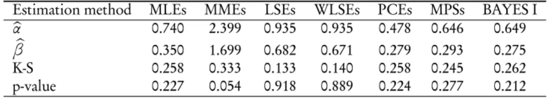
TABLE 6
Estimates, K-S distances and corresponding p-values based on different estimates for Example 1. Estimation method MLEs MMEs LSEs WLSEs PCEs MPSs BAYES I
b
α 0.740 2.399 0.935 0.935 0.478 0.646 0.649
b
β 0.350 1.699 0.682 0.671 0.279 0.293 0.275
K-S 0.258 0.333 0.133 0.140 0.258 0.245 0.262
p-value 0.227 0.054 0.918 0.889 0.224 0.277 0.212
TABLE 7
95%credible intervals of the parameters.
Parameter α β
10.2. Example 2 (βis known)
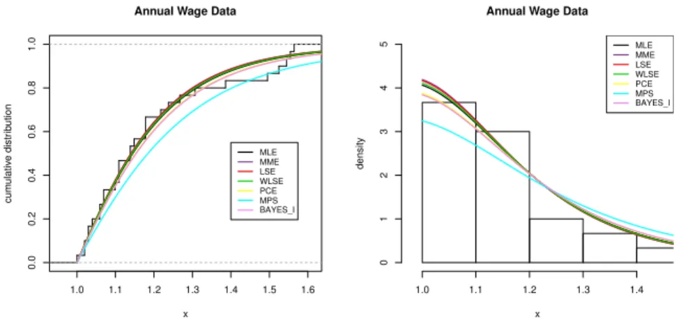
Dyer (1981) reported annual wage data (in multiplies of 100 US dollars) of a random sample of 30 production-line workers in a large industrial firm, as presented in Table 8. He showed that the Pareto distribution provided an adequate fit for this data set. Here we fit the NP distribution to this data set. We observed that the NP distribution withα=8.1261 andβ=101 fits to above data set. We checked the validity of the NP distribution based on the K-S test. The K-S distance was 0.09 and the corresponding p-value was 0.95. Let us transform this data set to the standard NP distribution with the scale parameterβ=1. We know that if the random variableX follows NP(α,β), then the random variableZ=X/βhas the standard NP(α, 1)distribution. Therefore, we transform the above data to NP(α, 1)by dividing byβ. The transformed data set are reported in Table 8.
We fitted the standard NP(α, 1)distribution to the transformed data set. We com-puted the MLE, MME, LSE, WLSE, PCE, MPS and Bayes I estimates ofαas described in Section 2. We also computed K-S distance based on these estimates. The estimates, K-S distances and the corresponding p-values are presented in Table 9. The results in Ta-ble 9 show that the standard NP(α, 1)model is fitted reasonably well to the transformed data set and all the estimates provide satisfactory fits. Table 10 presents 95% exact and asymptotic confidence intervals and also the 95% credible interval forα.
Figure 7 plots the empirical CDF and histogram. Superimposed are the fitted CDFs and PDFs of the parameter estimates under consideration. This figure supports the results in Table 9.
TABLE 8 The annual wage data.
Data Set 112 154 119 108 112 156 123 103
115 107 125 119 128 132 107 151
103 104 116 140 108 105 158 104
119 111 101 157 112 115
Transformed data 1.108 1.524 1.178 1.069 1.108 1.544 1.217 1.019 1.138 1.059 1.237 1.178 1.267 1.306 1.059 1.495 1.019 1.029 1.148 1.386 1.069 1.039 1.564 1.029 1.178 1.099 1.000 1.554 1.108 1.138
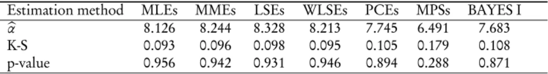
TABLE 9
Estimates, K-S distances and corresponding p-values based on different estimates for Example 2. Estimation method MLEs MMEs LSEs WLSEs PCEs MPSs BAYES I
b
α 8.126 8.244 8.328 8.213 7.745 6.491 7.683
K-S 0.093 0.096 0.098 0.095 0.105 0.179 0.108
TABLE 10
95% intervals ofαbased on the annual wage data.
Exact confidence interval Asymptotic confidence interval Credible interval
[5.887, 10.773] [5.971, 10.280] [6.117, 9.844]
11. CONCLUSIONS
We have compared eight methods to estimate parameters of a new Pareto distribution due to Bourguignonet al.(2016). Six of these are frequentist methods: maximum likeli-hood estimators, method of moment estimators, percentile estimators, least square and weighted least square estimators and maximum product of spacing estimators. The re-maining two are Bayes estimators based on informative and non-informative priors. The performance of the estimators was assessed by a simulation study and two real data ap-plications. The maximum product of spacing estimators and Bayes estimators based on informative priors were shown to provide the best performance when both parameters of the distribution are unknown. The percentile estimators and Bayes estimators based on informative priors were shown to provide the best performance when the scale pa-rameter of the distribution is known. A future work is to derive multivariate, matrix variate and complex variate extensions of the distribution and to study their estimation issues.
ACKNOWLEDGEMENTS
APPENDIX A. FIGURES
ε δ −100 −80 −80 −80 −60 −60 −40 −40 −20 −20 −20 −20 −20 −20 0 0 0 0 0 0 0 20 20 20 20
−0.04 −0.02 0.00 0.02 0.04
−0.04 −0.02 0.00 0.02 0.04 ε δ −60 −40 −40 −40 −40 −40 −40 −20 −20 −20 −20 −20 0 0 0 0 0
0 0
0 0 0 20 20 20 20 20
20 20
20 20 20 20 100 100
−0.04 −0.02 0.00 0.02 0.04
−0.04 −0.02 0.00 0.02 0.04 ε δ −500 −500 −500 0 0 0 0 0 0
0 0
0 0 0 0 0 500 1000
−0.04 −0.02 0.00 0.02 0.04
−0.04 −0.02 0.00 0.02 0.04 ε δ 0 0 0 0 0 0 0 0 0 0 0 0 1000 1000 1000 1000 1000 2000 2000 2000 7000
−0.04 −0.02 0.00 0.02 0.04
−0.04
−0.02
0.00
0.02
0.04
ε δ −1000 −100 −100 0 0 0 0 0 0 0 0 0 0 0 100 100 200 200
−0.04 −0.02 0.00 0.02 0.04
−0.04 −0.02 0.00 0.02 0.04 ε δ −50 0 0 0 0 0 0 0 0 0 0 0 0 0 50 50 50 50 50 50 100
100 100
−0.04 −0.02 0.00 0.02 0.04
−0.04 −0.02 0.00 0.02 0.04 ε δ −10000 0 0 0 0
0 0
0 0 0 5000 5000 10000
−0.04 −0.02 0.00 0.02 0.04
−0.04 −0.02 0.00 0.02 0.04 ε
δ 0
0 0 0 0 0 0 0 0 1e+05 1e+05 2e+05 3e+05 6e+05
−0.04 −0.02 0.00 0.02 0.04
−0.04
−0.02
0.00
0.02
0.04
ε δ −500 −100 −50 −50 −50 −50 −50 0 0 0 0 0 0 0 0 0 0 50 50 50 100 100
−0.04 −0.02 0.00 0.02 0.04
−0.04 −0.02 0.00 0.02 0.04 ε δ −70 −70 −60 −60 −50 −50
−40 −40
−30 −30 −30 −30 −30 −20 −20 −20 −20 −20 −20 −10 −10 −10 −10 −10 0 0 0 0 0 0 0 0 0 10 10 10 10 10 10 10 10 20 20 20 30
30 30 30
40 40 40 50 50 60 60 70 80
−0.04 −0.02 0.00 0.02 0.04
−0.04 −0.02 0.00 0.02 0.04 ε δ −8000 −8000 −4000 −2000 −2000
−2000 −2000
−2000 −2000 0 0 0 0 0 0 2000 4000 12000
−0.04 −0.02 0.00 0.02 0.04
−0.04 −0.02 0.00 0.02 0.04 ε
δ 0
0 0 0 0 1e+05 1e+05 1e+05 1e+05 1e+05 2e+05 2e+05 2e+05 8e+05
−0.04 −0.02 0.00 0.02 0.04
−0.04
−0.02
0.00
0.02
0.04
ε δ −1000 0 0 0 0 0 0 0 0 0 0 0 500 500 1000 1500
−0.04 −0.02 0.00 0.02 0.04
−0.04 −0.02 0.00 0.02 0.04 ε δ −60 −60 −60
−40 −40
−40 −40 −20 −20 −20 −20 −20 0 0 0 0 0 0 0 0 0 20 20 20 20 20 20 20 40 40 40 40 60
60 60
80 80 80 80 100 100 100 100 120 120 120 120 140 140 140 160 200 260
−0.04 −0.02 0.00 0.02 0.04
−0.04 −0.02 0.00 0.02 0.04 ε δ −28000 −18000 −16000 −16000 −10000 −6000 −4000 −2000 −2000 0 2000 2000 2000
−0.04 −0.02 0.00 0.02 0.04
−0.04 −0.02 0.00 0.02 0.04 ε
δ 0
0 0 0 0 5e+05 5e+05 5e+05 1e+06 1500000 1500000 2e+06 4500000 5e+06
−0.04 −0.02 0.00 0.02 0.04
−0.04
−0.02
0.00
0.02
0.04
0 1 2 3 4 5
−120
−100
−80
−60
−40
alpha
Profile log−lik
elihood
0.0 0.2 0.4 0.6 0.8 1.0
0.0
0.2
0.4
0.6
0.8
1.0
r/n
TT(r/n)
Figure 5 –Profile log-likelihood function ofα(left) and TTT plot for the data set (right).
0 5 10 15 20 25
0.0
0.2
0.4
0.6
0.8
1.0
DATA SET
x
cum
ulativ
e distr
ib
ution
MLE MME LSE WLSE PCE MPS BAYES_I
DATA SET
x
density
0 5 10 15 20 25 30
0.00
0.05
0.10
0.15
0.20
0.25 MLEMME
LSE WLSE PCE MPS BAYES_I
1.0 1.1 1.2 1.3 1.4 1.5 1.6
0.0
0.2
0.4
0.6
0.8
1.0
Annual Wage Data
x
cum
ulativ
e distr
ib
ution
MLE MME LSE WLSE PCE MPS BAYES_I
Annual Wage Data
x
density
1.0 1.1 1.2 1.3 1.4
0
1
2
3
4
5 MLE
MME LSE WLSE PCE MPS BAYES_I
Figure 7 –The empirical CDF and histogram with the fitted CDFs and PDFs.
REFERENCES
M. V. AARSET(1987).How to identify bathtub hazard rate. IEEE Transactions on Reli-ability, 36, pp. 106–108.
M. ABDI, A. ASGHARZADEH, H. S. BAKOUCH, Z. ALIPOUR(2019).A new compound gamma and Lindley distribution with application to failure data. Austrian Journal of Statistics, 48, pp. 54–75.
M. R. ALKASABEH, M. Z. RAQAB(2009).Estimation of the generalized logistic distribu-tion parameters: Comparative study. Statistical Methodology, 6, pp. 262–279.
B. C. ARNOLD (1983). Pareto Distributions. International Cooperative Publishing House, Fairland, Maryland, USA.
B. C. ARNOLD, S. J. PRESS(1983).Bayesian inference for Pareto populations. Journal of Econometrics, 21, pp. 287–306.
B. C. ARNOLD, S. J. PRESS(1989). Bayesian estimation and prediction for Pareto data. Journal of the American Statistical Association, 84, pp. 1079–1084.
A. ASGHARZADEH, R. REZAIE, M. ABDI(2011).Comparisons of methods of estimation for the half-logistic distribution. Selcuk Journal of Applied Mathematics, Special Issue, pp. 93–108.
M. BOURGUIGNON, H. SAULO, R. N. FERNANDEZ(2016). A new Pareto-type distri-bution with applications in reliability and income data. Physica A, 457, pp. 166–175.
M. H. CHEN, Q. M. SHAO(1999).Monte Carlo estimation of Bayesian credible and HPD intervals. Journal of Computational and Graphical Statistics, 8, pp. 69–92.
R. C. H. CHENG, N. A. K. AMIN(1979). Maximum product of spacings estimation with applications to the lognormal distribution. Tech. rep., Department of Mathematics, University of Wales.
R. C. H. CHENG, N. A. K. AMIN(1983).Estimating parameters in continuous univariate distributions with a shifted origin. Journal of the Royal Statistical Society, Series B, , no. 3, pp. 394–403.
C. DAGUM(2006). Wealth distribution models: Analysis and applications. Statistica, 66, no. 3, pp. 235–268.
R. DEMICHELI, G. BONADONNA, W. J. HRUSHESKY, M. W. RETSKY, P. VALAGUSSA (2004). Menopausal status dependence of the timing of breast cancer recurrence after sur-gical removal of the primary tumour. Breast Cancer Research, 6, no. 6, pp. 689–696.
S. DEY, T. DEY, D. KUNDU (2014). Two-parameter Rayleigh distribution: Different methods of estimation. American Journal of Mathematical and Management Sciences, 33, no. 1, pp. 55–74.
D. DYER(1981).Structural probability bounds for the strong Pareto laws. Canadian Jour-nal of Statistics, 9, pp. 71–77.
R. D. GUPTA, D. KUNDU(2001).Generalized exponential distribution: Different meth-ods of estimation. Journal of Statistical Computation and Simulation, 69, pp. 315–338.
N. L. JOHNSON, S. KOTZ, N. BALAKRISHNAN(1994). Continuous Univariate Distri-butions, vol. 1. Wiley, New York.
J. KAO(1959a).Computer methods for estimating Weibull parameters in reliability studies. IRE Transactions on Reliability and Quality Control, 13, pp. 15–22.
J. KAO(1959b).A graphical estimation of mixed Weibull parameters in life testing electron tubes. Technometrics, 1, pp. 389–407.
D. KUNDU, M. Z. RAQAB(2005). Generalized Rayleigh distribution: Different methods of estimation. Computational Statistics and Data Analysis, 49, no. 1, pp. 187–200.
C. LAI, M. XIE(2006). Stochastic Ageing and Dependence for Reliability. Springer, New York.
N. R. MANN, R. E. SCHAFER, N. D. SINGPURWALLA(1974). Methods for Statistical Analysis of Reliability and Life Data. Wiley, New York.
W. B. NELSON(1970). Statistical methods for accelerated life test data the inverse power law model. Technical report 71-c011, General Electric Company.
M. E. J. NEWMAN(2005). Pareto distributions and Zipfs law. Contemporary Physics, 46, no. 5, pp. 323–351.
V. PARETO(1964). Cours d’économie politique, vol. 1. Librairie Droz, Lausanne. B. RANNEBY(1984).The maximum spacing method, an estimation method related to the
maximum likelihood method. Scandinavian Journal of Statistics, 11, pp. 93–112.
P. G. SANKARAN, N. U. NAI, P. JOHN(2014).A family of bivariate Pareto distributions. Statistica, 74, no. 2, pp. 199–215.
J. SWAIN, S. VENKATRAMAN, J. WILSON(1988). Least squares estimation of distribu-tion funcdistribu-tion in Johnson’s transladistribu-tion system. Journal of Statistical Computadistribu-tion and Simulation, 29, pp. 271–297.
M. L. TIKU, A. D. AKKAYA(2004).Robust Estimation and Hypothesis Testing. New Age International (P) Limited, New Delhi.
L. ZANINETTI, M. FERRARO(2008). On the truncated Pareto distribution with applica-tions. Central European Journal of Physics, 6, no. 1, pp. 1–6.
SUMMARY
Bourguignonet al.(2016) introduced a new Pareto-type distribution to model income and reli-ability data. The aim of this paper is to estimate the parameters of this distribution from both frequentist and Bayesian view points. The maximum likelihood estimates, method of moment estimates, percentile estimates, least square and weighted least square estimates and maximum product of spacing estimates are considered as frequentist estimates. We have also considered the Bayes estimates of the unknown parameters and the associated credible intervals. The Bayes esti-mates are computed using an importance sampling method. To evaluate the performance of the different estimates, a Monte Carlo simulation study is carried out. Some real life data sets have been analyzed for illustrative purposes.
Keywords: Bayesian estimates; Least squares estimates; Maximum likelihood estimates; Method