Image Segmentation method based on Fuzzy
Clustering: Application to MR Brain Tissue
Extraction
Hanane Barrah
Laboratory of Innovative Technologies Abdelmalek Essaâdi University
Tangier, Morocco [email protected]
Abdeljabbar Cherkaoui
Laboratory of Innovative TechnologiesAbdelmalek Essaâdi University Tangier, Morocco [email protected]
Abstract—In this work, a fast and robust method for MR brain image segmentation is proposed. This method is based on a fast and robust fuzzy clustering algorithm that is initialized close to the searched solution in order to speed up the segmentation process. To validate the proposed method, we evaluate its performance on some grayscale images and on a normal brain (brought from the BrainWeb Simulated Brain Database). The experimental results are important in both robustness to noise and running times standpoints.
Keywords-MRI; c-means; fuzzy clustering; FCM; spatial information; segmetation.
I. INTRODUCTION
Magnetic resonance imaging (MRI) is a modern radiology technique that revolutionized the medical imaging world by allowing the exploration of the human body and many diseases. Several exploration axes derived from this imaging technique: Functional MRI (to study the brain functions), anatomical MRI (to visualize the brain tissues with a fine resolution), and diffusion MRI that is used to explore the brain areas connectivity.
To help physicians diagnose, study a tumor progression or make decisions, the processing and analysis of the MRI images has become necessary. Segmentation is a key component in assisting many radiological tasks, this is thanks to its role of extracting the most relevant information from an image such as points, shapes and regions.
To segment MR images, many segmentation methods have been developed [1], and each one depends on several factors such as the segmentation goal, image artifacts and noise types. Dzung L. Pham et al. published a survey about current medical image segmentation methods [1], in this work the authors focused on presenting the advantages and the drawbacks of each method in different imaging modalities including the MRI modality.
The most useful techniques in MRI image segmentation are based on the fuzzy clustering approach and more specifically
on the c-means algorithm [2]. Indeed, a wealth of work has been developed in this context. To extract brain tumors, Eman Abdel-Maksoud et al. [3] integrated the k-means algorithm with its fuzzy version c-means, in order to get benefits from their advantages, and used the median filter as a pre- and post-processing to remove noise. As a pre-post-processing method, the median filter presents two main problems. The first one is increasing the computational time, while the second one lies on the loss of some fine details [4], which alters the clustering quality in a negative way. To get over this latter limitation and increase the efficiency of the c-means algorithm in presence of noise, several researchers improved it in many ways. the majority tried to include the filtering step in the clustering process by integrating spatial information, while the rest tried to modify the dissimilarity measure.
To overcome the sensitivity to noise and other imaging artifacts, Dzung L. Pham [5] extended the c-means algorithm by incorporating a spatial penalty term in the objective function. Even though this extended algorithm showed its accuracy over other competing approaches, it still suffers from two major problems. The first one is the difficult selection of the parameter that controls the effect of the penalty term, and the second problem is its time requirement.
To improve its efficiency, robustness to noise and processing speed, and make it suitable for extracting non-Euclidean structures, the FCM_S algorithm [6] was extended to five other variants by S. Chen and D. Zhang [7]. The main idea of S. Chen and D. Zhangs’ work is based on including the median (or mean) filter into the clustering process and using kernel methods.
J. Wang et al. [8] proposed a modified c-means algorithm based on a modified distance measurement that incorporates both local and non-local information.
problem and make these algorithms fully free of the empirical parameters, we introduced in [9] a new factor, based on the local spatial and the gray level information, that is automatically adjustable. The strength of the extended algorithms was demonstrated on synthetic and real images.
The aim of this work is centered on providing a fast and robust segmentation method for MR brain images. To this end, the main ideas of the algorithms presented in [9] and [10] are used to develop a Fast RFCMLGI (Robust FCM with Local and Gray Information) algorithm, which is also incorporated into a method that initializes the fuzzy clustering algorithm close to the searched solution and refines the clustering results.
The rest of this article is structured as follows: In section 2 are presented the conventional FCM and the algorithms developed in [9]. The proposed method is described in section 3. Section 4 is dedicated for some experimental results and comparisons. In section 5, we conclude by some remarks and perspectives.
II. FUZZY CLUSTERING
A. Conventinal FCM
C-means or FCM [11], [12] is the well-known fuzzy clustering algorithm that consists of grouping pixels into the most homogeneous groups by minimizing iteratively the objective function (1).
(
)
C N m 2j i ij i=1 j=1
.
J D, U, C
=
u . x c− (1)Where D is the input data, U= uij is the fuzzy partition
matrix that satisfies the condition (2), C is the set of the cluster
centers,
.
is the Euclidean distance, and m is the fuzzinessexponent that is always chosen equal to 2 [13]:
c Nij ij ij
i 1 j 1
u 0,1 u 1, j and 0 u N, i .
= = =
(2)The membership values and the cluster centers are updated as follows:
-2 C -2
m-1 m-1
ij j i j k
k=1
=
u
x - c
x - c
.
(3)N N
m m
i ij j ij
j 1 j 1
c
u .x
u
.
= =
=
(4)B. Robust FCM with Local and Gray Information: RFCMLGI
The major drawback of the conventional FCM algorithm lies on the lack of spatial information, which makes it very sensitive to noise and outliers. To overcome this problem, the FCM algorithm has been modified in many ways [5]–[8], [14]. However, most of its extensions require the adjustment of some empirical parameters such as α in [7]. In order to make the FCM algorithm robust to noise and automatic, we introduced in our earlier work [9] a new factor S (defined in (5)) that includes the local spatial and the gray level information. The objective function based on S is defined as in (6):
j
j r j
Rr N rj
x x
1
S .
N d 1
− =
+
(5)NR and Ni are defined as in the FCM_S, and drj represents
the spatial Euclidean distance between the pixels xj and xr.
(
)
j
C N m 2
j i ij i=1 j=1
C N m ij j i=1 j=1
R r N
. c
1 2
. . xr ci .
N
J D, U, C u x
S u
=
− + − (6)The algorithm that minimizes (6) using (7) and (8) is called Robust FCM with Local and Gray Information (RFCMLGI).
( ) ( ) j j 1 m 1
2 j 2
j i r i
R r N
1 m 1
C 2 j 2
j k r k
R
k 1 r N
S N . ij S N
x c x c
u
x c x c
− − − − = − + − = − + −
(7)(
)
j N j mij j r
R
j 1 r N
i N m j ij j 1 S N
u . x x
c
1 S .u
= = + = + (8)
In order to speed up the clustering process, the objective function (6) has been extended to the following one (9), which leads us to two other versions of the RFCMLGI algorithm, RFCMLGI_1 and RFCMLGI_2 that updatethe partition matrix and the cluster centers using (10) and (11) respectively.
(
)
C N 2 C N 2m m
j i j i
ij j ij
i=1 j=1 i=1 j=1
c . c
J D, U, C
=
u . x−+
S u . x − (9)(
)
( )(
)
( )1
2 2 m 1
j i j j i
ij 1
C 2 2 m 1
j k j j k
k 1
x c S x c
u
x c S x c
− − − − = − + − = − + − (10)
(
)
(
)
N mij j j j j 1
i N
m j ij j 1
u . x S .x c
1 S .u
= = + = + (11) j
x could be the mean or the median value of the neighbors
within a specified window aroundxj.
III. THE PROPOSED METHOD
Our algorithms presented in [9] proved their robustness to noise on grayscale images. Thus, they could perform in a similar manner on MRI data, as they are also grayscale images. In this paper we improved them, in terms of speed, and incorporated them into a fast and robust MR brain image segmentation method, that aims to extract the three main brain tissues: white matter (WM), gray matter (GM) and cerebrospinal fluid (CSF).
A. Speed improvement of RFCMLGI
The spatial information introduced in the objective functions (6) and (9) via a neighborhood term appears in the updating equations (7), (8), (10) and (11). Which means that this term has to be computed in each iteration, which requires the algorithm to perform slower. To overcome this problem, we adopted the idea of Jiu-Lun Fan et al. [10]. Actually, we modified our algorithm RFCMLGI and its variants by introducing a parameter γ that controls the trade-off between the fastness of the hard clustering algorithm and the robustness of RFCMLGI (and its variants) to noise. The idea behind Jiu-Lun Fan’s algorithm is to prize the biggest membership degree and suppress the others.
Let xj be a pixel and ubj be its degree of belongingness to the
bth cluster. If u
bj is the biggest value of all the clusters, then the
membership degrees of xj will be modified as follows:
bj ij bj
i b
u = 1- γ. u = 1- γ + γ.u
(12)
ij ij
u = γ.u , ib (13)
Where
0, 1 . When gets closer to 0, the algorithm becomes more hard and when it approaches 1 the algorithm tends to the fuzzy version. According to Jiu-Lun Fan et al., 0.5 is a better value for γ when there is no information about the data structure.This modification has to be done immediately after updating the fuzzy partition matrix. Thus, we come up with the following algorithm that is slightly different from the previous one RFCMLGI.
Fast_RFCMLGI Algorithm
• Fix the clustering parameters (the converging error , the fuzziness exponent m and the number of clusters C), input the dataset D, initialize randomly the cluster centers and the parameter γ.
• Compute S using (5).
• Repeat
1. Update U using (7).
2. Modify U using (12) and (13). 3. Update C using (8).
• Until Unew−Uold
B. Clustering result refinement
Mathematical morphology based methods are interested on analyzing geometrical structures. They consist of using a structuring element (small shape) and performing a series of basic and complex operations (dilations, erosions, opening and closing) in order to achieve the desired segmentation. These methods can be used to segment an image or to improve the segmentation result of another method. To learn about this important topic, relevant publications are available [15]–[18].
In this work, we use the closing operation in the post-processing stage in order to improve the clustering result quality. The closing operation is a dilation followed by an erosion using the same structuring element, which leads to filling black holes and merging close regions of the same cluster. Actually, the dilation process consists of expanding the objects borders (white regions on a black background), while the erosion is defined as the opposite operation that consists of shrinking the objects sizes. This last operation ends up by removing objects with sizes smaller than that of the structuring element.
C. The proposed method
To segment a single MR image, the Fast_RFCMLGI algorithm and its variants are sufficient in terms of accuracy and computational time. However, in case of segmenting a series of images, the segmentation process becomes heavier. This problem is mainly due to the big size of data and the random initialization of the fuzzy clustering algorithm. In fact, when the clusters centers are initialized randomly, they can be localized far from the searched ones, which requires the algorithm to perform slowly. To overcome this problem, we propose a method that processes the volume slices in a sequential order. At first, it takes as input a series of MR images and segments the first slice using a random initialization. To segment any other slice of the volume, the proposed method uses the clustering result of the previous slice to initialize the clustering algorithm Fast_RFCMLGI. In this way, the algorithm is initialized close to the search solution, which allows it to converge faster. In fact, it is obvious and well known that two consecutive MR brain slices are very similar in terms of structures, shapes and matters (WM, GM and CSF), which means that their clustering results are very close.
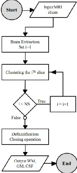
Fig. 1. Steps of the proposed method
Fig. 1 illustrates the method steps from the input to the output. NS is the constant that refers to the total number of slices and i is the variable used to test whether the last slice is achieved or not. The MRI slices are numbered from one (the lowest slice) to NS (the superior slice).
• Brain extraction: This step is primordial in any MR brain image segmentation method because it reduces the data size and the clusters number. It consists of removing non-brain structures such as skin, eyeballs, skull, fat and muscle. In this work, we use the Brain Extraction Tool (BET) developed by Stephen M. Smith [19].
• Clustering the iTh slice: If i is equal to 1, then the first
slice is partitioned using a random initialization. Otherwise, if 1 < i ≤ NS, then the iTh slice is partitioned
using the clustering result of the (i-1)Th slice as an
initialization of the Fast_RFCMLGI algorithm.
• Defuzzification: In this step, the WM, GM and CSF masks are extracted from the partition matrices U using a defuzzification process (each pixel is assigned to the cluster where the membership value is the biggest one). To improve the clustering result, a closing operation is performed on each binary card.
IV. EXPERIMENTAL RESULTS
To show the efficiency of the proposed method, we compare it with the conventional FCM and RFCMLGI. The clustering parameters were fixed as: m=2 [13], ɛ=10-8 and γ=0.5 [10].
The structuring element used is a 2D diamond-shape with a radius equal to 1.
The algorithms (FCM and RFCMLGI) and the proposed method are implemented in Matlab R2016b and tested on an Intel Core i7 (4.4 GHz) computer under Windows 7.
This section contains two main subsections. In the first one are presented the results on some grayscale images, while in the second subsection are depicted the results on some series of MRI images.
A. Grayscale images
The proposed method, FCM and RFCMLGI are applied on a synthetic and three real grayscale images (See Fig. 2) that are corrupted by Gaussian and ‘Salt&Pepper’ noise.
Fig. 2. Test images. (a) Synthetic. (b) Moon. (c) Elephant. (d) Wolf.
1) Synthetic Image. The synthetic image contains 255 255 pixels spanning into two classes with two gray levels taken as 200 and 50. To measure the performance of the proposed method and that of each fuzzy clustering algorithm on the synthetic image, we used the Segmentation Accuracy (SA) defined as follows:
Number of correctly classified pixels SA
Total number of pixels
=
Visual results are shown in Fig. 3 and Fig. 4, while the segmentation accuracies and the running times are depicted Table. 1 and Table. 2 respectively.
that the proposed method performed faster than the RFCMLGI algorithm. Thus, the proposed method achieved better result within a reasonable time.
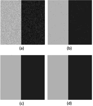
Fig. 3. Segmentation results on the Synthetic image. (a) image corrupted by Gaussian noise. (b) FCM result. (c) RFCMLGI result. (d) Result of the proposed method.
Fig. 4. Segmentation results on the Synthetic image. (a) image corrupted by ‘Salt & pepper’ noise. (b) FCM result. (c) RFCMLGI result. (d) Result of the proposed method.
Table. 1 Segmentation accuracies (SA in %) obtained on the synthetic image
Algorithms
Noise Type
FCM RFCMLGI Proposed Method
Gaussian noise 99.85 100 100
Salt&Pepper noise 97.57 99.95 100
Table. 2 Running times (in seconds) performed on the synthetic image
Algorithms
Noise Type
FCM RFCMLGI Proposed Method
Gaussian noise 0.45 7.76 3.09
Salt&Pepper noise 0.39 15.39 6.58
2) Moon Image. (356×536 pixels in size) This image was used in [9] to prove the robustness of the RFCMLGIalgorithm and its two variants. The image was corrupted at the same time by Gaussian and ‘Salt & Pepper’ noise. In this experiment, C is fixed to 2. Visual results are presented in Fig. 5, while the number of iterations and the running times performed are summarized in Table. 3 and Table. 4 respectively.
Fig.5. Segmentation results on the Moon image. (a) image corrupted by Gaussian and ‘Salt & pepper’ noise. (b) FCM result. (c) RFCMLGI result. (d) Result of the proposed method.
From Fig. 5, we notice that the conventional FCM provided the worst segmentation, where it could not deal with noisy pixels. However, the RFCMLGI algorithm and the proposed method succeeded ,to different extent, to handle noise. In fact, the proposed method provided the best segmentation result, where it corrected some noisy pixels that appear in the RFCMLGI result, especially at the image borders and inside the regions circled in gray.
In terms of speed, from Table. 3, we remark that the proposed method performed less iterations than the RFCMLGI algorithm, which is also reflected by the running times depicted in Table. 4. Actually, the proposed method performed faster.
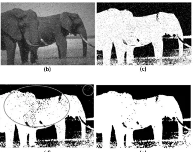
3) Elephant Image. (481×321 pixels in size) To confirm the remarks of the previous results, we performed some experiments on the Elephant[20] image corrupted by Gaussian and ‘Salt & Pepper’ noise respectively. In each experiment, C is fixed to 2. Visual results are presented in Fig. 6 and Fig. 7, while the numbers of iterations and the running times performed are summarized in Table. 3 and Table. 4 respectively.
As previously, from Fig. 6 and Fig. 7, we observe that the conventional FCM failed to handle noisy pixels, while the proposed method provided the best segmentation results. In fact, noisy pixels at the image borders (appear in the RFCMLGI results) and inside the regions circled in gray are corrected by the proposed method.
From Table. 3 and Table. 4, we remark that the proposed method required less iterations and performed faster than the RFCMLGI algorithm.
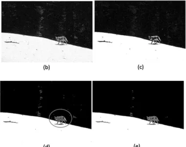
4) Wolf Image. (481×321 pixels in size) In the previous experiments we tried to extract one object (one cluster) from the background, that is why we fixed C to 2. This time, the efficiency of the proposed method is demonstrated on the Wolf [20] image that contains three main clusters (forest, wolf and ground), thus, C is fixed to 3. The experiments were performed on the image corrupted by Gaussian and ‘Salt & Pepper’ noise respectively. Visual results are presented in Fig. 8 and Fig. 9, while the numbers of iterations and the running times performed are summarized in Table. 3 and Table. 4 respectively
From Fig. 8 and Fig. 9, it is clearly noticeable that the results of the FCM algorithm are the worst and those of the proposed method are the best ones. As previously, noisy pixels that appear in the RFCMLGI results, especially at the image borders and inside the regions circled in gray, are corrected by the proposed method.
From Table. 3 and Table. 4, we see that our method required less iterations and performed faster than the RFCMLGI algorithm.
According to the remarks drawn from all the experiments on the grayscale images, we conclude that the proposed method is:
• Fast: The parameter γ helps to reduce the number of iterations, and consequently decrease the running times.
• Robust: This property is obtained, first from the spatial information introduced in the objective function, and second from the closing operation.
Fig. 6. Segmentation results on the Elephant image. (a) image corrupted by Gaussian noise. (b) FCM result. (c) RFCMLGI result. (d) Result of the proposed method.
Fig. 7. Segmentation results on the Elephant image. (a) image corrupted by Salt & Pepper noise. (b) FCM result. (c) RFCMLGI result. (d) Result of the proposed method.
Fig. 8. Segmentation results on the Wolf image. (a) Original image. (b) image corrupted by Gaussian noise. (c) FCM result. (d) RFCMLGI result. (e) Result of the proposed method.
Fig. 9. Segmentation results on the Wolf image. (a) Original image. (b) image corrupted by Salt & Pepper noise. (c) FCM result. (d) RFCMLGI result. (e) Result of the proposed method.
Table. 3. Number of iterations performed by RFCMLGI and the proposed method
Images RFCMLGI Proposed Method
Moon with mixed noise 27 17
Elephant
Gaussian noise 38 21
Salt & Pepper noise 39 25
Wolf
Gaussian noise 98 22
Salt & Pepper noise 42 27
Table. 4. Running times (in seconds) performed by RFCMLGI and the proposed method
Images RFCMLGI Proposed Method
Moon with mixed noise 54,3 33
Elephant
Gaussian noise 56,14 31,5
Salt & Pepper noise 58,14 32,7
Wolf
Gaussian noise 246,06 50
Salt & Pepper noise 88,6 60,7
B. MR images
In order to see how the initialization of the clustering algorithm affects the convergence speed of our method, we examine its performance on seven series of MR images. In each experiment, we increase the number of the input images, run the Fast_RFCMLGI algorithm with the random initialization (and with the proposed initialization respectively) five times on each dataset and calculate the mean time in each case. The MR images used in these experiments are simulated using the BrainWeb Simulated Brain Database [21].
The running times required by the Fast_RFCMLGI with the random initialization (and with the proposed initialization respectively) are presented in Fig. 10. The black line (Random_In) refers to the running times required by the Fast_RFCMLGI algorithm with the random initialization, while the gray line (Proposed_In) refers to those required by the same algorithm based the initialization proposed in the previous section.
From Fig. 10, it is clearly noticeable that the running times Random_In and Proposed_In increase as the number of the input images increases, which is reasonable. Moreover, the Fast_RFCMLGI with the proposed initialization performed faster than using random initialization. This is due to the initialization of the algorithm close to the searched solutions, which allows it to make less iterations and consequently converge rapidly.
Fig. 10. Running times reqired by the RFCMLGI_2 algorithm
The numbers of iterations and the running times required to partition each slice of the fifth dataset (composed of 10 images 86-95) are depicted in Table 5.
From Table 5, we see that the Fast_RFCMLGI algorithm based on the random initialization required more numbers of iterations and running times to segment each slice, which leads to a total running time (3 minutes and 38 seconds) that is bigger than that performed by the same algorithm based on the proposed initialization (2 minutes and 36 seconds).
From the experimental results presented in this subsection, we conclude that the proposed initialization helps to dramatically decrease the running times required to segment a series of brain MR images.
In terms of shape, the real grayscale images used before are less complex than the MR brain images used in the last subsection. However, the first ones required more running times (between 31.5 and 60.7 seconds). Actually, the MR images slice86-slice95 required less running times (between 12 and 22.66 seconds), this is owing to the proposed initialization: for each slice (from slice87 to slice95), the clustering algorithm is initialized by the segmentation result of the previous slice.
V. CONCLUSION
In the aim of providing a fast and robust segmentation method for MR brain images, we improved our automatic algorithm RFCMLGI, in terms of speed, and focused on the initialization step. In fact, we proposed to initialize the clustering algorithm close to the searched solution in order to speed up the algorithm convergence, and thus reduce the computational time. By testing this method on some grayscale images and on a normal brain, we noticed its fastness and robustness to noise.
In light of these valuable results, two main perspectives will be studied in the future. First, improve the proposed segmentation method in order to extract brain tumors and/or lesions. In this context, a combination of the proposed method with a contour-based method, such as Active Shape Model (ASM), is essential in order to delineate the boundaries between normal (WM, GM and CSF) and abnormal (tumors and lesions) structures. Second, because of the big size of data (3D MR images), it is important to parallelize the computations and data, and make a better use of the material resources in order to speed up the segmentation process.
Table. 5. Experimental results on the 5Th dataset
Slice Original images The proposed method results
Number on iterations Running times (in seconds)
Random Initialization
Proposed Initialization
Random Initialization
Proposed Initialization
86 34 34 23 22.66
87 35 17 25 12.9
88 33 19 22.24 13.43
Slice Original images The proposed method results
Number on iterations Running times (in seconds)
Random Initialization
Proposed Initialization
Random Initialization
Proposed Initialization
89 33 26 22.27 17.75
90 33 21 22.59 14.53
91 30 21 19.88 14.96
92 34 25 22.45 17.72
93 30 20 20 13.92
Slice Original images The proposed method results
Number on iterations Running times (in seconds)
Random Initialization
Proposed Initialization
Random Initialization
Proposed Initialization
94 30 17 20.54 12
95 30 25 20.69 17
Total Running times 3min 38s 2min 36s
REFERENCES
[1] D. L. Pham, C. Xu, et J. L. Prince, « Current methods in medical image segmentation 1 », Annu. Rev. Biomed. Eng., vol. 2, no 1, p. 315–337, 2000.
[2] J. C. Bezdek, Fuzzy models and algorithms for pattern recognition and image processing. New York: Springer, 2005.
[3] E. Abdel-Maksoud, M. Elmogy, et R. Al-Awadi, « Brain tumor segmentation based on a hybrid clustering technique », Egypt. Inform. J., vol. 16, no 1, p. 71‑81,
mars 2015.
[4] A. B. Hamza, P. L. Luque-Escamilla, J. Martínez-Aroza, et R. Román-Roldán, « Removing noise and preserving details with relaxed median filters », J. Math. Imaging Vis., vol. 11, no 2, p. 161–177, 1999.
[5] D. Pham, « Spatial Models for Fuzzy Clustering »,
Comput. Vis. Image Underst., vol. 84, no 2, p. 285‑297,
nov. 2001.
[6] M. N. Ahmed, S. M. Yamany, N. Mohamed, A. A. Farag, et T. Moriarty, « A modified fuzzy c-means algorithm for bias field estimation and segmentation of MRI data »,
Med. Imaging IEEE Trans. On, vol. 21, no 3, p. 193–199,
2002.
[7] S. Chen et D. Zhang, « Robust Image Segmentation Using FCM With Spatial Constraints Based on New Kernel-Induced Distance Measure », IEEE Trans. Syst. Man Cybern. Part B Cybern., vol. 34, no 4, p. 1907‑1916,
août 2004.
[8] J. Wang, J. Kong, Y. Lu, M. Qi, et B. Zhang, « A modified FCM algorithm for MRI brain image segmentation using both local and non-local spatial constraints », Comput. Med. Imaging Graph., vol. 32, no
8, p. 685‑698, déc. 2008.
[9] H. Barrah, A. Cherkaoui, et D. Sarsri, « Robust FCM Algorithm with Local and Gray Information for Image Segmentation », Adv. Fuzzy Syst., vol. 2016, p. 1‑10, 2016.
[10] J.-L. Fan, W.-Z. Zhen, et W.-X. Xie, « Suppressed fuzzy c-means clustering algorithm », Pattern Recognit. Lett., vol. 24, no 9‑10, p. 1607‑1612, juin 2003.
[11] L. Rokach et O. Maimon, « Clustering methods », in
Data mining and knowledge discovery handbook, Springer, 2005, p. 321–352.
[12] D. Lam et D. C. Wunsch, « Chapter 20 - Clustering », in
Academic Press Library in Signal Processing, vol. Volume 1, J. A. K. S. Paulo S.R. Diniz Rama Chellappa and Sergios Theodoridis, Éd. Elsevier, 2014, p. 1115‑ 1149.
[13] I. Ozkan et I. B. Turksen, « Upper and lower values for the level of fuzziness in FCM », Inf. Sci., vol. 177, no 23,
p. 5143‑5152, déc. 2007.
[14] L. Szilagyi, Z. Benyo, S. M. Szilágyi, et H. S. Adam, « MR brain image segmentation using an enhanced fuzzy c-means algorithm », in Engineering in Medicine and Biology Society, 2003. Proceedings of the 25th Annual International Conference of the IEEE, 2003, vol. 1, p. 724–726.
[15] J. Serra, « Introduction to mathematical morphology »,
Comput. Vis. Graph. Image Process., vol. 35, no 3, p.
283–305, 1986.
[16] V. Ćurić, A. Landström, M. J. Thurley, et C. L. Luengo Hendriks, « Adaptive mathematical morphology – A survey of the field », Pattern Recognit. Lett., vol. 47, p. 18‑28, oct. 2014.
[17] J. Serra, « Morphological filtering: An overview », Signal Process., vol. 38, no 1, p. 3‑11, 1994.
[18] L. Vincent, « Morphological grayscale reconstruction in image analysis: applications and efficient algorithms »,
IEEE Trans. Image Process., vol. 2, no 2, p. 176–201,
1993.
[19] S. M. Smith, « Fast robust automated brain extraction »,
Hum. Brain Mapp., vol. 17, no 3, p. 143–155, 2002.
[20] D. Martin, C. Fowlkes, D. Tal, et J. Malik, « A database of human segmented natural images and its application to evaluating segmentation algorithms and measuring ecological statistics », in Computer Vision, 2001. ICCV 2001. Proceedings. Eighth IEEE International Conference on, 2001, vol. 2, p. 416–423.
[21] C. A. Cocosco, V. Kollokian, R. K.-S. Kwan, G. B. Pike, et A. C. Evans, « BrainWeb: Online Interface to a 3D MRI Simulated Brain Database », NeuroImage, vol. 5, p. 425, 1997.