Numerical Solution of Two Dimensional Fredholm Integral Equations of the Second Kind by the Barycentric Lagrange Function*

ISSN Online: 2327-4379 ISSN Print: 2327-4352

DOI: 10.4236/jamp.2017.52023 February 15, 2017

Numerical Solution of Two Dimensional

Fredholm Integral Equations of the Second

Kind by the Barycentric Lagrange Function

*

Hongyan Liu, Jin Huang, Yubin Pan

School of Mathematical sciences, University of Electronic Science and Technology of China, Chengdu, China

Abstract

This paper solves the two dimensional linear Fredholm integral equations of the second kind by combining the meshless barycentric Lagrange interpola-tion funcinterpola-tions and the Gauss-Legendre quadrature formula. Inspired by this thought, we convert the equations into the associated algebraic equations. The results of the numerical examples are given to illustrate that the approximated method is feasible and efficient.

Keywords

Two Dimensional Fredholm Integral Equations, Barycentric Lagrange Interpolation Functions, Gauss-Legendre Quadrature Formula

1. Introduction

Many of the mathematical physics problems and the engineering problems can be transformed into solving Fredholm integral equations [1] [2] [3]. In this pa-per, we pay attention to the two dimensional linear Fredholm integral equations (FIEs) of the second kind

( ) ( )

, ,

( ) ( )

, , b d

(

, ; ,

) ( )

, d d ,

( )

, ,

a c

a x y u x y = f x y +b x y

∫ ∫

k x y s t u s t s t x y ∈Ω (1) where a x y

( ) ( )

, ,b x y, and f x y

( )

, are non-zero continuous functions on the

bounded region Ω =

[ ] [ ]

a b, × c d, , and the kernel function

(

, ; ,

)

(

)

k x y s t ∈C Ω×Ω , u x y

( )

, is the undetermined function. Usually, it’s

dif-ficult to obtain the analytic solutions of integral equations, so the numerical so-lutions of the integral equations are necessarily needed.

There are some researches for obtaining the numerical solutions of two

di-*This work was supported by the National Natural Science Foundation of China (11371079). How to cite this paper: Liu, H.Y., Huang,

J. and Pan, Y.B. (2017) Numerical Solution of Two Dimensional Fredholm Integral Equations of the Second Kind by the Bary-centric Lagrange Function. Journal of Ap-plied Mathematics and Physics, 5, 259-266. https://doi.org/10.4236/jamp.2017.52023

mensional FIEs, such as the radial basis functions method [4], Haar wavelets [5] and integral mean value method [6] [7]. Berrut specializes the barycentric La-grangian interpolation formula [8], and some other authors present the corres-ponding numerical stability analyses in the literatures [9] [10] [11]. The authors take advantage of the equally spaced barycentric Lagrange polynomial to solve one dimensional linear Volterra-Fredholm integro-differential equations in [12]. There exists an intrinsic problem that polynomial interpolation is ill-posed at the equispaced nodes. This paper presents a modified Lagrange interpolation me-thod with Chebyshev nodes to solve two dimensional linear Fredholm integral equations of the second kind.

This paper is constructed as follows: Section 2, we display the barycentric in-terpolation function. Section 3, we transform the two dimensional FIEs into the algebraic equations by utilizing the barycentric function and the composite Gauss- Legendre quadrature formula. Section 4, the numerical examples illustrate the efficiency and applicability of our method via comparing with the Lagrange me-thod.

2. Barycentric Interpolation Function

Barycentric Lagrange interpolation function (BLIF) is a variant of Lagrange in-terpolation function (LIF).

2.1. One Dimensional Barycentric Interpolation Function

The one dimensional barycentric Lagrange formula about continuous function

( )

,

[ ]

,

u x x∈ a b at the nodes a=x0 ≤x1≤ … ≤xn =b is introduced as

0 ( ) ( ) ,

n

n j j

j

u x L x u

=

=

∑

₍₂₎ where u_j =u x

( )

_j , j=0,1,…,n are the function values of u x

( )

, and L_j

( )

x are the barycetric Lagrange interpolation basis functions

( )

0

, 0,1, , ,

n

j k

j

k

j k

w w

L x j n

x x = x x

   

=_{ −}  _{ −}  =

 

 

∑

 (3)

which satisfy the property Lj

( )

xi =δij, where δij is the Kronecker-delta

func-tions. And wj are the barycentric interpolation weight functions

(

)

0,

1 ,

n

j j k

j j k

w x x

= ≠

 

= _ − _



∏

 (4)

and wj only depend on the distribution of nodes.

The barycentric Lagrange interpolation formula is stable forward when we choose the Chebyshev points as interpolating points [9]. At the same time, the weight functions are simplified as w_j = −

( )

1 jξ_j, where 1

2

j

ξ = for j=0,m

and ξ_j =1 for j≠0,m.

2.2. Two Dimensional Barycentric Interpolation Function

dimensional barycentric Lagrange interpolation function about a continuous function u x y

( ) ( )

, , x y, ∈

[ ] [ ]

a b, × c d, as follows

( )

( )

0 0

, , ,

m n

mn ij ij

i j

u x y L x y u

= =

=

∑∑

₍₅₎

where uij=u x y

(

i, j

)

, and the tensor product points

(

x yi, j

)

are obtained by

subdividing

[ ]

a b, and

[ ]

c d, into the calculation nodes 0 1 m

a=x <x <<x =b and c=x0<x1<<xn=d, respectively. The two

dimensional barycentric interpolation basis functions L_ij

(

x y,

)

satisfy

(

,

)

( ) ( )

,

ij i j

L x y =L x L y (6) where L xi

( )

and Lj

( )

y are equal to (4). The above equation has the

follow-ing property

(

)

1, and ,

,

0, others.

ij k l

i k j l L x y =  = =

 (7)

In the practical calculation, we take the second Chebyshev nodes

(

x y_i, _j

)

,

cos π i i x m   = − _{ }

 , i=0,1,,m, j cos π

j y

n

 

= − _{ }

 , j=0,1,,n as the interpo-lation nodes.

3. The Barycentric Method of Two Dimensional Fredholm

Integral Equation

We enter (5) into (1) to approximate two dimensional Fredholm integral equa-tion

( )

( )

( ) ( )

(

)

( )

0 0 0 0 , ,

, , , ; , , d d ,

m n ij ij i j m n b d ij ij a c i j

a x y L x y u

f x y b x y k x y s t L s t u s t

= =

= =

= +

∑∑

∑∑

∫ ∫

(8)

then taking the collocation points

(

x yk, l

)

into (8), and exchanging the integral

and summation sign

(

)

(

)

(

) (

)

(

) ( )

0 0

0 0

, ,

, , , ; , , d d .

m n

k l ij k l ij i j

m n b d

k l k l _{a c} k l ij ij

i j

a x y L x y u

f x y b x y k x y s t L s t s t u

= = = =   = + _{ }  

∑∑

∑∑ ∫ ∫

(9)

Now, we deal with the integral part and let

2 2

b a b a

s= + + − σ and

2 2

c d d c

t= + + − τ, then we can easily have

(

) ( )

1 1

(

)

(

)

1 1,

1 1

, ; , , d d d , ; , , d ,

b d

k l ij k l ij

a ck x y s t L s t s t= − σ −k x y σ τ L σ τ τ

∫ ∫

∫

∫

(10)

where 1

(

, ; ,

)

, ; ,

2 2 2 2 2 2

k l k l

b a d c a b b a c d d c

k x y σ τ = − − k x y_ + + − σ + + − τ_

 ,

(

)

1, , ,

2 2 2 2

ij ij

a b b a c d d c

L =L σ τ _ + + − σ + + − τ_

Gauss-Legendre quadrature formula to approximate integral (10). Then the Eq-uation (9) becomes

(

) (

) (

)

(

) (

)

(

)

1 1,

0 0 1 1

, , , , ; , ,

, ,

m n M N

k l ij k l k l p q k l p q ij p q ij

i j p q

k l

a x y L x y b x y l l k x y L u

f x y

σ τ σ τ

= = = =

 

−

 

 

=

∑∑

∑∑

₍₁₁₎

where l_p,l_q; σ τ_p, _q are the quadrature coefficients and points of the compo-site Gauss-Legendre quadrature formula, respectively. Finally, we transform the Equation (1) into algebraic equations. The solution of the Equation (11) is close to (1). The whole process is called discrete collocation method whose nature is the Nyström iterative approach. We can analyze the existence, uniqueness and convergence of the approximate solution under the theoretical framework of the Nyström from [13]. Once we obtain uij, we can get the values of the discrete

collocation solution u x y

( )

, at any interior points.

The specific Algorithm is as follows

Step 1: Construct two dimensional Chebyshev nodes

(

x y_i, _j

)

,

cos

i

i x

mπ

 

= − _{ }

 , j cos

j y

nπ

 

= − _{ }

 ,

Step 2: Approximate integral operator K in (10) by using composite Gauss- Legendre quadrature formula,

Step 3: Solve the algebraic Equations (11) using the above steps and Gaussian elimination method.

4. Numerical Example

In this section, we present two numerical examples to verify the effectiveness and accuracy of the barycentric method. Defining the absolute error (AE) and the relative error (RE) as

( )

,

( )

, _mn

( )

, ,

e x y = u x y −u x y (12)

( )

,

( )

,

_{( )}

( )

, ,

,

mn

u x y u x y

re x y

u x y

−

= ₍₁₃₎

and u x y

( )

, , umn

( )

x y, represent the exact and approximate solution of Equa-

tion (1), respectively.

Example 1. For the following two dimensional linear Fredholm integral equa-tion of the second kind

( )

(

)

1 1

( )

( ) ( )

[ ] [ ]

0 0

, sin , d d , , , 0,1 0,1 ,

u x y = x+y

∫ ∫

u s t t s+ f x y x y ∈ × (14) where f x y

( )

, = +_1 sin 2

( )

−2 sin 1 sin

( )

_

(

x+y

)

, the accurate solution is

( )

, sin

(

)

u x y = x+y .

Table 1 and Table 2 are the absolute and relative errors of the barycentric Lagrange interpolation function method and the Lagrangian interpolation func-tion method at the equidistant nodes and Chebyshev nodes, respectively, where

method, and the numerical results at the Chebyshev nodes are superior to equi-distant nodes. From Table 1, we can see that the errors increase with m varying from 8 to 16. In Table 2, the numerical results of the BLIF are stable with Che-byshev nodes and those of the LIF method are oscillatory. From Table 3, we find that the errors first reduce and remain stable finally at the Chebyshev nodes. In reverse, the errors of the BLIF method increase at the equal nodes with the in-creasing of m, especially the method is invalid when m = 32. In Table 4, we list

Table 1. The absolute and relative errors of equal nodes, M = 8, N = 7, example 1.

Node numbers The BLIF method The LIF method

AE RE AE RE

[image:5.595.207.541.210.283.2]

m = n = 8 2.9984e−11 4.1823e−12 1.1735e−10 1.6369e−11 m = n = 16 3.9568e−08 2.9075e−09 2.4235e−03 1.7808e−04

Table 2. The absolute and relative errors of Chebyshev nodes, M = 8, N = 7, example 1.

Node numbers The BLIF method The LIF method

AE RE AE RE

[image:5.595.207.540.426.554.2]

m = n = 8 4.6649e−13 6.6148e−14 7.0170e−11 9.9500e−12 m = n = 16 3.7665e−14 2.8191e−15 6.2815e−05 4.7015e−06

Table 3. The absolute errors of the barycentric Lagrange method, M = 8, N = 7, example 1.

Nodes (x, y) The Chebyshev nodes The equidistant nodes

m = 8 m = 16 m = 32 m = 8 m = 16

[image:5.595.208.539.588.735.2]

(0.1, 0.1) 3.8528e−11 7.4940e−16 2.4980e−16 3.6538e−11 9.3405e−07 (0.3, 0.3) 8.1330e−12 1.6653e−15 1.6653e−15 1.3789e−11 2.6547e−06 (0.5, 0.5) 5.5622e−14 2.5535e−15 2.4425e−15 8.3724e−12 3.9562e−06 (0.7, 0.7) 4.0140e−12 2.4425e−15 1.2212e−15 5.8561e−12 4.6331e−06 (0.9, 0.9) 5.8634e−12 2.9976e−15 2.9976e−15 1.5618e−11 4.5786e−06

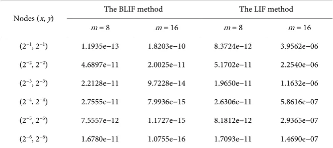
Table 4. The numerical results with Chebyshev nodes, M = 8, N = 7, example 1.

Nodes (x, y) The BLIF method The LIF method

m = 8 m = 16 m = 8 m = 16

(2−1_{, 2}−1_{) 1.1935e−13 1.8203e−10 8.3724e−12 3.9562e−06}

(2−2_{, 2}−2_{) 4.6897e−11 2.0025e−11 5.1702e−11 2.2540e−06}

(2−3_{, 2}−3_{) 2.2128e−11 9.7228e−14 1.9650e−11 1.1632e−06}

(2−4_{, 2}−4_{) 2.7555e−11 7.9936e−15 2.6306e−11 5.8616e−07}

(2−5_{, 2}−5_{) 7.5557e−12 1.1727e−15 8.1812e−12 2.9365e−07}

the numerical results of the BLIF method and the LIF method. We can conclude that the barycentric Lagrange method is more efficient and stable than the La-grange method.

Example 2. Consider two dimensional Fredholm integral equation of the fol-lowing form

(

) ( )

(

) (

)

[ ]

π ₁

2 ₂

0 0 ( ( , )

π

, d d , , , 0, 0,1 , 2

x y

e u x y

x y x y s t u s t t s f x y x y +

 

= + + + ⋅ + ∈_{ }×

 

∫ ∫

(15)

where

( ) (

)

(

)

(

)

π

3 2 2 2

π π

2 2 2

2 2

, 1 1

1

1 1 π 1 1 ,

2

x y

f x y e e x y x y

e e e x y e +

 

= − _ − _ +

 

  _{ }   

+ − _ _ − _− + −_{ }  _ +

    

 

the accurate solution is ( , ) x y

[image:6.595.207.540.422.551.2]

u x y =e + .

Table 5 and Table 6 reveal that the absolute and relative errors of the bary-centric and Lagrangian methods with m= =n 8,16 at the interior points. Gen-erally, the approximate solutions of barycentric method are more accurate than Lagrange method, especially for large node numbers. In the tables, the absolute errors are decreasing by barycentric method and increasing by the Lagrange method with the increasing of Chebyshev node numbers. In a word, the BLIF

Table 5. The absolute errors with Chebyshev nodes, M = N = 11, example 2.

Nodes (x, y) The BLIF method The LIF method

m = 8 m = 16 m = 8 m = 16

(0.1, 0.1) 2.2598e−09 6.6613e−16 2.2597e−09 2.4946e−08 (0.3, 0.3) 4.5070e−09 6.6613e−16 4.5078e−09 5.3816e−07 (0.5, 0.5) 1.3426e−09 1.3323e−15 1.3395e−09 1.9373e−06 (0.7, 0.7) 8.2825e−09 0.0000e−00 8.2724e−09 4.4205e−06 (0.9, 0.9) 1.2460e−08 1.7764e−15 1.2495e−08 1.7531e−05

Table 6. The absolute errors with Chebyshev nodes, M = N = 11, example 2.

Nodes (x, y) The BLIF method The LIF method

m = 8 m = 16 m = 8 m = 16

(2−1_{, 2}−1_{) 1.3426e−09 1.3323e−15 1.3395e−09 1.9373e−06}

(2−2_{, 2}−2_{) 1.4203e−09 1.1102e−15 1.4208e−09 3.3037e−07}

(2−3_{, 2}−3_{) 3.1271e−09 1.5543e−15 3.1270e−09 4.6671e−08}

(2−4_{, 2}−4_{) 1.7789e−10 1.5543e−15 1.7788e−10 6.3278e−09}

(2−5_{, 2}−5_{) 1.1286e−09 4.4409e−15 1.1287e−09 8.1572e−10}

[image:6.595.207.540.585.732.2]

method is more efficient than the LIF method which is agreement with the theoretical analysis.

5. Conclusion

In this paper, we solve two dimensional linear Fredholm integral equations of the second kind by means of the barycentric Lagrange interpolation method. The modified Lagrange method with Chebyshev nodes transforms the equations into linear algebraic equations, and the corresponding numerical solutions are stable forward. The numerical results also demonstrate that the barycentric me-thod is a simple and powerful technique. Furthermore, the barycentric meme-thod can extend to solve high dimensional FIEs.

Acknowledgements

The authors are very grateful to the reviewers. This work was partially supported by the financial support from National Natural Science Foundation of China (Grant no. 11371079).

References

[1] Yoshida, N., Imai, T., Phongphanphanee, S., Kovalenko, A. and Hirata, F. (2009) Molecular Recognition in Biomolecules Studied by Statistical-Mechanical Integral- Equation Theory of Liquids. Journal of Physical Chemistry B, 113, 873-886.

https://doi.org/10.1021/jp807068k

[2] Farengo, R., Lee, Y.C. and Guzdar, P.N. (1983) An Electromagnetic Integral Equa-tion: Application to Microtearing Modes. Physical Fluids, 26, 3515-3523.

https://doi.org/10.1063/1.864112

[3] Kosarev, E.L. (1980) Applications of Integral Equations of the First Kind in Experi-ment Physics. Computer Physics Communications, 20, 69-75.

https://doi.org/10.1016/0010-4655(80)90110-1

[4] Alipanah, A. and Esmaeili, S. (2011) Numerical Solution of the Two Dimensional Fredholm Integral Equations Using Gaussian Radial Basis Function. Journal of Com-putational and Applied Mathematics, 235, 5342-5347.

https://doi.org/10.1016/j.cam.2009.11.053

[5] Derili, H., Sohrabi, S. and Arzhang, A. (2012) Two-Dimensional Wavelets for Nu-merical Solution of Integral Equations. Mathematical Sciences, 6, 1-4.

[6] Heydari, M., Avazzadeh, Z., Navabpour, H. and Loghmani, G.B. (2013) Numerical Solution of Fredholm Integral Equations of the Second Kind by Using Integral Mean Value Theorem II. High Dimensional Problems. Applied Mathematical Modelling, 37, 432-442. https://doi.org/10.1016/j.apm.2012.03.011

[7] Ma, Y.Y., Huang, J. and Li, H. (2015) A Novel Numerical Method of Two-Dimen- sional Fredholm Integral Equations of the Second Kind. Mathematical Problems in Engineering, 2015, Article ID: 625013. https://doi.org/10.1155/2015/625013

[8] Berrut, J.-P. and Trefethen, L.N. (2004) Barycentric Lagrange Interpolation. SIAM Review, 46, 501-517. https://doi.org/10.1137/S0036144502417715

[9] Higham, N.J. (2004) The Numerical Stability of Barycentric Lagrange Interpolation,.

IMA Journal of Numerical Analysis, 24, 547-556.

https://doi.org/10.1093/imanum/24.4.547

Cheby-shev Points of the Second Kind. Numerische Mathematik, 128, 265-300.

https://doi.org/10.1007/s00211-014-0612-6

[11]Mascarenhas, W.F. and Camargo, A.P.D. (2014) On the Backward Stability of the Second Barycentric Formula for Interpolation. Dolomites Research Notes on Ap-proximation, 7, 1-13.

[12]Mustafa, M.M. and Muhammad, A.M. (2014) Numerical Solution of Linear Volter-ra-Fredholm Integro-Differential Equations Using Lagrange Polynomials. Mathe-matical Theory and Modeling, 4, 158-167.

[13]Lv, T. and Huang, J. (2013) A High Precision Algorithm for Integral Equation. Chi-na Science Publishing. (In Chinese)

Submit or recommend next manuscript to SCIRP and we will provide best service for you:

Accepting pre-submission inquiries through Email, Facebook, LinkedIn, Twitter, etc. A wide selection of journals (inclusive of 9 subjects, more than 200 journals)

Providing 24-hour high-quality service User-friendly online submission system Fair and swift peer-review system

Efficient typesetting and proofreading procedure

Display of the result of downloads and visits, as well as the number of cited articles Maximum dissemination of your research work

Submit your manuscript at: http://papersubmission.scirp.org/