Physics, Topology, Logic and Computation:
A Rosetta Stone
John C. Baez
Department of Mathematics, University of California Riverside, California 92521, USA
Mike Stay
Computer Science Department, University of Auckland and
Google, 1600 Amphitheatre Pkwy Mountain View, California 94043, USA email: [email protected], [email protected]
March 2, 2009
Abstract
In physics, Feynman diagrams are used to reason about quantum processes. In the 1980s, it became clear that underlying these diagrams is a powerful analogy between quantum physics and topology. Namely, a lin-ear operator behaves very much like a ‘cobordism’: a manifold representing spacetime, going between two manifolds representing space. This led to a burst of work on topological quantum field theory and ‘quan-tum topology’. But this was just the beginning: similar diagrams can be used to reason about logic, where they represent proofs, and computation, where they represent programs. With the rise of interest in quantum cryptography and quantum computation, it became clear that there is extensive network of analogies between physics, topology, logic and computation. In this expository paper, we make some of these analogies pre-cise using the concept of ‘closed symmetric monoidal category’. We assume no prior knowledge of category theory, proof theory or computer science.
1
Introduction
Category theory is a very general formalism, but there is a certain special way that physicists use categories which turns out to have close analogues in topology, logic and computation. A category hasobjectsand mor-phisms, which representthingsandways to go between things. In physics, the objects are oftenphysical systems, and the morphisms areprocessesturning a state of one physical system into a state of another system — per-haps the same one. In quantum physics we often formalize this by takingHilbert spacesas objects, andlinear operatorsas morphisms.
Sometime around 1949, Feynman [57] realized that in quantum field theory it is useful to draw linear oper-ators as diagrams:
This lets us reason with them pictorially. We can warp a picture without changing the operator it stands for: all that matters is the topology, not the geometry. In the 1970s, Penrose realized that generalizations of Feynman diagrams arise throughout quantum theory, and might even lead to revisions in our understanding of space-time [78]. In the 1980s, it became clear that underlying these diagrams is a powerful analogy between quan-tum physics and topology! Namely, a linear operator behaves very much like a ‘cobordism’ — that is, an n-dimensional manifold going between manifolds of one dimension less:
String theory exploits this analogy by replacing the Feynman diagrams of ordinary quantum field theory with 2-dimensional cobordisms, which represent the worldsheets traced out by strings with the passage of time. The analogy between operators and cobordisms is also important in loop quantum gravity and — most of all — the more purely mathematical discipline of ‘topological quantum field theory’.
Meanwhile, quite separately, logicians had begun using categories where the objects representpropositions and the morphisms representproofs. The idea is that a proof is a process going from one proposition (the hypothesis) to another (the conclusion). Later, computer scientists started using categories where the objects representdata typesand the morphisms representprograms. They also started using ‘flow charts’ to describe programs. Abstractly, these are very much like Feynman diagrams!
The logicians and computer scientists were never very far from each other. Indeed, the ‘Curry–Howard correspondence’ relating proofs to programs has been well-known at least since the early 1970s, with roots stretching back earlier [35, 52]. But, it is only in the 1990s that the logicians and computer scientists bumped into the physicists and topologists. One reason is the rise of interest in quantum cryptography and quantum computation [28]. With this, people began to think of quantum processes as forms of information processing, and apply ideas from computer science. It was then realized that the loose analogy between flow charts and Feynman diagrams could be made more precise and powerful with the aid of category theory [3].
By now there is an extensive network of interlocking analogies between physics, topology, logic and com-puter science. They suggest that research in the area of common overlap is actually trying to build a new science:
a general science of systems and processes. Building this science will be very difficult. There are good reasons for this, but also bad ones. One bad reason is that different fields use different terminology and notation.
The original Rosetta Stone, created in 196 BC, contains versions of the same text in three languages: de-motic Egyptian, hieroglyphic script and classical Greek. Its rediscovery by Napoleon’s soldiers let modern Egyptologists decipher the hieroglyphs. Eventually this led to a vast increase in our understanding of Egyptian culture.
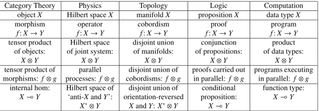
At present, the deductive systems in mathematical logic look like hieroglyphs to most physicists. Similarly, quantum field theory is Greek to most computer scientists, and so on. So, there is a need for a new Rosetta Stone to aid researchers attempting to translate between fields. Table 1 shows our guess as to what this Rosetta Stone might look like.
Category Theory Physics Topology Logic Computation object system manifold proposition data type morphism process cobordism proof program
Table 1: The Rosetta Stone (pocket version)
The rest of this paper expands on this table by comparing how categories are used in physics, topology, logic, and computation. Unfortunately, these different fields focus on slightly different kinds of categories. Though most physicists don’t know it, quantum physics has long made use of ‘compact symmetric monoidal categories’. Knot theory uses ‘compact braided monoidal categories’, which are slightly more general. However, it became clear in the 1990’s that these more general gadgets are useful in physics too. Logic and computer science used to focus on ‘cartesian closed categories’ — where ‘cartesian’ can be seen, roughly, as an antonym of ‘quantum’. However, thanks to work on linear logic and quantum computation, some logicians and computer scientists have dropped their insistence on cartesianness: now they study more general sorts of ‘closed symmetric monoidal categories’.
In Section 2 we explain these concepts, how they illuminate the analogy between physics and topology, and how to work with them using string diagrams. We assume no prior knowledge of category theory, only a willingness to learn some. In Section 3 we explain how closed symmetric monoidal categories correspond to a small fragment of ordinary propositional logic, which also happens to be a fragment of Girard’s ‘linear logic’ [43]. In Section 4 we explain how closed symmetric monoidal categories correspond to a simple model of computation. Each of these sections starts with some background material. In Section 5, we conclude by presenting a larger version of the Rosetta Stone.
Our treatment of all four subjects — physics, topology, logic and computation — is bound to seem sketchy, narrowly focused and idiosyncratic to practitioners of these subjects. Our excuse is that we wish to empha-size certain analogies while saying no more than absolutely necessary. To make up for this, we include many references for those who wish to dig deeper.
2
The Analogy Between Physics and Topology
2.1
Background
Currently our best theories of physics are general relativity and the Standard Model of particle physics. The first describes gravity without taking quantum theory into account; the second describes all the other forces taking quantum theory into account, but ignores gravity. So, our world-view is deeply schizophrenic. The field where physicists struggle to solve this problem is calledquantum gravity, since it is widely believed that the solution requires treating gravity in a way that takes quantum theory into account.
Physics Topology
Hilbert space (n−1)-dimensional manifold
(system) (space)
operator between cobordism between Hilbert spaces (n−1)-dimensional manifolds
(process) (spacetime) composition of operators composition of cobordisms
identity operator identity cobordism Table 2: Analogy between physics and topology
Nobody is sure how to do this, but there is a striking similarity between two of the main approaches: string theory and loop quantum gravity. Both rely on the analogy between physics and topology shown in Table 2. On the left we have a basic ingredient of quantum theory: the category Hilb whose objects are Hilbert spaces, used to describe physicalsystems, and whose morphisms are linear operators, used to describe physicalprocesses. On the right we have a basic structure in differential topology: the categorynCob. Here the objects are (n− 1)-dimensional manifolds, used to describespace, and whose morphisms aren-dimensional cobordisms, used to describespacetime.
As we shall see, Hilb and nCob share many structural features. Moreover, both are very different from the more familiar category Set, whose objects are sets and whose morphisms are functions. Elsewhere we have argued at great length that this is important for better understanding quantum gravity [10] and even the foundations of quantum theory [11]. The idea is that if Hilb is more likenCob than Set, maybe we should stop thinking of a quantum process as a function from one set of states to another. Instead, maybe we should think of it as resembling a ‘spacetime’ going between spaces of dimension one less.
This idea sounds strange, but the simplest example is something very practical, used by physicists every day: a Feynman diagram. This is a 1-dimensional graph going between 0-dimensional collections of points, with edges and vertices labelled in certain ways. Feynman diagrams are topological entities, but they describe linear operators. String theory uses 2-dimensional cobordisms equipped with extra structure — string worldsheets — to do a similar job. Loop quantum gravity uses 2d generalizations of Feynman diagrams called ‘spin foams’ [9]. Topological quantum field theory uses higher-dimensional cobordisms [13]. In each case, processes are described by morphisms in a special sort of category: a ‘compact symmetric monoidal category’.
In what follows, we shall not dwell on puzzles from quantum theory or quantum gravity. Instead we take a different tack, simply explaining some basic concepts from category theory and showing how Set, Hilb,nCob
and categories of tangles give examples. A recurring theme, however, is that Set is very different from the other examples.
To help the reader safely navigate the sea of jargon, here is a chart of the concepts we shall explain in this section: categories monoidal categories R R R R R R R R R R R R R R braided monoidal categories Q Q Q Q Q Q Q Q Q Q Q Q Q closed monoidal categories Q Q Q Q Q Q Q Q Q Q Q Q Q symmetric monoidal categories Q Q Q Q Q Q Q Q Q Q Q Q closed braided monoidal categories Q Q Q Q Q Q Q Q Q Q Q Q Q compact monoidal categories
cartesian categories closed symmetric monoidal categories mmmmmm mmmmmm m Q Q Q Q Q Q Q Q Q Q Q Q compact braided monoidal categories cartesian closed categories compact symmetric monoidal categories
The category Set is cartesian closed, while Hilb andnCob are compact symmetric monoidal.
2.2
Categories
Category theory was born around 1945, with Eilenberg and Mac Lane [40] defining ‘categories’, ‘functors’ between categories, and ‘natural transformations’ between functors. By now there are many introductions to the subject [34, 72, 75], including some available for free online [20, 46]. Nonetheless, we begin at the beginning:
Definition 1 AcategoryC consists of:
• a collection ofobjects, where if X is an object of C we write X∈C, and
• for every pair of objects(X,Y),a sethom(X,Y)ofmorphismsfrom X to Y. We call this sethom(X,Y)a
homset. If f ∈hom(X,Y),then we write f:X→Y.
such that:
• morphisms are composable: given f:X→Y and g:Y →Z,there is acomposite morphismg f:X→Z; sometimes also written g◦ f .
• an identity morphism is both aleft and a right unitfor composition: if f:X→ Y,then f1X = f =1Yf; and
• composition isassociative:(hg)f =h(g f)whenever either side is well-defined.
Definition 2 We say a morphism f:X→Y is anisomorphismif it has an inverse— that is, there exists another morphism g:Y →X such that g f =1Xand f g=1Y.
A category is the simplest framework where we can talk about systems (objects) and processes (morphisms). To visualize these, we can use ‘Feynman diagrams’ of a very primitive sort. In applications to linear algebra, these diagrams are often called ‘spin networks’, but category theorists call them ‘string diagrams’, and that is the term we will use. The term ‘string’ here has little to do with string theory: instead, the idea is that objects of our category label ‘strings’ or ‘wires’:
X
and morphismsf:X→Y label ‘black boxes’ with an input wire of typeXand an output wire of typeY:
f X
Y
We compose two morphisms by connecting the output of one black box to the input of the next. So, the composite off:X→Yandg:Y→Zlooks like this:
f
g X
Y
Z
f
g
h X
Y
Z
W
is our notation for bothh(g f) and (hg)f. Similarly, if we draw the identity morphism 1X:X →Xas a piece of wire of typeX:
X
then the left and right unit laws are also implicit.
There are countless examples of categories, but we will focus on four:
• Set: the category where objects are sets.
• Hilb: the category where objects are finite-dimensional Hilbert spaces.
• nCob: the category where morphisms aren-dimensional cobordisms.
• Tangk: the category where morphisms arek-codimensional tangles.
As we shall see, all four are closed symmetric monoidal categories, at least whenkis big enough. However, the most familiar of the lot, namely Set, is the odd man out: it is ‘cartesian’.
Traditionally, mathematics has been founded on the category Set, where the objects aresetsand the mor-phisms arefunctions. So, when we study systems and processes in physics, it is tempting to specify a system by giving its set of states, and a process by giving a function from states of one system to states of another.
However, in quantum physics we do something subtly different: we use categories where objects areHilbert spacesand morphisms arebounded linear operators. We specify a system by giving a Hilbert space, but this Hilbert space is not really the set of states of the system: a state is actually a ray in Hilbert space. Similarly, a bounded linear operator is not precisely a function from states of one system to states of another.
In the day-to-day practice of quantum physics, what really matters is not sets of states and functions between them, but Hilbert space and operators. One of the virtues of category theory is that it frees us from the ‘Set-centric’ view of traditional mathematics and lets us view quantum physics on its own terms. As we shall see, this sheds new light on the quandaries that have always plagued our understanding of the quantum realm [11].
To avoid technical issues that would take us far afield, we will take Hilb to be the category where objects arefinite-dimensional Hilbert spacesand morphisms arelinear operators(automatically bounded in this case). Finite-dimensional Hilbert spaces suffice for some purposes; infinite-dimensional ones are often important, but treating them correctly would require some significant extensions of the ideas we want to explain here.
In physics we also use categories where the objects represent choices ofspace, and the morphisms represent choices ofspacetime. The simplest is nCob, where the objects are (n−1)-dimensional manifolds, and the morphisms aren-dimensional cobordisms. Glossing over some subtleties that a careful treatment would discuss [81], a cobordism f:X →Yis ann-dimensional manifold whose boundary is the disjoint union of the (n− 1)-dimensional manifoldsXandY. Here are a couple of cobordisms in the casen=2:
X
Y f
Y
Z g
We compose them by gluing the ‘output’ of one to the ‘input’ of the other. So, in the above exampleg f:X→Z looks like this:
X
Z g f
Another kind of category important in physics has objects representingcollections of particles, and mor-phisms representing theirworldlines and interactions. Feynman diagrams are the classic example, but in these diagrams the ‘edges’ are not taken literally as particle trajectories. An example with closer ties to topology is Tangk.
Very roughly speaking, an object in Tangkis a collection of points in ak-dimensional cube, while a morphism is a ‘tangle’: a collection of arcs and circles smoothly embedded in a (k+1)-dimensional cube, such that the circles lie in the interior of the cube, while the arcs touch the boundary of the cube only at its top and bottom, and only at their endpoints. A bit more precisely, tangles are ‘isotopy classes’ of such embedded arcs and circles: this equivalence relation means that only the topology of the tangle matters, not its geometry. We compose tangles by attaching one cube to another top to bottom.
More precise definitions can be found in many sources, at least fork = 2, which gives tangles in a 3-dimensional cube [42, 58, 81, 89, 97, 101]. But since a picture is worth a thousand words, here is a picture of a
morphism in Tang2:
X
Y f
Note that we can think of a morphism in Tangkas a 1-dimensional cobordismembedded in a k-dimensional cube. This is why TangkandnCob behave similarly in some respects.
Here are two composable morphisms in Tang1: X
Y f
Y
Z g
and here is their composite:
X
Z g f
Since only the tangle’s topology matters, we are free to squash this rectangle into a square if we want, but we do not need to.
It is often useful to consider tangles that are decorated in various ways. For example, in an ‘oriented’ tangle, each arc and circle is equipped with an orientation. We can indicate this by drawing a little arrow on each curve in the tangle. In applications to physics, these curves represent worldlines of particles, and the arrows
say whether each particle is going forwards or backwards in time, following Feynman’s idea that antiparticles are particles going backwards in time. We can also consider ‘framed’ tangles. Here each curve is replaced by a ‘ribbon’. In applications to physics, this keeps track of how each particle twists. This is especially important for fermions, where a 2πtwist acts nontrivially. Mathematically, the best-behaved tangles are both framed and oriented [13, 89], and these are what we should use to define Tangk. The categorynCob also has a framed oriented version. However, these details will barely matter in what is to come.
It is difficult to do much with categories without discussing the maps between them. A map between cate-gories is called a ‘functor’:
Definition 3 AfunctorF:C→D from a category C to a category D is a map sending:
• any object X∈C to an object F(X)∈D,
• any morphism f:X→Y in C to a morphism F(f):F(X)→F(Y)in D, in such a way that:
• Fpreserves identities: for any object X∈C, F(1X)=1F(X);
• Fpreserves composition: for any pair of morphisms f:X→Y, g:Y→Z in C, F(g f)=F(g)F(f). In the sections to come, we will see that functors and natural transformations are useful for putting extra structure on categories. Here is a rather different use for functors: we can think of a functorF:C→Das giving a picture, or ‘representation’, ofCinD. The idea is thatFcan map objects and morphisms of some ‘abstract’ categoryCto objects and morphisms of a more ‘concrete’ categoryD.
For example, consider an abstract groupG. This is the same as a category with one object and with all morphisms invertible. The object is uninteresting, so we can just call it•, but the morphisms are the elements ofG, and we compose them by multiplying them. From this perspective, arepresentationofGon a finite-dimensional Hilbert space is the same as a functorF:G→Hilb. Similarly, anactionofGon a set is the same as a functorF:G→Set. Both notions are ways of making an abstract group more concrete.
Ever since Lawvere’s 1963 thesis on functorial semantics [69], the idea of functors as representations has become pervasive. However, the terminology varies from field to field. Following Lawvere, logicians often call the categoryCa ‘theory’, and call the functorF:C→Da ‘model’ of this theory. Other mathematicians might callFan ‘algebra’ of the theory. In this work, the default choice ofDis usually the category Set.
In physics, it is the functorF:C → Dthat is called the ‘theory’. Here the default choice ofDis either the category we are calling Hilb or a similar category ofinfinite-dimensionalHilbert spaces. For example, both ‘conformal field theories’ [85] and topological quantum field theories [8] can be seen as functors of this sort.
If we think of functors as models, natural transformations are maps between models:
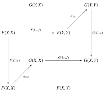
Definition 4 Given two functors F,F0:C→D,anatural transformationα:F⇒F0assigns to every object X in C a morphismαX:F(X)→F0(X)such that for any morphism f:X→Y in C,the equationαYF(f)=F0(f)αX
holds in D.In other words, this square commutes:
F(X) F(Y)
F0(X) F0(Y)
-F(f)
? αX
? αY
-F0(f)
(Going across and then down equals going down and then across.)
Definition 5 Anatural isomorphismbetween functors F,F0:C → D is a natural transformationα:F ⇒ F0 such thatαXis an isomorphism for every X∈C.
For example, supposeF,F0:G → Hilb are functors whereGis a group, thought of as a category with one object, say•. Then, as already mentioned,FandF0are secretly just representations ofGon the Hilbert spaces F(•) andF0(•). A natural transformationα:F ⇒ F0is then the same as anintertwining operatorfrom one representation to another: that is, a linear operator
A:F(•)→F0(•) satisfying
AF(g)=F0(g)A for all group elementsg.
2.3
Monoidal Categories
In physics, it is often useful to think of two systems sitting side by side as forming a single system. In topology, the disjoint union of two manifolds is again a manifold in its own right. In logic, the conjunction of two statement is again a statement. In programming we can combine two data types into a single ‘product type’. The concept of ‘monoidal category’ unifies all these examples in a single framework.
A monoidal categoryChas a functor⊗:C×C →Cthat takes two objectsXandYand puts them together to give a new objectX⊗Y. To make this precise, we need the cartesian product of categories:
Definition 6 Thecartesian productC×C0of categories C and C0is the category where:
• an object is a pair(X,X0)consisting of an object X∈C and an object X0∈C0;
• a morphism from(X,X0)to(Y,Y0)is a pair(f,f0)consisting of a morphism f:X → Y and a morphism f0:X0→Y0;
• composition is done componentwise:(g,g0)(f,f0)=(g f,g0f0);
Mac Lane [71] defined monoidal categories in 1963. The subtlety of the definition lies in the fact that (X⊗Y)⊗ZandX⊗(Y⊗Z) are not usually equal. Instead, we should specify an isomorphism between them, called the ‘associator’. Similarly, while a monoidal category has a ‘unit object’I, it is not usually true thatI⊗X andX⊗IequalX. Instead, we should specify isomorphismsI⊗XXandX⊗I X. To be manageable, all these isomorphisms must then satisfy certain equations:
Definition 7 Amonoidal categoryconsists of:
• a category C,
• atensor productfunctor⊗:C×C→C,
• aunit objectI∈C,
• a natural isomorphism called theassociator, assigning to each triple of objects X,Y,Z ∈C an isomor-phism
aX,Y,Z: (X⊗Y)⊗Z→∼ X⊗(Y⊗Z),
• natural isomorphisms called theleftandright unitors, assigning to each object X∈C isomorphisms lX:I⊗X
∼
→X
rX :X⊗I
∼
→X,
such that:
• for all X,Y∈C thetriangle equationholds:
(X⊗I)⊗Y X⊗(I⊗Y)
X⊗Y
-aX,I,Y
Q Q
QQs
rX⊗1Y
• for all W,X,Y,Z∈C, thepentagon equationholds:
((W⊗X)⊗Y)⊗Z
(W⊗(X⊗Y))⊗Z
(W⊗X)⊗(Y⊗Z)
W⊗((X⊗Y)⊗Z)
W⊗(X⊗(Y⊗Z)) aW⊗X,Y,Z
HH HH
HHHj
aW,X,Y⊗1Z
?
aW,X⊗Y,Z @ @ @ @ @ @ @ @ R
aW,X,Y⊗Z
1W⊗aX,Y,Z
When we have a tensor product of four objects, there are five ways to parenthesize it, and at first glance the associator lets us build two isomorphisms fromW⊗(X⊗(Y⊗Z)) to ((W⊗X)⊗Y)⊗Z. But, the pentagon equation says these isomorphisms are equal. When we have tensor products of even more objects there are even more ways to parenthesize them, and even more isomorphisms between them built from the associator. However, Mac Lane showed that the pentagon identity implies these isomorphisms are all the same. Similarly, if we also assume the triangle equation, all isomorphisms with the same source and target built from the associator, left and right unit laws are equal.
In a monoidal category we can do processes in ‘parallel’ as well as in ‘series’. Doing processes in series is just composition of morphisms, which works in any category. But in a monoidal category we can also tensor morphismsf:X→Yandf0:X0→Y0and obtain a ‘parallel process’ f⊗f0:X⊗X0→Y⊗Y0. We can draw this in various ways:
f X Y f0 X0 Y0
= f⊗f0
X
Y
X0
Y0
= f ⊗f0 X⊗X0
Y⊗Y0
More generally, we can draw any morphism
as a black box withninput wires andmoutput wires:
f
X1 X2 X3
Y1 Y2
We draw the unit objectIas a blank space. So, for example, we draw a morphismf:I→Xas follows:
f X
By composing and tensoring morphisms, we can build up elaborate pictures resembling Feynman diagrams:
f g
h
j
X1 X2 X3 X4
Y1 Y2 Y3 Y4
Z
The laws governing a monoidal category allow us to neglect associators and unitors when drawing such pictures, without getting in trouble. The reason is that Mac Lane’s Coherence Theorem says any monoidal category is ‘equivalent’, in a suitable sense, to one where all associators and unitors are identity morphisms [71].
We can also deform the picture in a wide variety of ways without changing the morphism it describes. For example, the above morphism equals this one:
f
g
h
j
X1 X2 X3 X4
Everyone who uses string diagrams for calculations in monoidal categories starts by worrying about the rules of the game:precisely howcan we deform these pictures without changing the morphisms they describe? Instead of stating the rules precisely — which gets a bit technical — we urge you to explore for yourself what is allowed and what is not. For example, show that we can slide black boxes up and down like this:
f g X1
Y1
X2
Y2
= f g
X1
Y1
X2
Y2
=
f g X1
Y1
X2
Y2
For a formal treatment of the rules governing string diagrams, try the original papers by Joyal and Street [55] and the book by Yetter [101].
Now let us turn to examples. Here it is crucial to realize that the same category can often be equipped with different tensor products, resulting in different monoidal categories:
• There is a way to make Set into a monoidal category where X⊗Y is the cartesian productX×Y and the unit object is any one-element set. Note that this tensor product is not strictly associative, since (x,(y,z)) , ((x,y),z),but there’s a natural isomorphism (X ×Y)×Z X ×(Y ×Z), and this is our associator. Similar considerations give the left and right unitors. In this monoidal category, the tensor product of f:X→Yand f0:X0→Y0is the function
f ×f0 :X×X0 → Y×Y0 (x,x0) 7→ (f(x),f0(x0)).
There is also a way to make Set into a monoidal category whereX⊗Y is the disjoint union ofX and Y, which we shall denote byX+Y. Here the unit object is the empty set. Again, as indeed with all these examples, the associative law and left/right unit laws hold only up to natural isomorphism. In this monoidal category, the tensor product of f:X→Yand f0:X0→Y0is the function
f+f0: X+X0 → Y+Y0
x 7→
(
f(x) ifx∈X, f0(x) ifx∈X0.
However, in what follows, when we speak of Setas a monoidal category, we always use the cartesian product!
• There is a way to make Hilb into a monoidal category with the usual tensor product of Hilbert spaces:
Cn⊗CmCnm.In this case the unit objectIcan be taken to be a 1-dimensional Hilbert space, for example
C.
There is also a way to make Hilb into a monoidal category where the tensor product is the direct sum:
Cn⊕CmCn+m.In this case the unit object is the zero-dimensional Hilbert space,{0}.
However, in what follows, when we speak ofHilbas a monoidal category, we always use the usual tensor product!
• The tensor product of objects and morphisms innCob is given by disjoint union. For example, the tensor product of these two morphisms:
X
Y f
X0
Y0 f0
is this:
X⊗X0
Y⊗Y0 f⊗f0
• The category Tangkis monoidal whenk≥1, where the the tensor product is given by disjoint union. For example, given these two tangles:
X
Y f
X0
Y0 f0
their tensor product looks like this:
X⊗X0
Y⊗Y0 f⊗f0
The example of Set with its cartesian product is different from our other three main examples, because the cartesian product of setsX×X0comes equipped with functions called ‘projections’ to the setsXandX0:
X p X×X0 p- X0
Our other main examples lack this feature — though Hilb made into a monoidal category using⊕has projections. Also, every set has a unique function to the one-element set:
!X:X→I.
Again, our other main examples lack this feature, though Hilb made into a monoidal category using⊕has it. A fascinating feature of quantum mechanics is that we make Hilb into a monoidal category using⊗instead of⊕, even though the latter approach would lead to a category more like Set.
We can isolate the special features of the cartesian product of sets and its projections, obtaining a definition that applies to any category:
Definition 8 Given objects X and X0in some category, we say an object X×X0equipped with morphisms
X p X×X0 p- X0
0
is acartesian product(or simplyproduct) of X and X0if for any object Q and morphisms Q
X X0
f
@@Rf
0
there exists a unique morphism g:Q→X×X0making the following diagram commute: Q
X X×X0 X0
f @@
@ @ R
f0
?
g
p p0
-(That is, f =pg and f0=p0g.) We say a category hasbinary productsif every pair of objects has a product. The product may not exist, and it may not be unique, but when it exists it is unique up to a canonical iso-morphism. This justifies our speaking of ‘the’ product of objectsX andY when it exists, and denoting it as X×Y.
The definition of cartesian product, while absolutely fundamental, is a bit scary at first sight. To illustrate its power, let us do something with it: combine two morphisms f:X→Yandf0:X0→Y0into a single morphism
f ×f0:X×X0→Y×Y0.
The definition of cartesian product says how to build a morphism of this sort out of a pair of morphisms: namely, morphisms fromX×X0toYandY0. If we take these to be f pand f0p0, we obtain f×f0:
X×X0
Y Y×Y0 Y0
f p @@
@ @ R
f0p0
?
f×f0
p p0
Definition 9 An object1in a category C isterminalif for any object Q∈C there exists a unique morphism from Q to1, which we denote as!Q:Q→1.
Again, a terminal object may not exist and may not be unique, but it is unique up to a canonical isomorphism. This is why we can speak of ‘the’ terminal object of a category, and denote it by a specific symbol, 1.
We have introduced the concept of binary products. One can also talk aboutn-ary products for other values ofn, but a category with binary products hasn-ary products for alln≥1, since we can construct these as iterated binary products. The casen=1 is trivial, since the product of one object is just that object itself (up to canonical isomorphism). The remaining case isn =0. The zero-ary product of objects, if it exists, is just the terminal object. So, we make the following definition:
Definition 10 A category hasfinite productsif it has binary products and a terminal object.
A category with finite products can always be made into a monoidal category by choosing a specific product X×Yto be the tensor productX⊗Y, and choosing a specific terminal object to be the unit object. It takes a bit of work to show this! A monoidal category of this form is calledcartesian.
In a cartesian category, we can ‘duplicate and delete information’. In general, the definition of cartesian products gives a way to take two morphisms f1:Q → X and f2:Q → Y and combine them into a single
morphism fromQtoX×Y. If we takeQ=X=Yand take f1and f2to be the identity, we obtain thediagonal
orduplicationmorphism:
∆X:X→X×X.
In the category Set one can check that this maps any elementx∈ Xto the pair (x,x). In general, we can draw the diagonal as follows:
∆ X
X X
Similarly, we call the unique map to the terminal object !X:X→1 thedeletionmorphism, and draw it as follows:
! X
A fundamental fact about cartesian categories is that duplicating something and then deleting either copy is the same as doing nothing at all! In string diagrams, this says:
! ∆ X
X
X =
X
=
! ∆ X
X X
We leave the proof as an exercise for the reader.
Many of the puzzling features of quantum theory come from the noncartesianness of the usual tensor product in Hilb. For example, in a cartesian category, every morphism
g
X X0
is actually of the form
f X
f0 X0
In the case of Set, this says that every point of the setX×X0comes from a point ofXand a point ofX0. In physics, this would say that every stategof the combined systemX⊗X0is built by combining states of the systemsXandX0. Bell’s theorem [19] says that isnottrue in quantum theory. The reason is that quantum theory uses the noncartesian monoidal category Hilb!
Also, in quantum theory wecannotfreely duplicate or delete information. Wootters and Zurek [100] proved a precise theorem to this effect, focused on duplication: the cloning theorem’. One can also prove a ‘no-deletion theorem’. Again, these results rely on the noncartesian tensor product in Hilb.
2.4
Braided Monoidal Categories
In physics, there is often a process that lets us ‘switch’ two systems by moving them around each other. In topology, there is a tangle that describes the process of switching two points:
In logic, we can switch the order of two statements in a conjunction: the statement ‘XandY’ is isomorphic to ‘YandX’. In computation, there is a simple program that switches the order of two pieces of data. A monoidal category in which we can do this sort of thing is called ‘braided’:
Definition 11 Abraided monoidal categoryconsists of:
• a monoidal category C,
• a natural isomorphism called thebraidingthat assigns to every pair of objects X,Y∈C an isomorphism bX,Y:X⊗Y →Y⊗X,
such that thehexagon equationshold:
X⊗(Y⊗Z) (X⊗Y)⊗Z (Y⊗X)⊗Z
(Y⊗Z)⊗X Y⊗(Z⊗X) Y⊗(X⊗Z)
(X⊗Y)⊗Z X⊗(Y⊗Z) X⊗(Z⊗Y)
Z⊗(X⊗Y) (Z⊗X)⊗Y (X⊗Z)⊗Y
-a−1X,Y,Z
?
bX,Y⊗Z
-bX,Y⊗1Z
?
aY,X,Z
a−1
Y,Z,X
1Y⊗bX,Z
-aX,Y,Z
?
bX⊗Y,Z
-1X⊗bY,Z
?
a−1
X,Z,Y
aZ,X,Y
bX,Z⊗1Y
The first hexagon equation says that switching the objectXpastY⊗Zall at once is the same as switching it past Yand then pastZ(with some associators thrown in to move the parentheses). The second one is similar: it says switchingX⊗YpastZall at once is the same as doing it in two steps.
In string diagrams, we draw the braidingbX,Y:X⊗Y→Y⊗Xlike this:
We draw its inverseb−1
X,Ylike this:
X Y
This is a nice notation, because it makes the equations saying thatbX,Yandb−X1,Yare inverses ‘topologically true’:
X
X
Y
Y
= X Y =
Y
Y X
X Here are the hexagon equations as string diagrams:
X
X Y⊗Z
Y⊗Z
=
X Y Z
Y Z X
X⊗Y
X⊗Y Z
Z
=
Y Z
X
Y X Z
For practice, we urge you to prove the following equations:
f g
X
X0 Y
Y0
=
g f
X
X0 Y
Y0
Z
X Y
X Y
Z
=
Y Z
X
X Y
Z
If you get stuck, here are some hints. The first equation follows from the naturality of the braiding. The second is called theYang–Baxter equationand follows from a combination of naturality and the hexagon equations [56].
Next, here are some examples. There can be many different ways to give a monoidal category a braiding, or none. However, most of our favorite examples come with well-known ‘standard’ braidings:
• Any cartesian category automatically becomes braided, and in Set with its cartesian product, this standard braiding is given by:
bX,Y :X×Y → Y×X
(x,y) 7→ (y,x).
• In Hilb with its usual tensor product, the standard braiding is given by:
bX,Y :X⊗Y → Y⊗X
x⊗y 7→ y⊗x.
cylindersX×[0,1] andY×[0,1]. For 2Cob this braiding looks as follows whenXandYare circles: X⊗Y
Y⊗X
bX,Y
• The monoidal category Tangkhas a standard braiding whenk≥2. Fork=2 this looks as follows when XandY are each a single point:
X⊗Y
Y⊗X
bX,Y
The example of Tangkillustrates an important pattern. Tang0 is just a category, because in 0-dimensional space we can only do processes in ‘series’: that is, compose morphisms. Tang1is a monoidal category, because in 1-dimensional space we can also do processes in ‘parallel’: that is, tensor morphisms. Tang2 is a braided monoidal category, because in 2-dimensional space there is room to move one object around another. Next we shall see what happens when space has 3 or more dimensions!
2.5
Symmetric Monoidal Categories
Sometimes switching two objects and switching them again is the same as doing nothing at all. Indeed, this situation is very familiar. So, the first braided monoidal categories to be discovered were ‘symmetric’ ones [71]:
Definition 12 Asymmetric monoidal categoryis a braided monoidal category where the braiding satisfies bX,Y=b−Y,1X.
So, in a symmetric monoidal category,
X Y
Y X
or equivalently:
X Y
=
Y X
Any cartesian category automatically becomes a symmetric monoidal category, so Set is symmetric. It is also easy to check that Hilb,nCob are symmetric monoidal categories. So is Tangkfork≥3.
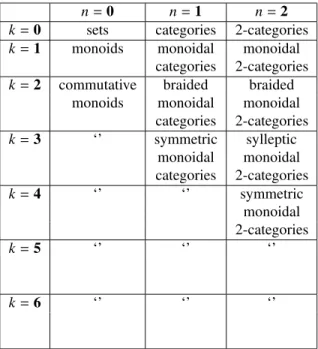
Interestingly, Tangk‘stabilizes’ atk=3: increasing the value ofkbeyond this value merely gives a category equivalent to Tang3. The reason is that we can already untie all knots in 4-dimensional space; adding extra dimensions has no real effect. In fact, Tangkfork≥3 is equivalent to 1Cob. This is part of a conjectured larger pattern called the ‘Periodic Table’ ofn-categories [13]. A piece of this is shown in Table 3.
Ann-category has not only morphisms going between objects, but 2-morphisms going between morphisms, 3-morphisms going between 2-morphisms and so on up ton-morphisms. In topology we can usen-categories to describe tangled higher-dimensional surfaces [14], and in physics we can use them to describe not just particles but also strings and higher-dimensional membranes [13, 15]. The Rosetta Stone we are describing concerns only then=1 column of the Periodic Table. So, it is probably just a fragment of a larger, still buriedn-categorical Rosetta Stone.
n=0 n=1 n=2
k=0 sets categories 2-categories k=1 monoids monoidal monoidal
categories 2-categories k=2 commutative braided braided
monoids monoidal monoidal categories 2-categories k=3 ‘’ symmetric sylleptic
monoidal monoidal categories 2-categories k=4 ‘’ ‘’ symmetric
monoidal 2-categories
k=5 ‘’ ‘’ ‘’
k=6 ‘’ ‘’ ‘’
2.6
Closed Categories
In quantum mechanics, one can encode a linear operatorf:X→Yinto a quantum state using a technique called ‘gate teleportation’ [47]. In topology, there is a way to take any tangle f:X→Yand bend the input back around to make it part of the output. In logic, we can take a proof that goes from some assumptionXto some conclusion Yand turn it into a proof that goes from no assumptions to the conclusion ‘XimpliesY’. In computer science, we can take any program that takes input of typeXand produces output of typeY, and think of it as a piece of data of a new type: a ‘function type’. The underlying concept that unifies all these examples is the concept of a ‘closed category’.
Given objectsXandYin any categoryC, there is asetof morphisms fromXtoY, denoted hom(X,Y). In a closed category there is also anobjectof morphisms fromXtoY, which we denote byX( Y. (Many other notations are also used.) In this situation we speak of an ‘internal hom’, since the objectX (Ylives insideC, instead of ‘outside’, in the category of sets.
Closed categories were introduced in 1966, by Eilenberg and Kelly [39]. While these authors were able to define a closed structure for any category, it turns out that the internal hom is most easily understood for monoidal categories. The reason is that when our category has a tensor product, it is closed precisely when morphisms fromX⊗Y toZare in natural one-to-one correspondence with morphisms fromY toX ( Z. In other words, it is closed when we have a natural isomorphism
hom(X⊗Y,Z) hom(Y,X(Z)
f 7→ f˜
For example, in the category Set, if we takeX⊗Y to be the cartesian productX×Y, thenX(Zis just the set of functions fromXtoZ, and we have a one-to-one correspondence between
• functions f that eat elements ofX×Y and spit out elements ofZ and
• functions ˜f that eat elements ofYand spit out functions fromXtoZ. This correspondence goes as follows:
˜
f(x)(y)=f(x,y).
Before considering other examples, we should make the definition of ‘closed monoidal category’ completely precise. For this we must note that for any categoryC, there is a functor
hom:Cop×C→Set.
Definition 13 Theopposite categoryCopof a category C has the same objects as C, but a morphism f:x→y in Copis a morphism f:y→x in C, and the composite g f in Copis the composite f g in C.
Definition 14 For any category C, thehom functor
sends any object(X,Y)∈Cop×C to the sethom(X,Y), and sends any morphism(f,g)∈Cop×C to the function
hom(f,g): hom(X,Y) → hom(X0,Y0)
h 7→ gh f
when f:X0→X and g:Y→Y0are morphisms in C.
Definition 15 A monoidal category C isleft closedif there is aninternal homfunctor (:Cop×C→C
together with a natural isomorphism c calledcurryingthat assigns to any objects X,Y,Z∈C a bijection cX,Y,Z: hom(X⊗Y,Z) →∼ hom(X,Y (Z)
It isright closedif there is an internal hom functor as above and a natural isomorphism cX,Y,Z: hom(X⊗Y,Z) →∼ hom(Y,X(Z).
The term ‘currying’ is mainly used in computer science, after the work of Curry [35]. In the rest of this section we only considerrightclosed monoidal categories. Luckily, there is no real difference between left and right closed for a braided monoidal category, as the braiding gives an isomorphismX⊗YY⊗X.
All our examples of monoidal categories are closed, but we shall see that, yet again, Set is different from the rest:
• The cartesian category Set is closed, whereX (Yis just the set of functions fromXtoY. In Set or any other cartesian closed category, the internal homX(Yis usually denotedYX. To minimize the number of different notations and emphasize analogies between different contexts, we shall not do this: we shall always useX(Y. To treat Set asleftclosed, we define the curried version off:X×Y→Zas above:
˜
f(x)(y)= f(x,y).
To treat it asrightclosed, we instead define it by ˜
f(y)(x)= f(x,y).
This looks a bit awkward, but it will be nice for string diagrams.
• The symmetric monoidal category Hilb with its usual tensor product is closed, whereX ( Y is the set of linear operators fromX toY, made into a Hilbert space in a standard way. In this case we have an isomorphism
X(Y X∗⊗Y
whereX∗ is the dual of the Hilbert spaceX, that is, the set of linear operators f:X → C, made into a Hilbert space in the usual way.
• The monoidal category Tangk(k≥1) is closed. As with Hilb, we have
X(Y X∗⊗Y
• The symmetric monoidal categorynCob is also closed; again
X(Y X∗⊗Y
whereX∗is the (n−1)-manifoldXwith its orientation reversed.
Except for Set, all these examples are actually ‘compact’. This basically means thatX(Yis isomorphic to X∗⊗Y, whereX∗is some object called the ‘dual’ ofX. But to make this precise, we need to define the ‘dual’ of an object in an arbitrary monoidal category.
To do this, let us generalize from the case of Hilb. As already mentioned, each objectX ∈Hilb has a dual X∗consisting of all linear operators f:X→I, where the unit objectIis justC. There is thus a linear operator
eX: X⊗X∗ → I
x⊗f 7→ f(x)
called thecounitofX. Furthermore, the space of all linear operators fromXtoY ∈Hilb can be identified with X∗⊗Y. So, there is also a linear operator called theunitofX:
iX: I → X∗⊗X
c 7→ c1X
sending any complex numbercto the corresponding multiple of the identity operator.
The significance of the unit and counit become clearer if we borrow some ideas from Feynman. In physics, if Xis the Hilbert space of internal states of some particle,X∗is the Hilbert space for the corresponding antiparticle. Feynman realized that it is enlightening to think of antiparticles as particles going backwards in time. So, we draw a wire labelled byX∗as a wire labelled byX, but with an arrow pointing ‘backwards in time’: that is, up instead of down:
X∗ = X
(Here we should admit that most physicists use the opposite convention, where time marches up the page. Since we read from top to bottom, we prefer to let time run down the page.)
If we drawX∗asXgoing backwards in time, we can draw the unit as acap:
X X
and the counit as acup:
X X
It then turns out that the unit and counit satisfy two equations, thezig-zag equations:
X
X
= X
X X
= X
Verifying these is a fun exercise in linear algebra, which we leave to the reader. If we write these equations as commutative diagrams, we need to include some associators and unitors, and they become a bit intimidating:
X⊗I X⊗(X∗⊗X) (X⊗X∗)⊗X
X I⊗X
I⊗X∗ (X∗⊗X)⊗X∗ X∗⊗(X⊗X∗)
X∗ X∗⊗I
-1X⊗iX
?
rX
-a−1X,X∗,X
?
eX⊗1X
lX
-iX⊗1X
?
lX
-aX∗,X,X∗
?
1X∗⊗eX
rX∗
But, they really just say that zig-zags in string diagrams can be straightened out.
This is particularly vivid in examples like TangkandnCob. For example, in 2Cob, takingXto be the circle, the unit looks like this:
I
X∗⊗X iX
while the counit looks like this:
X⊗X∗
I eX
In this case, the zig-zag identities say we can straighten a wiggly piece of pipe. Now we are ready for some definitions:
Definition 16 Given objects X∗and X in a monoidal category, we call X∗aright dualof X, and X aleft dual
of X∗, if there are morphisms
iX:I→X∗⊗X and
eX:X⊗X∗→I,
called theunitandcounitrespectively, satisfying the zig-zag equations.
One can show that the left or right dual of an object is unique up to canonical isomorphism. So, we usually speak of ‘the’ right or left dual of an object, when it exists.
Definition 17 A monoidal category C iscompactif every object X∈C has both a left dual and a right dual. Often the term ‘autonomous’ is used instead of ‘compact’ here. Many authors reserve the term ‘compact’ for the case whereCis symmetric or at least braided; then left duals are the same as right duals, and things simplify [42]. To add to the confusion, compact symmetric monoidal categories are often called simply ‘compact closed categories’.
A partial explanation for the last piece of terminology is that any compact monoidal category is automatically closed! For this, we define the internal hom on objects by
X(Y =X∗⊗Y.
We must then show that the∗operation extends naturally to a functor∗:C→C, so that(is actually a functor. Finally, we must check that there is a natural isomorphism
hom(X⊗Y,Z)hom(Y,X∗⊗Z) In terms of string diagrams, this isomorphism takes any morphism
f
X Y
and bends back the input wire labelledXto make it an output:
f X
Y
Z
Now, in a compact monoidal category, we have:
X Z = X(Z
But in general, closed monoidal categories don’t allow arrows pointing up! So for these, drawing the internal hom is more of a challenge. We can use the same style of notation as long as we add a decoration — aclasp— that binds two strings together:
X Z := X(Z
Only when our closed monoidal category happens to be compact can we eliminate the clasp.
Suppose we are working in a closed monoidal category. Since we draw a morphism f:X⊗Y→Zlike this:
f
X Y
Z
we can draw its curried version ˜f:Y →X(Zby bending down the input wire labelledXto make it part of the output:
f X
Y
Z
Closed monoidal categories don’t really have a cap unless they are compact. So, we drew abubbleenclosingf and the cap, to keep us from doing any illegal manipulations. In the compact case, both the bubble and the clasp are unnecessary, so we can draw ˜f like this:
f X
Y
Z
An important special case of currying gives thenameof a morphismf:X→Y, pfq:I →X(Y.
This is obtained by currying the morphism
f rx:I⊗X→Y. In string diagrams, we drawpfqas follows:
f X
Y
In the category Set, the unit object is the one-element set, 1. So, a morphism from this object to a setQpicks out a point ofQ. In particular, the namepfq: 1 → X ( Y picks out the element ofX ( Y corresponding to the function f:X→Y. More generally, in any cartesian closed category the unit object is the terminal object 1, and a morphism from 1 to an objectQis called apointofQ. So, even in this case, we can say the name of a morphismf:X→Y is a point ofX(Y.
Something similar works for Hilb, though this example is compact rather than cartesian. In Hilb, the unit objectIis justC. So, a nonzero morphism fromIto any Hilbert spaceQpicks out a nonzero vector inQ, which we can normalize to obtain astateinQ: that is, a unit vector. In particular, the name of a nonzero morphism f:X →Ygives a state ofX∗⊗Y. This method of encoding operators as states is the basis of ‘gate teleportation’ [47].
Currying is a bijection, so we can alsouncurry:
c−X1,Y,Z: hom(Y,X(Z) →∼ hom(X⊗Y,Z)
g 7→ g
e.
Since we draw a morphismg:Y →X(Zlike this:
g X
Y
we draw its ‘uncurried’ versiong
e
:X⊗Y →Zby bending the outputXup to become an input:
g X
Y
Z
Again, we must put a bubble around the ‘cup’ formed when we bend down the wire labelledY, unless we are in a compact monoidal category.
A good example of uncurrying is theevaluationmorphism: evX,Y:X⊗(X(Y)→Y. This is obtained by uncurrying the identity
1X(Y: (X(Y)→(X(Y).
In Set, evX,Y takes any function fromX toY and evaluates it at any element ofX to give an element ofY. In terms of string diagrams, the evaluation morphism looks like this:
ev X
X Y
Y
= X
X
Y
Y
In any closed monoidal category, we can recover a morphism from its name using evaluation. More precisely, this diagram commutes:
X⊗I X
X⊗(X(Y) Y
?
1X⊗pfq
r−1
?
f
Or, in terms of string diagrams:
f
X
X
Y
Y
= f
X
Y
We leave the proof of this as an exercise. In general, one must use the naturality of currying. In the special case of a compact monoidal category, there is a nice picture proof! Simply pop the bubbles and remove the clasp:
f
X
X
Y
Y
= f
X
Y
The result then follows from one of the zig-zag identities.
In our rapid introduction to string diagrams, we have not had time to illustrate how these diagrams become a powerful tool for solving concrete problems. So, here are some starting points for further study:
• Representations of Lie groups play a fundamental role in quantum physics, especially gauge field theory. Every Lie group has a compact symmetric monoidal category of finite-dimensional representations. In his bookGroup Theory, Cvitanovic [36] develops detailed string diagram descriptions of these representation categories for the classical Lie groups SU(n), SO(n), SU(n) and also the more exotic ‘exceptional’ Lie groups. His book also illustrates how this technology can be used to simplify difficult calculations in gauge field theory.
• Quantum groups are a generalization of groups which show up in 2d and 3d physics. The big difference is that a quantum group has compactbraidedmonoidal category of finite-dimensional representations. Kauffman’sKnots and Physics[59] is an excellent introduction to how quantum groups show up in knot theory and physics; it is packed with string diagrams. For more details on quantum groups and braided monoidal categories, see the book by Kassel [58].
• Kauffman and Lins [60] have written a beautiful string diagram treatment of the category of represen-tations of the simplest quantum group,S Uq(2). They also use it to construct some famous 3-manifold invariants associated to 3d and 4d topological quantum field theories: the Witten–Reshetikhin–Turaev, Turaev–Viro and Crane–Yetter invariants. In this example, string diagrams are often called ‘q-deformed spin networks’ [91]. For generalizations to other quantum groups, see the more advanced texts by Turaev [97] and by Bakalov and Kirillov [16]. The key ingredient is a special class of compact braided monoidal categories called ‘modular tensor categories’.
• Kock [64] has written a nice introduction to 2d topological quantum field theories which uses diagram-matic methods to work with 2Cob.
• Abramsky, Coecke and collaborators [2, 3, 4, 30, 32, 33] have developed string diagrams as a tool for understanding quantum computation. The easiest introduction is Coecke’s ‘Kindergarten quantum me-chanics’ [31].
2.7
Dagger Categories
Our discussion would be sadly incomplete without an important admission: nothing we have done so far with Hilbert spaces used the inner product!So, we have not yet touched on the essence of quantum theory.
Everything we have said about Hilb applies equally well to Vect: the category of finite-dimensionalvector spacesand linear operators. Both Hilb and Vect are compact symmetric monoidal categories. In fact, these compact symmetric monoidal categories are ‘equivalent’ in a certain precise sense [72].
So, what makes Hilb different? In terms of category theory, the special thing is that we can take the Hilbert space adjoint of any linear operator f:X → Y between finite-dimensional Hilbert spaces, getting an operator
f†:Y →X. This ability to ‘reverse’ morphisms makes Hilb into a ‘dagger category’:
Definition 18 Adagger categoryis a category C such that for any morphism f:X→Y in C there is a specified morphism f†:Y→X such that
(g f)†=f†g† for every pair of composable morphisms f and g, and
(f†)† =f for every morphism f .
Equivalently, a dagger category is one equipped with a functor†:C → Cop that is the identity on objects and satisfies (f†)†= f for every morphism.
In fact, all our favorite examples of categories can be made into dagger categories, except for Set:
• There is no way to make Set into a dagger category, since there is a function from the empty set to the 1-element set, but none the other way around.
• The category Hilb becomes a dagger category as follows. Given any morphism f:X→Yin Hilb, there is a morphism f†:Y →X, theHilbert space adjointoff, defined by
hf†ψ, φi=hψ,fφi