High-Rate Codes That Are Linear in Space and Time
Babak Hassibi and Bertrand M. Hochwald
Abstract—Multiple-antenna systems that operate at high rates
require simple yet effective space–time transmission schemes to handle the large traffic volume in real time. At rates of tens of bits per second per hertz, Vertical Bell Labs Layered Space–Time (V-BLAST), where every antenna transmits its own independent substream of data, has been shown to have good performance and simple encoding and decoding. Yet V-BLAST suffers from its inability to work with fewer receive antennas than transmit antennas—this deficiency is especially important for modern cellular systems, where a base station typically has more antennas than the mobile handsets. Furthermore, because V-BLAST transmits independent data streams on its antennas there is no built-in spatial coding to guard against deep fades from any given transmit antenna. On the other hand, there are many previously proposed space–time codes that have good fading resistance and simple decoding, but these codes generally have poor performance at high data rates or with many antennas. We propose a high-rate coding scheme that can handle any configuration of transmit and receive antennas and that subsumes both V-BLAST and many proposed space–time block codes as special cases. The scheme transmits substreams of data in linear combinations over space and time. The codes are designed to optimize the mutual infor-mation between the transmitted and received signals. Because of their linear structure, the codes retain the decoding simplicity of V-BLAST, and because of their information-theoretic optimality, they possess many coding advantages. We give examples of the codes and show that their performance is generally superior to earlier proposed methods over a wide range of rates and signal-to-noise ratios (SNRs).
Index Terms—Bell Labs Layered Space–Time (BLAST), fading
channels, multiple antennas, receive diversity, space–time codes, transmit diversity, wireless communications.
I. INTRODUCTION ANDMODEL
I
T is widely acknowledged that reliable fixed and mobile wireless transmission of video, data, and speech at high rates will be an important part of future telecommunications systems. One way to get high rates on a scattering-rich wireless channel is to use multiple transmit and/or receive antennas. In [1], [2], the-oretical and experimental evidence demonstrates that channel capacity grows linearly as the number of transmit and receive antennas grow simultaneously.Early uses of multiple transmit antennas in a scattering en-vironment achieve reliability through “diversity,” where redun-dant information is sent or received on two or more antennas
Manuscript received October 13, 2000; revised July 21, 2001. The material in this paper was presented in part at the 38th Annual Allerton Conference on Communications, Control, and Computing, Monticello, IL, Sept. 2000.
B. Hassibi is with the Department of Electrical Engineering, California Insti-tute of Technology, Pasadena, CA 91125 USA (e-mail: [email protected]).
B. M. Hochwald is with Bell Laboratories, Lucent Technologies, Murray Hill, NJ 07974 USA (e-mail: [email protected]).
Communicated by M. L. Honig, Associate Editor for Communications. Publisher Item Identifier S 0018-9448(02)05197-0.
in the hope that at least one path from the transmitter reaches the receiver [3]–[6]. To keep the transmitter and receiver com-plexity low, linear processing is often preferred [3]. To achieve the high data rates promised in [2], however, new approaches for space–time transmission are needed. One such approach is presented in [7], [8] where a practical scheme, called V-BLAST (Vertical Bell Labs Layered Space–Time), encodes and decodes rates of tens of bits per second per hertz (b/s/Hz) with 8 transmit and 12 receive antennas. The V-BLAST architecture breaks the original data stream into substreams that are transmitted on the individual antennas. The receiver decodes the substreams using a sequence of nulling and canceling steps.
Since then there has been considerable work on a variety of space–time transmission schemes and performance mea-sures [9] such as the space–time trellis codes of [10] and the space–time block codes of [11], [12] for the known channel and [13]–[17] for the unknown channel.
At very high rates and with a large number of antennas, many of these space–time codes suffer from complexity or perfor-mance difficulties. The number of states in the trellis codes of [10] grows exponentially with either the rate or the number of transmit antennas. The block codes of [11], [12] suffer from rate and performance loss as the number of antennas grow, and the codes of [14]–[16] suffer from decoding complexity if the rate is too high. Although V-BLAST can handle high data rates with reasonable complexity, the decoding scheme presented in [7] does not work with fewer receive than transmit antennas.
We present a space–time transmission scheme that has many of the coding and diversity advantages of previously designed codes, but also has the decoding simplicity of V-BLAST at high data rates. The codes work with arbitrary numbers of transmit and receive antennas.
The codes break the data stream into substreams that are dis-persed in linear combinations over space and time. We refer to them simply as linear dispersion codes (LD codes). The LD codes
1) subsume, as special cases, both V-BLAST [7] and the block codes of [12];
2) generally outperform both;
3) can be used for any number of transmit and receive an-tennas;
4) are very simple to encode;
5) can be decoded in a variety of ways including simple linear-algebraic techniques such as
a) successive nulling and canceling (V-BLAST [7], square-root V-BLAST [18]),
b) sphere decoding [19], [20];
6) are designed with the numbers of both the transmit and receive antennas in mind;
7) satisfy the following information-theoretic optimality cri-terion:
— the codes are designed to maximize the mutual infor-mation between the transmit and receive signals. We briefly summarize the general structure of the LD codes. Suppose that there are transmit antennas, receive antennas, and an interval of symbols available to us during which the propagation channel is constant and known to the receiver. The transmitted signal can then be written as a matrix that governs the transmission over the antennas during the interval. We assume that the data sequence has been broken into substreams (for the moment we do not specify
) and that are the complex symbols chosen from
an arbitrary, say -PSK or -QAM, constellation. We call a
rate linear dispersion code one for which
obeys
(1)
where the real scalars are determined by
The design of LD codes depends crucially on the choices
of the parameters , and the dispersion matrices .
To choose the we propose to optimize a nonlinear
information-theoretic criterion: namely, the mutual information
between the transmitted signals and the received
signal. We argue that this criterion is very important for achieving high spectral efficiency with multiple antennas. We also show how the information-theoretic optimization has implications for performance measures such as pairwise error probability. Section IV has several examples of LD codes and performance comparisons with existing schemes.
We now present the multiple-antenna model considered in this paper.
A. The Multiple-Antenna Model
In a narrow-band, flat-fading, multiple-antenna communica-tion system with transmit and receive antennas, the trans-mitted and received signals are related by
(2) where denotes the vector of complex received signals during any given channel use, denotes the vector of
complex transmitted signals, denotes the channel
matrix, and the additive noise is (zero-mean,
unit-variance, complex-Gaussian) distributed that is spatially and temporally white. The channel matrix and transmitted vector are assumed to have unit variance entries, implying that
and
Since the random quantities , , and are independent, the normalization in (2) ensures that is the signal-to-noise ratio (SNR) at each receive antenna, independently of . We
often (but not always) assume that the channel matrix also
has independent entries.
The entries of the channel matrix are assumed to be known to the receiver but not to the transmitter. This assumption is rea-sonable if training or pilot signals are sent to learn the channel, which is then constant for some coherence interval. The coher-ence interval of the channel should be large compared to [21]. When the channel is known at the receiver, the resulting channel capacity (often referred to as the perfect-knowledge capacity) is [2], [1]
(3) where the expectation is taken over the distribution of the random matrix .1 The capacity-achieving is a
zero-mean complex Gaussian vector with covariance matrix , where is the maximizing covariance matrix in (3). When the distribution on is rotationally
invariant, i.e., when for any unitary
matrices and (as is the case when has independent
entries), the optimizing covariance is ,
and (3) becomes
(4) This expectation can sometimes be computed in closed form (see, for example, [22]).
When the channel is constant for at least channel uses we may write
so that defining
and
(where the superscript denotes “transpose”), we obtain
It is generally more convenient to write this equation in its trans-posed form
(5) where we have omitted the transpose notation from and simply redefined this matrix to have dimension . The
matrix is the received signal, is the
transmitted signal, and is the additive
noise. In , , and , time runs vertically and space runs horizontally. We are concerned with designing the signal matrix
obeying the power constraint .
1Equation (3) actually slightly generalizes [2], [1], which assume thatH has
We note that, in general, the number of matrices needed in a codebook can be quite large. If the rate in bits per channel use is denoted , then the number of matrices is .
For example, with transmit and receive antennas
the channel capacity at 20 dB (with distributed
) is more than 12 bits per channel use. Even with a relatively
small block size of , we need matrices at
rate . The huge size of the constellations generally rules out the possibility of decoding at the receiver using exhaustive search.
The LD codes that we present easily generate the very large constellations that are needed. Moreover, because of their struc-ture, they also allow efficient real-time decoding. In the next sec-tion, we briefly describe and analyze some existing space–time codes so that we may motivate the LD codes and explain how they are different.
II. INFORMATION-THEORETICANALYSIS OFSOME
SPACE–TIMECODES
Since the capacity of the multiple-antenna channel can easily be calculated, we may ask how well a space–time code performs by comparing the maximum mutual information that it can sup-port to the actual channel capacity. The distribution for the
matrix that achieves (4) is independent entries, but we cannot easily use this by itself as a guideline for con-structing and decoding a (random) constellation of ma-trices because of the sheer number of mama-trices involved. There-fore, a constellation of matrices that has sufficient structure for efficient encoding and decoding is generally needed. One such structure is that of an orthogonal design, originally proposed in [11] and later generalized in [12].
A. Mutual Information Attainable With Orthogonal Designs An orthogonal design is introduced by Alamouti in [11] for
and has the structure
(6) The complex scalars and are drawn from a particular ( -PSK or -QAM) constellation, but we may simply assume
that they are random variables such that .
We show that this particular structure can be used to achieve ca-pacity when there is one receive antenna but not when there is more than one. Portions of our argument may also be found in [23], [24].
1) One Receive Antenna ( ): With , (5) be-comes
This can be rewritten as
(7)
It readily follows that
(8)
We effectively have an equivalent matrix channel in (7) that is a scaled unitary matrix. Maximum-likelihood decoding of and is, therefore, decoupled [11].
We may ask how much mutual information the orthogonal design structure (6) can attain? To answer this question we need to compute the mutual information between the transmitted and received vectors and in the equivalent channel model (7) and
compare it with the capacity of an ,
multiple-antenna system.
Since has the power constraint , the maximum
mutual information in (7) is simply the channel capacity that is obtained with the structured channel matrix . If we denote this maximum mutual information by , using (3) we obtain
where the factor in front of the expectation normalizes for the two channel uses spanned by the orthogonal design. Since, sub-ject to a trace constraint, the determinant of any positive-definite matrix is maximized when its eigenvalues are all equal, it is easy to see that the maximizing covariance matrix is , so that we obtain
(9) The expression on the right symbolically denotes the capacity attained by a system with transmit antennas and receive antennas at SNR . This equation implies that the or-thogonal design (6) can achieve the full channel capacity of the , system, and there is no loss incurred by as-suming the structure (6) as opposed to a general transmit ma-trix .
2) Two or More Receive Antennas ( ): With receive antennas, (5) becomes
which can be reorganized as
(10)
We now readily see
(11)
As with , maximum-likelihood estimation of and
is decoupled. However, unlike with , the orthogonal design structure prohibits us from achieving channel capacity.
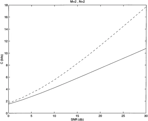
Fig. 1. Maximum mutual information achieved by2 2 2orthogonal design (6) compared to actual channel capacity for the M = 2, N = 2 system. Solid line: maximum mutual information for2 2 2orthogonal design. Dashed line: capacity of the M = 2, N = 2 system.
To see this, we compare the maximum mutual information
be-tween and in (10) with , the actual
channel capacity for the system.
As before, the maximum mutual information in (10) is simply the channel capacity for the structured channel matrix . De-noting this maximum mutual information by , we ob-tain
(12) The last equation implies that the orthogonal design (6) is re-strictive and does not allow us to achieve the full channel ca-pacity of the , system, but rather the capacity of
an , system at twice the SNR. Thus, when
we take a loss with the structure (6). The amount of this loss is substantial at high SNR and is depicted in Fig. 1 which shows the actual channel capacity compared to the maximum mutual information obtained by the orthogonal design (6).
For receive antennas, the analysis is similar and is omitted. We simply state that for transmit antennas and receive antennas the orthogonal design allows us
to attain only , rather than the full
.
3) Other Orthogonal Designs: The preceding subsection focuses on the orthogonal design but there are also
orthogonal designs for . The complex orthogonal
designs for are no longer “full-rate” (see [12]) and therefore generally perform poorly in the maximum mutual information they can achieve, even when . We give an example of these nonsquare orthogonal designs [12], [25].
For , we have, for example, the rate orthogonal
design
(13)
The factor ensures that . It can
be shown that maximum-likelihood estimation of the variables is decoupled. Again using an argument similar to
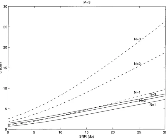
Fig. 2. Maximum mutual information achieved by4 2 3 orthogonal design (13) compared to actual channel capacity. Solid lines: maximum mutual information of4 2 3 orthogonal design for N = 1; 2; 3 receive antennas. Dashed lines: capacity of M = 3, N = 1; 2; 3 systems.
the one presented for , it is straightforward to show that the maximum mutual information attainable with (13) with
receive antennas is which is
(much) less than the true channel capacity . We
omit the proof and refer instead to Fig. 2 which shows the actual channel capacity compared to the maximum mutual information obtained by the orthogonal design (13).
B. Mutual Information Attainable With V-BLAST
We showed in Section II-A that, even though orthogonal de-signs allow efficient maximum-likelihood decoding and yield “full-diversity” (the appearance of the sum of the in the mutual information formulas attests to this), orthogonal designs generally cannot achieve high spectral efficiencies in a mul-tiple-antenna system, no matter how much coding is added to the transmitted signal constellation. This is especially true when the system has more than one receive antenna. An examination of the model (10) (and its counterparts for other orthogonal de-signs) reveals that the orthogonal design does not allow enough “degrees of freedom”—there are only two unknowns in (10) but four equations.
We can conclude that orthogonal designs are not suitable for very-high-rate communications. On the other hand, a scheme that is proven to be suitable for high spectral efficiencies is V-BLAST [7]. In V-BLAST each transmit antenna during each channel use sends an independent signal (often referred to as a
substream). Thus, over a block of channel uses, the transmit matrix takes on the form
..
. ... . .. ...
(14)
where each is an independent symbol drawn from a complex constellation. Since the transmitted symbols are not dispersed in time, is arbitrary. (We could, for example, take .)
When (the number of receive antennas is at least as large as the number of transmit antennas), there exist efficient schemes for decoding the V-BLAST matrices. These are based on “successive nulling and canceling” [7], and its more efficient variants [18], as well as more recently on sphere decoding [19]. All these decoding schemes essentially solve a well-conditioned system of linear equations. Successive nulling and canceling provides a fast approximate solution to the maximum-likeli-hood decoding problem with the benefit of cubic complexity in the number of transmit antennas . Sphere decoding, on the other hand, finds the exact maximum-likelihood estimate and benefits from avoiding an explicit exhaustive search. Recent work [20] has shown analytically that for a wide range of SNRs, the expected computational complexity of sphere decoding is also roughly cubic in the number of transmit antennas.
Because there is no restriction on the transmitted matrix in (14), the maximum mutual information that can be achieved by transmitting V-BLAST-like matrices is indeed the full mul-tiple-antenna channel capacity. Nevertheless, V-BLAST suffers from two deficiencies. First, nulling and canceling fails when there are fewer receive antennas than transmit antennas, since the decoder is confronted with an underdetermined system of linear equations. Although sphere decoding can still be used to find the maximum-likelihood estimate, the computational com-plexity is exponential in . Second, because V-BLAST transmits independent data streams on its antennas there is no built-in spatial or temporal coding, and hence none of the error resilience associated with such coding. We seek to remedy these deficiencies in the next section.
III. LINEAR-DISPERSIONSPACE–TIMECODES
In this section, we propose a high-rate coding scheme that retains the decoding simplicity of V-BLAST, handles any con-figuration of transmit and receive antennas, and has many of the coding advantages of schemes, such as the orthogonal designs, without suffering the loss of mutual information.
We call a linear-dispersion (LD) code one for which
(15)
where are complex scalars (typically chosen from
an -PSK or -QAM constellation) and where the and are fixed complex matrices. The code is completely de-termined by the set of dispersion matrices , whereas each individual codeword is determined by our choice of the
scalars .
We often find it more convenient to decompose the into their real and imaginary parts
and to write
(16)
where and . The dispersion
matrices also specify the code.2 The integer and
the dispersion matrices are, for the moment, unspecified.
Without loss of generality, we assume that and
have variance and are uncorrelated. Otherwise, we can always replace them with appropriate linear combina-tions that have this property—this simply leads to a
redefini-tion of the s and ’s. Thus, are unit-variance
and uncorrelated. Recall from our model in Section I-A that the
2We remark that it is also possible to defineA = jB and = ,
forq = 1; . . . ; Q, so that the LD codes become
S = A ; (17)
where the scalars are real.
transmit signal is normalized such that . This
induces the following normalization on the matrices : (18) The dispersion codes (16) subsume as special cases both or-thogonal designs and V-BLAST. For example, the
orthog-onal design (6) corresponds to and
(19)
whereas V-BLAST corresponds to and
(20)
where and are -dimensional and -dimensional
column vectors with one in the th and th entries, respec-tively, and zeros elsewhere.
Note that in V-BLAST each signal is transmitted from only one antenna during only one channel use. With the LD codes, however, the dispersion matrices potentially transmit some combination of each symbol from each antenna at every channel use. This can lead to desirable coding properties. Before we specify good choices of the dispersion matrices, we discuss decoding.
A. Decoding
An important property of the LD codes (16) is their linearity in the variables , leading to efficient V-BLAST-like decoding schemes. To see this, it is useful to write the block equation
(21) in a more convenient form. We decompose the matrices in (21) into their real and imaginary parts to obtain
We denote the columns of , , , , , and by
, , , , , and , and define
(22)
where . We then gather the equations in and
to form the single real system of equations
..
. ... ... (23)
where the equivalent real channel matrix is given by
..
. ... . .. ... ... (24)
We have a linear relation between the input and output vectors and
(25) where the equivalent channel is known to the receiver because the original channel , and the dispersion matrices
are all known to the receiver. The receiver simply uses (24) to find the equivalent channel. The system of equations between transmitter and receiver is not underdetermined as long as
(26) We may, therefore, use any decoding technique already in place for V-BLAST, such as successive nulling and canceling [7], its efficient square-root implementation [18], or sphere decoding [19]. The most efficient implementations of these schemes gen-erally require computations, and have roughly constant complexity in the size of the signal constellation [20]. B. Design of the Dispersion Codes
Although we have introduced the LD structure
we have not yet specified or the dispersion matrices
and . We have the inequality .
Intuitively, the larger is, the higher the maximum mutual information between and is since the matrix signal has more degrees of freedom. (Recall that orthogonal designs gen-erally have low mutual information because they do not have enough degrees of freedom.) On the other hand, the smaller
is, the more of a coding effect we obtain since the equivalent matrix becomes “skinnier” and the system of equations in (23) becomes more overdetermined. As a general practice, we
find it useful to take since this tends to
maximize the mutual information between and while still having the benefit of coding gain.3
We are left with the question of how to design the disper-sion matrices. We may first examine how sensitive the perfor-mance of the LD codes is to the choice of the dispersion ma-trices. Experiments with choosing random dispersion matrices subject to the normalization constraint (18), or the more strin-gent constraints
for
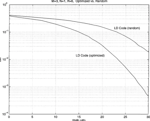
suggest that the performance for “average” is not gen-erally very good. Fig. 3 shows the bit-error rate of an , antenna system with randomly chosen versus optimized (according to a criterion we specify shortly) dispersion matrices. The difference is dramatic; it is important to choose the disper-sion matrices wisely.
One possible way of designing the spreading matrices is to study the pairwise probability of error of two different LD code-words, say
and
The worst case pairwise error is generally obtained when and
differ in only one element. We can then seek to choose the dispersion matrices that minimizes the probability of this error. The main drawback of this strategy is that it leads to a criterion on the individual columns of the matrix , rather than on the matrix in its entirety. Therefore, it is conceivable that designs based on this criterion could lead to a (near) singular , leading to other forms of errors. Finally, it is not clear what effect minimizing pairwise error probability has on the overall error probability, especially for a high-rate system. Therefore, this strategy for choosing the dispersion matrices does not appear to be promising.
We can also study the average pairwise error probability, ob-tained by choosing Gaussian in (25) and averaging the pair-wise error obtained between an independent and . We show in Appendix B that the average pairwise error has upper bound
pairwise (27)
We can then seek to minimize the upper bound with an
ap-propriate choice of and . Even
though (27) is a simple formula, suggesting that it can possibly be minimized, we do not attempt to do so here. The main reason is the following. Since multiple antennas are used for very high
3At high SNR, the capacity of the multiple-antenna system grows as
min(M; N) log , suggesting that we need K = min(M; N) degrees of freedom per channel use.
Fig. 3. Bit-error performance comparison for a random (fA ; B g drawn from a complex Gaussian distribution and normalized) and an optimized LD code for M = 3 transmit and N = 1 receive antenna for T = Q = 4, and rate R = 6 bits/channel use (obtained by transmitting 64-QAM on s ; . . . ; s ).
rates, the pairwise error probability for any two signals is ex-tremely small. In Section I-A we argue that even for the small
test-case of transmit and receive antennas, we
could theoretically have a constellation size of as many as signal-matrices at 20 dB. It is therefore conceivable that the pairwise error probability between any two could be roughly . Trying to minimize a quantity such as (27) that is already so small can be numerically quite difficult.
Fortunately, information theory suggests a natural alternative that is connected with minimizing (27) but is more fundamental. Recall from Section II-A that orthogonal designs are deficient in the maximum mutual information they support for
or . We therefore choose to maximize the
mu-tual information between and in (23). This guarantees that we are taking the smallest possible mutual information penalty within the LD structure (16). We propose to design codes that are “blessed” by the “logdet” formula (3).
We formalize the design criterion as follows.
The Design Method
1) Choose (typically, ).
2) Choose that solve the optimization problem
(28)
for an SNR of interest, subject to one of the following constraints:
i)
ii) ,
iii) ,
where is given by (24) with the having independent entries.
Note that (28) is effectively (3) with ; as mentioned in Section III, we may take the entries of (the ’s and ’s) to be uncorrelated with variance . Moreover, because the real and imaginary parts of the noise vector in (23) also have variance , the SNR remains . We also note that (28) differs from (3) by the outside factor because the effective channel is real-valued and the LD code spans channel uses.
We now make some remarks.
1) Clearly, .
2) The problem (28) can be solved subject to any of the con-straints i)–iii). Constraint i) is simply the power constraint
(18) that ensures . Constraint ii) is more
restrictive and ensures that each of the transmitted signals and are transmitted with the same overall power from the antennas during the channel uses. Finally, constraint iii) is the most stringent, since it forces the sym-bols and to be dispersed with equal energy in all spatial and temporal directions.
3) Since constraints i)–iii) are successively more restric-tive, the corresponding maximum mutual informations obtained in (28) are necessarily successively smaller. Nevertheless, we have found that constraint iii) generally imposes only a small information-theoretic penalty while having the advantage of better coding (or diversity) gains. Using symmetry arguments one may conjecture that the optimal solution to the problem with constraint i) should automatically satisfy constraint ii). But we have not experimented sufficiently with constraint i) to confirm this; we instead usually restrict our attention to constraints ii) and iii). We have empirically found that of two codes with equal mutual informations, the one satisfying the more stringent constraint gives lower error rates. Examples of this phenomenon appear in Section IV. 4) The solution to (28) subject to any of the constraints i)–iii)
is highly nonunique: simply reordering the
gives another solution, as does pre- or post-multiplying all the matrices by the same unitary matrix. However, there is also another source of nonuniqueness which is more subtle. Equation (23) shows that we can always pre-mul-tiply the transmit vector
by a orthogonal matrix to obtain a new
vector with
en-tries that are still independent and -distributed. Thus, we may rewrite (23) as
Defining , , and as in (22) allows us to write
the new equivalent channel as shown in (29)
at the bottom of the page. Since the entries of and have the same joint distribution, the maximum mutual information obtained from the equivalent channels and are the same. This implies that the transformation from
the dispersion matrices to
(30)
where is an orthogonal matrix,
pre-serves the mutual information. Thus, the transformation (30) is another source of nonuniqueness to the solution of (28).
This nonuniqueness can be used to our advantage because a judicious choice of the orthogonal matrix allows us to change the dispersion code through the transformation (30) to satisfy other criteria (such as space–time diversity) without sacrificing mutual infor-mation. Examples of this appear in Remark 7, where we
construct unitary from the rank-one V-BLAST
dispersion matrices (20), and in Section IV in some of the two and three-antenna LD code constructions. 5) The constraints i)–iii) are convex in the dispersion
ma-trices since they can be rewritten as i′)
ii′) ,
iii′) ,
all of which are convex. However, the cost function is neither concave nor
convex in the variables . Therefore, it is
possible that (28) has local maxima. Nevertheless, we have been able to solve (28) with relative ease using gradient-based methods and it does not appear that local maxima pose a great problem. Table I in Section IV-A gathers the maximum mutual informations obtained via gradient-ascent for a variety of different , , and . The results show that maximum mutual informations obtained are quite close to the Shannon capacity (which is clearly an upper bound on what can be achieved) and so they suggest that the values obtained, if not the global maxima, are quite close to them. (For convenience, we include the gradient of the cost function (28) in Appendix A.)
..
. . .. ... ... . .. ...
..
6) We know that for , , , one solution to (28), for any of the constraints i)–iii), is the orthogonal design (19). This holds simply because the mutual infor-mation of this particular orthogonal design achieves the
actual channel capacity . We note
that there are also many other solutions that work equally well.
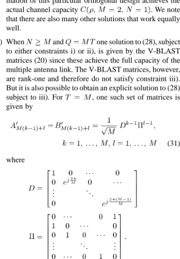
7) When and one solution to (28), subject
to either constraints i) or ii), is given by the V-BLAST matrices (20) since these achieve the full capacity of the multiple antenna link. The V-BLAST matrices, however, are rank-one and therefore do not satisfy constraint iii). But it is also possible to obtain an explicit solution to (28) subject to iii). For , one such set of matrices is given by (31) where .. . . .. .. . . .. ...
The above code can be constructed by starting with the V-BLAST matrices (20) and applying the transformation (30) with a suitable . We do not give the full here, and only mention that, for , the transformation is
with similar expressions for the . It can be readily checked that the matrix constructed from the
coef-ficients relating to is orthogonal.
Fig. 4 in Section IV presents a performance comparison of the LD code (31) with V-BLAST.
8) The block length is essentially also a design variable. Although it must be chosen shorter than the coherence time of the channel, it can be varied to help the optimiza-tion (28). We have found that choosing
often yields good performance.
9) Although the SNR is a design variable, we have found that the optimization (28) is not sensitive to its value for large ( 20 dB). Once the optimization is performed, the resulting LD code generally works well over a wide range of SNRs.
10) It does not appear that (28) has a simple closed-form solution for general , , , although we see in Sec-tion IV that, in some nontrivial cases, it can lead to lutions with simple structure. We have found that the so-lution to (28) often yields an equivalent channel matrix that is “as orthogonal as possible.” Although complete orthogonality appears not always to be possible, our ex-perience with optimizing (28) shows that the difference can be made quite small with a proper choice of and (see Table I in Sec-tion IV-A). Thus, there appears to be very little capacity penalty in assuming the LD structure (16).
11) When the equivalent channel matrix is orthogonal, maximum-likelihood decoding and the V-BLAST-like nulling/canceling [7] perform equally well because the
estimation errors of are decoupled.
12) The design criterion (28) depends explicitly on the number of receive antennas , both through the choice of and through the matrix in (24). Hence, the optimal codes, for a given , , and , are different for different .
Nevertheless, a code designed for receive antennas can also easily be decoded using nulling/canceling or
sphere decoding with antennas. Hence, if we
wish to broadcast data to more than one user, we may use a code designed for the user with the fewest receive antennas, with a rate supported by all the users.
13) The ultimate rate of the code depends on the number of signals sent , the block length of the code , and the size
of the constellation from which are chosen.
We assume that the constellation is -PSK or -QAM. Then the rate in bits per channel use is easily seen to be
(32)
14) A standard gray-code assignment of bits to the symbols of the -PSK or -QAM constellation may be used. 15) We see that the average pairwise error probability (27)
and the design criterion (28) have a similar expression. By interchanging the expectation and log in (28), we see that maximizing (28) has some connections to minimizing (27).
On the other hand, our design criterion is not directly connected with the diversity design criterion given in [9] and [10], which is concerned with maximizing
(33) A constellation attains full diversity if (33) is nonzero. This criterion depends only on matrix pairs, and there-fore does not exclude matrix designs with low spectral efficiencies.
At high spectral efficiencies, the number of signals in the constellation of possible matrices is roughly ex-ponential in the channel capacity at a given SNR. This number can be very large—in Section IV we present a
code for and that effectively has matrices. The relation between the diversity criterion and the performance of such a large constellation is very tenuous. Even if
for many pairs of , our probability of encountering one of these matrices may still be exceedingly small, and the constellation performance may still be excellent. For such a large constellation it is probably more important for the matrices in this constellation to be distributed in the space of matrices according to the distribution that at-tains capacity; the mutual information criterion attempts to achieve this distribution.
As the SNR is allowed to increase, the performance of some given space–time code with some given rate be-comes more dependent on the diversity criterion since making a decoding error to a “nearest neighbor” becomes relatively more important. Chernoff bound computations in [10] show that the pairwise error falls off as , where is the rank of . However, by increasing the SNR and keeping the code (and hence rate) fixed, we are effectively reducing the relative spectral efficiency of the code as compared with the channel capacity. We are there-fore led again to the conclusion that diversity plays a sec-ondary role at high spectral efficiencies. In Section IV, we present a comparison of codes that satisfy various combi-nations of the mutual information and diversity criteria. The code that satisfies both criteria performs best, fol-lowed by the mutual information criterion only, folfol-lowed by the diversity criterion only.
16) Although the dispersion matrices can, in gen-eral, be complex, we have found that constraining them to be real imposes little, if any, penalty in the optimized mutual information.
17) Our mutual information calculations and design exam-ples assume that the channel matrix has independent entries, but designs for other channel distribu-tions using the mutual information criterion are also pos-sible.
IV. EXAMPLES OFLD CODES ANDPERFORMANCE
In this section, we present simulations that compare the per-formance of LD codes to V-BLAST and orthogonal designs over a wide range of SNRs and various combinations of receive and transmit antennas. All the LD codes are designed for a target SNR of 20 dB (see Remark 9 in Section III-B).
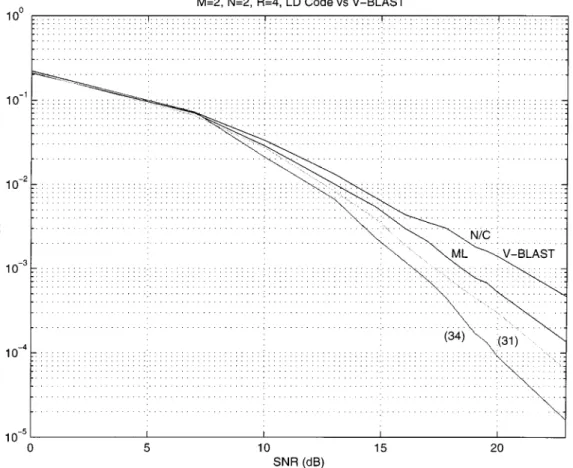
LD Versus V-BLAST : , ,
We look first at an , system at rate and
compare V-BLAST with an LD code. In V-BLAST, ,
and the matrices are given by (20). To design an LD code we also choose but use the matrices given by (31) that satisfy constraint iii) in (28). To achieve , we transmit quaternary phase-shift keying (QPSK) on . The re-sults can be seen in Fig. 4, where the bit errors are compared. Even though both V-BLAST and the LD code support the full channel capacity, which is 11.28 bits/channel use at SNR 20 dB, the LD code has better performance; this can probably be attributed to the spatial and temporal dispersion of the symbols that V-BLAST lacks.
Since we are transmitting at a rate our spectral efficiency is low relative to the channel capacity, and we may therefore anticipate significant coding advantages from also satisfying the diversity criterion (33)—see Remark 15 in Section III-B for an explanation of the relative importance of diversity at low spectral efficiencies. The LD code (31) may be modified as in Remark 4 in Section III-B, without changing its mutual information, by premultiplying the transmitted signal vector by an orthogonal matrix . In [26], a two-antenna code is designed using the full diversity criterion. This code also happens to support the full capacity of the channel, and we may put it into our LD code framework by choosing to be the block-diagonal matrix shown in (34) at the bottom of the page (where the subscript “ ” denotes real part, and “ ” denotes
imaginary part) and where and . The result is
a code that satisfies both the mutual information criterion and diversity criterion; it is also displayed in Fig. 4 and has the best performance. Although the codes in the figure all satisfy the mutual information condition, the importance of also satisfying the diversity criterion at relatively low spectral efficiencies is underscored. The next example shows that satisfying the mutual information condition is most important at higher spectral efficiencies.
LD Versus OD: ,
We show in Section II-A2 that the orthogonal design is deficient in mutual information when . This deficiency should be reflected in its performance with . We test its
performance when at versus the LD code
given by (31) for and . The result can be seen
in Fig. 5 which clearly shows the better performance of the LD code over a wide range of SNRs. To achieve , we see from (32) that the orthogonal design needs to choose and from a 256-QAM constellation, while the LD code can choose from a 16-QAM constellation because it has four symbols . We note that the orthogonal design has good diversity (33) [12]
Fig. 4. The upper two curves are the bit error performance of V-BLAST (20) with nulling/canceling (upper), and with maximum-likelihood decoding (lower). The lower two curves are the LD code given by (31) forM = N = T = 2 and Q = 4 (upper) and the code (34) with = e (lower). For both these codes, sphere decoding is used to find the maximum-likelihood estimates. The rate isR = 4, and is obtained by transmitting QPSK on s ; . . . ; s .
but achieves only 7.47-bits/channel use mutual information at 20 dB, while the LD code achieves the full channel capacity of 11.28 bits/channel use. The orthogonal design and LD code are maximum-likelihood decoded (using the sphere decoder in the case of the LD code). The orthogonal design is easier to de-code than the LD de-code because and may be decoded sep-arately, and its performance is better for SNR 35 dB (where spectral efficiency is low compared with capacity).
But we may obtain a code that is uniformly better at all SNRs by using (34) to improve the diversity of (31) without changing its mutual information. As shown in [26], setting
is a good choice when transmitting 16-QAM. The performance of this constellation is also shown in Fig. 5. Its performance is better than the unmodified LD code at high SNR. Clearly, the best code satisfies both the mutual information and diversity criteria, if possible.
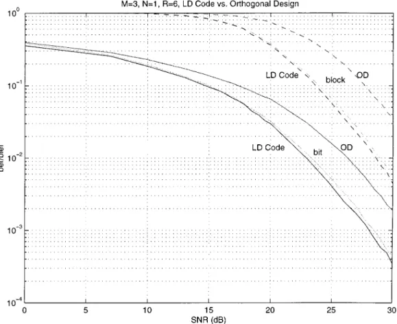
LD Versus OD: , ,
We present a code for transmit antennas and receive antennas and compare it with the orthogonal design pre-sented in Section II-A3 with block length . The orthog-onal design (13) is written in terms of and as
(35)
It turns out that this orthogonal design is a local maximum to
(28) for and . It achieves a mutual information
of 5.13 bits/channel use at 20 dB, whereas the channel capacity is 6.41 bits/channel use.
To find an LD code with the same block length, we first
ob-serve that must obey the constraint , with
and . Therefore, , and to obtain the highest possible mutual information we choose . After optimizing (28) using a gradient-based search (Appendix A) and converging to a local maximum at 20 dB, we find (36) as shown at the bottom of the following page. This code has a mutual informa-tion of 6.25 bits/channel use at 20 dB, which is most of the channel capacity. The matrix has some interesting features. First, it has orthogonal (but not orthonormal) columns; second, its corresponding matrix is nonzero in only 12 of its 56 off-diagonal entries.
Fig. 6 compares the performance of the orthogonal design (35) with the LD code (36) at rate . (From (32), the
rate of either code is ; we achieve by
having the orthogonal design send 256-QAM, and the LD code send 64-QAM.) The decoding in both cases is maximum like-lihood, which in the case of the LD code is accomplished with the sphere decoder, and in the case of the orthogonal design is simple because are decoupled. We also compare de-coding with nulling/canceling, which appears to be only slightly worse than maximum likelihood (this is perhaps because the columns of the LD code are orthogonal—see Remark 11 in
Fig. 5. Bit error performance of the2 2 2 orthogonal design (19) and the LD code given by (31) for M = N = T = 2 and Q = 4 (dashed line) and the code (34) with = e (lower solid line). The rate isR = 8 implying that the orthogonal design transmits 256-QAM whereas the LD codes transmit 16-QAM. The decoding is maximum likelihood in both cases.
Section III-B). We see from Fig. 6 that the LD code performs uniformly better.
, LD Code From Orthogonal Dessign
The , , LD code (36) is obtained via
a gradient search and has mutual information 6.25 bits/channel use at 20 dB. However, this is less than the full , capacity of , and we would like to close the gap a little. We should be able to make an LD code with mutual information at least as large as the mutual information of the two-antenna orthogonal design (6), which is . We do not resume our gradient search since the value appears to be a local maximum, but rather try a slightly different approach. We begin with the two-antenna orthogonal design and create a three-antenna LD code that preserves its mutual information.
One possible code is obtained by symmetrically concate-nating three orthogonal designs (normalized to obey the power constraint)
(37)
When viewed as an LD code, (37) has the deficiency that and are only nonzero for two-channel uses and not for the full six-channel uses. Moreover, and have rank two, rather
Fig. 6. Block (dashed) and bit (solid) error performance of orthogonal design (35) and the LD code (36) forM = 3 antennas. The rate is R = 6 bits/channel use, obtained in the orthogonal design by transmitting 256-QAM ons ; . . . ; s and obtained in the LD code by transmitting 64-QAM on s ; . . . ; s . The uppermost block and bit curves are the orthogonal design, decoded with maximum likelihood. The lower two block and bit curves (very close to one another) are the LD code decoded with nulling/canceling (upper) and maximum likelihood (lower). The comparison of block error is meaningful here because the block size in all cases is T = 4.
than their full possible rank of three. Consequently, constraint iii) in Section III-B is not satisfied, and as we point out in Re-mark 3, of two codes that have the same mutual information, the one satisfying the stronger constraint generally performs better. It is clear that the code (37) is really only a two-antenna code in crude disguise and performs worse than (36), even though its mutual information is slightly higher.
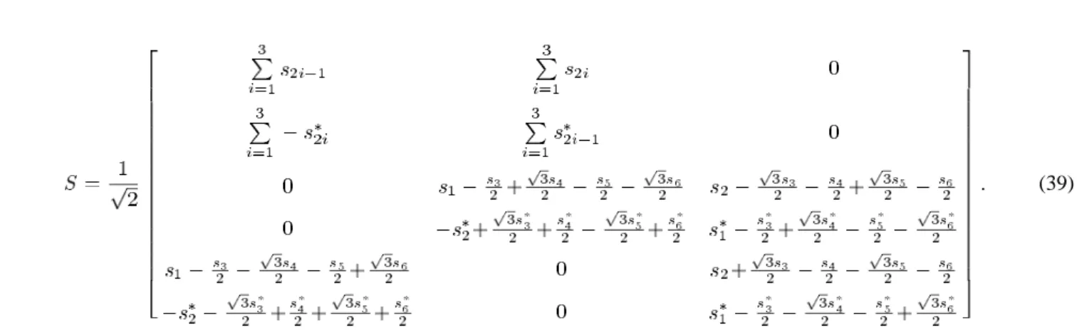
To improve its performance, we seek to modify it so that con-straint iii) is satisfied without changing its mutual information. One possible modification is described in Remark 4 in Sec-tion III-B. (See, in particular, the transformaSec-tion involving (30).) Let denote the discrete Fourier transform (DFT) matrix, and choose to be the real orthogonal matrix
ob-tained by replacing each element of by the
real matrix . The transformation of
to new dispersion matrices is
(38)
The resulting matrix is shown in (39) at the bottom of the following page. Each dispersion matrix spans all six channel
uses and is unitary . Thus, constraint
iii) is satisfied. Because the transformation (38) is a special case
of the transformation (30), the mutual information is still 6.28 bits/channel use ( 20 dB).
We see in Fig. 7 that this code performs very well: displayed is (37) (which has the same performance as the orthog-onal design) and the LD codes (36) and (39) for rate . (The symbol constellation is hence QPSK.) The code (37) has the worst performance. The LD code (36) with
has better performance, despite its lower mutual information, because it satisfies constraint iii). The best performer, however, is (39), because its mutual information is higher than (36) ( versus ), it satisfies constraint iii), and perhaps also because it has a longer block length ( versus ).
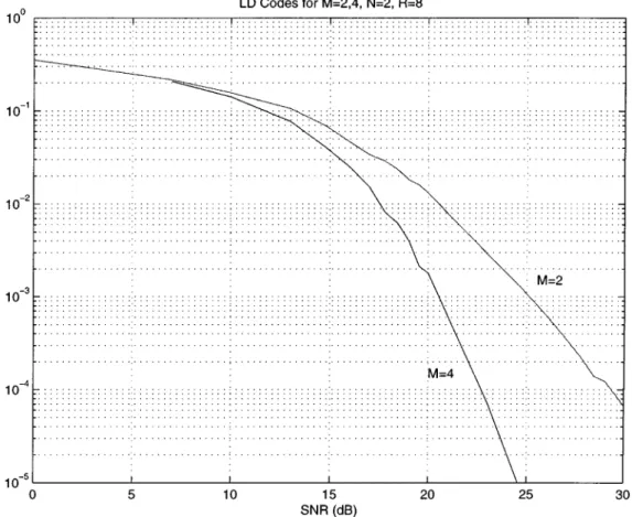
Two LD Codes: , ,
Fig. 8 demonstrates the dramatic improvement of increasing
the number of transmitter antennas from to with
. An LD code was designed for , , and
that attains 11.84 bits/channel use at SNR 20 dB, whereas the channel capacity is 12.49 bits/channel use. We do not explicitly present the code because and there are therefore 24 and matrices. (The reader may obtain the code by contacting the authors.) We compare this code with the best LD code we have for transmit antennas ((31)
Fig. 7. Bit error performance forM = 3, N = 1, and R = 2. The top curve is (37), whose performance is identical to a 2 2 2 orthogonal design. The middle curve is theT = 4 LD code (36), and the lower curve is the T = 6 LD code (39). In all cases, the transmitted symbols are QPSK, decoded via maximum likelihood.
LD Code: , ,
The last example is an LD code for and at
rate 16 bits/channel use displayed in Fig. 9. It is worth
noting that the capacity of an , system at 20 dB
is 24.94-bits/channel use. We therefore restrict our attention in this figure to relatively high SNR. The LD code was designed using gradient search applied to (28) until a local maximum was obtained at 20 dB. The code attains a mutual information
of 23.10-bits/channel use, with and has . To
obtain , we choose from a 16-QAM
con-stellation. Because of the sheer number of matrices involved, we again do not explicitly present the LD code here. We
in-clude this example to demonstrate that very high rates are well within the reach of these codes, even with maximum-likelihood decoding. The figure compares the performance of nulling/can-celing versus maximum-likelihood decoding with the sphere de-coder, and maximum likelihood performs far better. It is remark-able that the sphere decoder succeeds at all in obtaining the max-imum-likelihood estimate, since a full exhaustive search would
need to examine hypotheses.
A. Table of Mutual Informations
Table I summarizes the mutual informations of some LD codes that we generated, including the examples from the
Fig. 8. Bit error performance of the best LD code forT = M = N = 2 and Q = 4 ((31) modified with (34)) and an LD code for T = 6, M = 4, and N = 2. The rate isR = 8 and is obtained by transmitting 16-QAM on each symbol. The decoding in both cases is maximum likelihood. The LD code for M = 4 achieves 11.84 bits/channel use mutual information at = 20 dB versus the channel capacity of 12:49, and benefits dramatically from the two extra transmit antennas.
TABLE I
MUTUALINFORMATIONC (; T; M; N) OBTAINED VIA GRADIENT-ASCENTOPTIMIZATION OF THECOSTFUNCTION(28), COMPARED TO THE ACTUALCHANNELCAPACITYC(; M; N)FORDIFFERENTVALUES OFM
ANDNATSNR = 20 dB
previous section, and the actual channel capacities at
20 dB. As can be observed, is very close to
; there is little penalty in the linear structure of the dispersion codes. When studying this table, we should bear in
mind that the entries for are not necessarily
the best achievable since (28) was maximized via gradient ascent. Our maxima are therefore quite possibly local.
Further-more, the values of are for codes with block
lengths obeying . Conceivably, increasing
could also yield higher values for .
V. CONCLUSION
The linear dispersion codes we have introduced are simple to encode and decode, apply to any combination of transmit
and receive antennas, subsume as special cases many earlier space–time transmission schemes, and satisfy an information-theoretic optimality property. We have argued that codes that are deficient in mutual information can never be used to attain capacity. We also have shown that information-theoretic opti-mality has a theoretical connection with low pairwise error prob-ability and good performance at high spectral efficiencies. The LD codes are designed to be linear while having little (if any) penalty in mutual information, and additional channel coding
across can be combined with an LD code to attain
most (if not all) of the channel capacity.
We have given some specific examples of the LD codes, and presented a recipe for generating more codes within this linear structure for any combination of transmit and receive antennas. Our simulations indicate that codes generated with this recipe compare favorably with existing space–time schemes in their good performance and low complexity. We have argued that the diversity criterion commonly used to design space–time codes plays a secondary role to mutual information criterion at high spectral efficiencies. The diversity criterion alone may lead to code designs that cannot attain capacity.
In our simulations, we decoded the LD codes by either max-imum likelihood or by nulling and canceling. Because of the linear relation between and in (25), the maximum-likeli-hood search could be accomplished efficiently using the sphere decoding algorithm, which, for SNRs of interest, has polyno-mial complexity in the number of antennas.
Fig. 9. Bit error performance of an LD code forM = 8 and N = 4 with Q = 32 with nulling/canceling (upper curve) and maximum-likelihood decoding (lower curve). The rate isR = 16 and is obtained by transmitting 16-QAM on each symbol. The LD code achieves mutual information 23.10-bits/channel use at = 20 dB versus the channel capacity of 24:94.
We have used the average capacity (across different channel realizations) as our design metric, rather than an outage capacity (for one-channel realization), because channels are rarely static for very long and because the outage capacity does not have a simple closed-form expression. It is reasonable to expect that codes that work well on average should also help reduce the probability of outage events, but this remains to be explored.
It would be interesting to see if the LD codes that satisfy (28) possess any general algebraic structure. This would lead to better theoretical understanding of the codes, as well as to possibly faster and better decoding algorithms. The codes (36) and (39), for example, are local maxima of the cost function and yet have simple structure. It would also be important to
charac-terize theoretically how close can be made
to —what is the penalty incurred by the LD
struc-ture? Our experience suggests that the penalty is small. Perhaps the penalty approaches zero as ?
Finally, there are potentially many ways to optimize the cost function (28), and the gradient method we chose is only one of them. More sophisticated optimization techniques may also be useful.
APPENDIX A
THEGRADIENTCOMPUTATION
In all the simulations presented in this paper, the maxi-mization of the cost function in (28), needed to design the LD codes, is performed using a simple constrained-gradient-ascent method. In this appendix, we compute the gradient of the cost function in (28) that this method requires. More sophisticated optimization techniques that we do not consider, such as Newton–Raphson, scoring, and interior-point methods, can also use this gradient.
To help compute this gradient, we rewrite the cost function in (28) as shown in (A1) at the bottom of the page, where ,
, and are defined in (22) for and
.
We wish to compute the gradient of the cost function in (A1)
with respect to the spreading matrices , , , and
. To simplify the gradient calculation, we assume the log-arithm in (A1) is base . The gradient with respect to is computed here explicitly—the remaining three gradients follow similar arguments and are given at the end of the section.
..
The th entry of the gradient of a function is
(A2)
where and are the -dimensional and -dimensional
unit column vectors with one in the th and th entries, respectively, and zeros elsewhere. Defining the matrix
appearing in the of (A1) as , so that
; we then obtain
..
. . .. ...
..
. ... ... . .. ...
transpose higher order terms. (A3)
Applying yields (A4), shown at the
bottom of the following page, where in the last step we use . This now leads to
..
. . .. ...
..
. ... ... . .. ...
..
. . .. ...
..
. ... ... . .. ...
..
. . .. ...
(A5)
where we have defined the matrix as
..
. ... . .. ...
(A6) This concludes the gradient calculation with respect to .
Similar expressions can be found for the gradients with
re-spect to , , and . With
..
. ... . .. ...
(A7) these gradients are
(A8)
(A9)
(A10)
(A11)
APPENDIX B
AVERAGEPAIRWISEPROBABILITY OFERROR
The signal model (25) is
where is a given real matrix. We compute the
pairwise error by conditioning on
We assume that two independent signal vectors and are chosen with entries from independent zero-mean real Gaussian densities with variance . The entries of the
additive noise vector are also chosen from this
density. We want the probability that a maximum-likelihood decoder mistakes for , given that is transmitted, averaged over and , and conditioned on .
Because has a Gaussian distribution, we equivalently want
pairwise
transmitted
(B12)
(B13)
Equation (B12) follows because and are independent Gaussian vectors and we have replaced the difference of the two vectors by a single vector with twice the variance.
To compute (B13), we look at the characteristic function of the scalar
We can write
The characteristic function of is
We use the formula
for positive real , where is a real vector,
to conclude that
This implies that pairwise
(B14)
..
. . .. ... ... ... ... . .. ...
transpose higher order terms
..
. . .. ... ... ... ... . .. ...
We wish to switch the order of integration, and we have to make sure that is well-behaved as a function of and . We can ensure its good behavior by shifting the path of integration to . (The formal argument for why this does not affect the value of the integral is omitted.) We obtain
pairwise
(B15)
We now compute by first computing the
eigen-values of . The eigenvalues of are the solutions to
as a polynomial in . Using a standard determinant identity [27], we can write this equation as
where are the eigenvalues of . Solving
this last equation yields zero eigenvalues, with the remaining eigenvalues given by
Therefore,
and (B15) becomes pairwise
(B16) To get an upper bound on the pairwise error probability, we ignore the second appearance of in (B16) to obtain
pairwise
It follows that
pairwise (B17)
Applying a union bound to this average pairwise probability of error yields an upper bound on probability of error of a signal constellation. Suppose that the transmission rate is , so that there are elements in our constellation for ; then
REFERENCES
[1] G. J. Foschini, “Layered space–time architecture for wireless commu-nication in a fading environment when using multi-element antennas,”
Bell Labs. Tech. J., vol. 1, no. 2, pp. 41–59, 1996.
[2] I. E. Telatar, “Capacity of multi-antenna Gaussian channels,” Europ.
Trans. Telecommun., vol. 10, pp. 585–595, Nov. 1999.
[3] A. Wittneben, “Basestation modulation diversity for digital simulcast,” in Proc. IEEE Vehicular Technology Conf., 1991, pp. 848–853. [4] N. Seshadri and J. Winters, “Two signaling schemes for improving the
error performance of frequency-division-duplex (fdd) transmission sys-tems using transmitter antenna diversity,” in Proc. IEEE Vehicular
Tech-nology Conf., 1993, pp. 508–511.
[5] A. Wittneben, “A new bandwidth-efficient transmit antenna modulation diversity scheme for linear digital modulation,” in Proc. IEEE Int.
Com-munications Conf., 1993, pp. 1630–1634.
[6] J. Winters, “The diversity gain of transmit diversity in wireless systems with Rayleigh fading,” in Proc. IEEE Int. Communications Conf., 1994, pp. 1121–1125.
[7] G. D. Golden, G. J. Foschini, R. A. Valenzuela, and P. W. Wolniansky, “Detection algorithm and initial laboratory results using V-BLAST space–time communication architecture,” Electron. Lett., vol. 35, pp. 14–16, Jan. 1999.
[8] G. J. Foschini, G. D. Golden, R. A. Valenzuela, and P. W. Wolniansky, “Simplified processing for high spectral efficiency wireless communi-cation employing multi-element arrays,” J. Select. Areas Commun., vol. 17, pp. 1841–1852, Nov. 1999.
[9] J.-C. Guey, M. P. Fitz, M. R. Bell, and W.-Y. Kuo, “Signal design for transmitter diversity wireless communication systems over Rayleigh fading channels,” in Proc. IEEE Vehicular Technology Conf., 1996, pp. 136–140.
[10] V. Tarokh, N. Seshadri, and A. R. Calderbank, “Space–time codes for high data rate wireless communication: Performance criterion and code construction,” IEEE Trans. Inform. Theory, vol. 44, pp. 744–765, Mar. 1998.
[11] S. M. Alamouti, “A simple transmitter diversity scheme for wireless communications,” IEEE J. Select. Areas Commun., pp. 1451–1458, Oct. 1998.
[12] V. Tarokh, H. Jafarkhani, and A. R. Calderbank, “Space–time block codes from orthogonal designs,” IEEE Trans. Inform. Theory, vol. 45, pp. 1456–1467, July 1999.
[13] B. M. Hochwald and T. L. Marzetta, “Unitary space–time modulation for multiple-antenna communication in Rayleigh flat fading,” IEEE Trans.
Inform. Theory, vol. 46, pp. 543–564, Mar. 2000.
[14] B. Hochwald and W. Sweldens, “Differential unitary space time mod-ulation,” IEEE Trans. Commun., vol. 48, pp. 2041–2052, Dec. 2000. [Online] Available: http://mars.bell-labs.com.
[15] B. Hughes, “Differential space–time modulation,” IEEE Trans. Inform.
Theory, pp. 2567–2578, Nov. 2000.
[16] A. Shokrollahi, B. Hassibi, B. Hochwald, and W. Sweldens, “Represen-tation theory for high-rate multiple-antenna code design,” IEEE Trans.
Inform. Theory, vol. 47, pp. 2335–2367, Sept. 2001. [Online] Available:
http://mars.bell-labs.com.
[17] V. Tarokh and H. Jafarkhani, “A differential detection scheme for transmit diversity,” J. Select. Areas Commun., pp. 1169–1174, July 2000.
[18] B. Hassibi, “An efficient square-root algorithm for BLAST,” IEEE
Trans. Signal Processing. [Online] Available: http://mars.bell-labs.com,
submitted for publication.
[19] M. O. Damen, A. Chkeif, and J.-C. Belfiore, “Lattice code decoder for space–time codes,” IEEE Commun. Lett., vol. 4, pp. 161–163, May 2000.
[20] B. Hassibi and H. Vikalo, “On the expected complexity of sphere de-coding,” in preparation.
[21] B. Hassibi and B. Hochwald, “How much training is needed in mul-tiple-antenna wireless links?,” IEEE Trans. Inform. Theory. [Online] Available: http://mars.bell-labs.com, submitted for publication. [22] T. Marzetta, B. Hassibi, and B. Hochwald, “Structured unitary
space–time autocoding constellations,” IEEE Trans. Inform. Theory, vol. 48, pp. 942–950, Apr. 2002.
[23] B. Hassibi and B. Hochwald, “High-rate linear space–time codes,” in
Proc. 38th Allerton Conf. Communications, Control and Computing,
Oct. 2000, pp. 1047–1056.
[24] S. Sandhu and A. Paulraj, “Space–time block codes: A capacity perspec-tive,” IEEE Commun. Let., vol. 4, pp. 384–386, Dec. 2000.
[25] G. Genesan and P. Stoica, “Space–time diversity using orthogonal and amicable orthogonal designs,” in Proc. Int. Conf. Accoustics, Speech and
Signal Processing, 2000, pp. 335–338.
[26] M. O. Damen, A. Tewfik, and J.-C. Belfiore, “A construction of a space–time code based on the theory of numbers,” IEEE Trans. Inform.
Theory, submitted for publication.
[27] T. Kailath, A. Sayed, and B. Hassibi, Linear Estimation. Englewood Cliffs, NJ: Prentice-Hall, 2000.