Price discrimination through communication
∗Itai Sher† Rakesh Vohra‡ May 26, 2014
Abstract
We study a seller’s optimal mechanism for maximizing revenue when a buyer may present ev-idence relevant to her value. We show that a condition very close to transparency of buyer segments is necessary and sufficient for the optimal mechanism to be deterministic–hence akin to classic third degree price discrimination–independently of non-evidence characteristics. We also find another sufficient condition depending on both evidence and valuations, whose content is that evidence is hierarchical. When these conditions are violated, the optimal mechanism contains a mixture of second and third degree price discrimination, where the former is imple-mented via sale of lotteries. We interpret such randomization in terms of the probability of negotiation breakdown in a bargaining protocol whose sequential equilibrium implements the optimal mechanism.
JEL Classification: C78, D82, D83.
Keywords: price discrimination, communication, bargaining, commitment, evidence, network flows.
1
Introduction
This paper examines the problem of selling a single good to a buyer whose value for the good is private information. The buyer, however, is sometimes able to support a claim about her value with
∗
A previous version of this paper circulated under the title “Optimal Selling Mechanisms on Incentive Graphs”. We are grateful to Melissa Koenig and seminar participants at The Hebrew University of Jerusalem, Tel Aviv University, the Spring 2010 Midwest Economic Theory Meetings, 2010 Econometric Society World Congress, 2011 Stony Brook Game Theory Festival, Microsoft Research New England, 2012 Annual Meeting of the Allied Social Sciences Associations, the Universit´e de Montr´eal, 2011 Canadian Economic Theory Conference, and the 2014 SAET Conference on Current Trends in Economics. We thank Johannes Horner and two anonymous referees for their helpful comments. Itai Sher gratefully acknowledges a Grant-in-Aid and Single Semester Leave from the University of Minnesota. All errors are our own.
†
Economics Department, University of Minnesota. Email: [email protected].
‡
Department of Economics and Department of Electrical and Systems Engineering, University of Pennsylvania. Email: [email protected].
evidence. Evidence can take different forms. For example, evidence may consist of an advertisement showing the price at which the consumer could buy a substitute for the seller’s product elsewhere. It is not essential that a buyer present a physical document; a buyer who knows the market–and hence knows of attractive outside opportunities–may demonstrate this knowledge through her words alone, whereas an ignorant buyer could not produce those words.
Our model is relevant whenever a monopolist would like to price discriminate on the basis of membership in different consumer segments but disclosure of membership in a segment isvoluntary. This is the case with students, senior citizens, AAA members, and many other groups. Moreover, consumer segments often overlap (e.g., many AAA members are senior citizens). If the seller naively sets the optimal price within each segment without considering that consumers in the overlap will select the cheapest available price, she implements a suboptimal policy. So an optimal pricing policy must generally account for the voluntary disclosures that pricing induces.
Our model allows the monopolist not only to set prices conditional on evidence, but to sell lotteries that deliver the object with some probability. Probabilistic sale can be interpreted as delay or quality degradation.1 Thus, our model entails a mixture of second and third degree price discrimination. Evidence and, moreover, voluntary presentation of evidence play a crucial role in generating the richness of the optimal mechanism. In the absence of all evidence, the optimal mechanism is a posted price. When segments are transparent to the seller, which corresponds to the case where evidence disclosure is non-voluntary or where all consumers can prove membership
and the lack of it for all segments, the optimal mechanism in our setting is standard third degree price discrimination. More generally, segments may not be transparent, and some consumers may not be able to prove that they do not belong to certain segments. For example, how does one prove that one is not a student? In this case, the optimal mechanism must determine prices for lotteries as a function of submitted evidence. The same lottery may sell to different types for different prices. The allocation need not be monotone in buyers’ values in the sense that higher value types may receive the object with lower probability than lower value types. This can be so even when the higher value type possesses all evidence possessed by the lower value type.
We organize the analysis of the problem via the notion of an incentive graph. The vertices of the incentive graph are the buyer types. The graph contains a directed edge fromstotif typetcan mimic typesin the sense that every message available to typesis available to typet. The optimal mechanism is the mechanism that maximizes revenue subject not to all incentive constraints, as in standard mechanism design, but rather only to incentive constraints corresponding to edges in the incentive graph; typetneeds to be discouraged from claiming to be type sonly iftcan mimic
s. Similar revelation principles have appeared in the literature without reference to incentive graphs (Forges and Koessler 2005, Bull and Watson 2007, Deneckere and Severinov 2008). Our innovation is to explicitly introduce the notion of an incentive graph and to link the analysis and specific structure of the optimal mechanism to the specific structure of the incentive graph. While
1
When explicit bargaining is possible, probabilistic sale can be interpreted in terms of the chance of negotiation breakdown. See section 7.
much of the literature deals with abstract settings, we work within the specific price discrimination application.
A key result of our paper is a characterization of the incentive graphs that yield an optimal deterministic mechanism independent of the distribution over types or the assignment of valuations to types; this characterization is in terms of a property we call essential segmentation. (Proposi-tion 5.5). Essential segmenta(Proposi-tion is very close to transparency of segments. So our characteriza(Proposi-tion shows that once one departs slightly from transparency, the distribution of non-evidence charac-teristics may be such that third degree price discrimination is no longer optimal. We also obtain a weaker sufficient condition for the optimal mechanism to be deterministic that relies on information on valuations (Proposition 5.3). This sufficient condition can be interpreted as saying that evidence ishierarchical, and allows for solution of the model via backward induction (Proposition A.1).
In our setting, the absence of some incentive constraints makes it difficult to say a priori which of them will bind at optimality; if type t can mimic both lower value types s and r, but s and r
cannot mimic each other, which type willt want to mimic under the optimal mechanism? In this sense our model exhibits the essential difficulty at the heart of optimal mechanism design when types are multi-dimensional.
Our results have both a positive and negative aspect. On the positive side, we show how to extend known results beyond the case usually studied, where types are linearly ordered, to the more general case of a tree (corresponding to hierarchical evidence). On the negative side, we establish a limit on how far the extension can go, embedding the standard revenue maximization problem in a broader framework that highlights how restrictive it is. However, even when standard results no longer apply, we develop techniques for analyzing the problem despite the ensuing complexity (Propositions 5.1 and 6.2).
In our model, randomization can be interpreted as quality degradation, but it can also be inter-preted literally: We show that the optimal direct mechanism can be implemented via a bargaining protocol that exhibits some of the important features of bargaining observed in practice (Proposi-tion 7.1). This model interprets random sale in terms of the probability of a negotia(Proposi-tion breakdown. In this protocol, the buyer and seller engage inseveralrounds of cheap talk communication followed by the presentation of evidence by the buyer and then a take-it-or-leave-it offer by the seller. This suggests that in addition to the usual determinants of bargaining (patience, outside option, risk aversion, commitment) the persuasiveness of arguments is also relevant.
Communication in the sequential equilibrium of our bargaining protocol is monotone in two senses: The buyer makes a sequence of concessions in which she claims to have successively higher valuations and at the same time the buyer admits to having more and more evidence as communi-cation proceeds (Proposition 7.2).
The seller faces an optimal stopping problem: Should he ask for a further concession from the buyer that would yield additional information about the buyer’s type but risk the possibility that the buyer will be unwilling to make an additional concession and thus drop out? The seller’s optimal stopping strategy is determined by the optimal mechanism. The seller asks for another cheap talk message when the buyer claims to be of a type that is not optimally served and requests
supporting evidence in preparation for an offer and sale when the buyer claims to be of a type that is served. Most interesting is when the buyer claims to be of a type that is optimally served with an intermediate probability; then the seller randomizes between asking for more cheap talk and proceeding to the sale. An interesting byproduct of the analysis is that the optimal mechanism can be implemented with no more commitment than the ability to make a take-it-or-leave-it offer.
The outline of the paper is as follows: Section 2 presents the model. Section 3 presents the benchmark of the standard monopoly problem without evidence. Section 4 highlights the properties of the benchmark that may be violated in our more general model. Section 5 studies the optimal mechanism. Section 6 presents a revenue formula for expressing the payment made by each type in terms of the allocation. Section 7 presents our bargaining protocol. An appendix contains proofs that were omitted from the main body.
1.1 Related Literature
This paper is a contribution to three distinct streams of work. The first, and most apparent, is the study of mechanism design with evidence. Much work in this area (Green and Laffont 1986, Singh and Wittman 2001, Forges and Koessler 2005, Bull and Watson 2007, Ben-Porath and Lipman 2012, Deneckere and Severinov 2008, Kartik and Tercieux 2012) examines general mechanism design environments, establishing revelation principles and necessary and sufficient conditions for partial and full implementation. Our focus is on optimal price discrimination instead. The papers most closely related to this one are Celik (2006) and Severinov and Deneckere (2006). Celik (2006) studies an adverse selection problem in which higher types can pretend to be lower types but not vice versa, and shows that the weakening of incentive constraints does not alter the optimal mechanism.2 In our setting, this would correspond to an incentive graph where directed edge (s, t) exists if and only if t has a higher value than s, and our Proposition 5.3 applies. Severinov and Deneckere (2006) study a monopolist selling to buyers only some of whom are strategic. Strategic buyers can mimic any other type whereas nonstrategic types must report their information truthfully. This setting can be seen as a special case of ours where the type of agent is a pair (S, v) meaning a strategic agent with value v or (N, v), a non-strategic agent with value v.
The second stream is third degree price discrimination. The study of third degree price discrim-ination has focused mainly on the impact of particular segmentations on consumer and producer surplus, output and prices. That literature treats the segmentation of buyers as exogenous. The novelty of this paper is that segmentation is endogenous.3
The third stream is models of persuasion (Milgrom and Roberts 1986, Shin 1994, Lipman and Seppi 1995, Glazer and Rubinstein 2004, Glazer and Rubinstein 2006, Sher 2011, Sher 2014). These models deal with situations in which a speaker attempts to persuade a listener to take some action. Our model deals with arguments attempting to persuade the listener, i.e., seller, to choose an
2Technically, a closely related analysis is that of Moore (1984). 3
A recent paper by Bergemann, Brooks and Morris (2013) also examines endogenous segmentation. However, they assume a third party who can segment buyers by valuation. Thus, buyers are not strategic in their setting.
action like lowering the price. Indeed, Glazer and Rubinstein’s model can be reinterpreted as a price discrimination model where the buyer has a binary valuation for the object, assigning it either a high or low value. Our model can then be seen as a generalization from the case of binary valuations to arbitrary valuations (see Section 7.5).
A related line of work is Blumrosen, Nisan, and Segal (2007) and Kos (2012). These papers assume that bidders can only report one of a finite number of messages. However, unlike the model we consider, all messages are available to each bidder. Hard evidence can be thought of a special case of differentially available or differentially costly actions. One such setting is that of auctions with financially constrained bidders who cannot pay more than their budget (Che and Gale 1998, Pai and Vohra 2014). This relation potentially links our work to a broader set of concerns. In relation to our credible implementation of the optimal mechanism via a bargaining protocol (see Section 7), there is a also a body of literature that studies the relation between between incentive compatible mechanisms and outcomes that can be implemented in infinite horizon bargaining games with discounting (Ausubel and Deneckere 1989, Gerardi, Horner, and Maestri 2010). This literature does not study the role of evidence, which is our main focus. Moreover our results are quite different both in substance and technique. Finally, our work contributes to the linear programming approach to mechanism design (Vohra 2011).
2
The Model
2.1 Primitives
A seller possesses a single item he does not value. A buyer may be one of a finite number of types in a set T. πt and vt are respectively the probability of and valuation of type t. M is a finite
set of hard messages. σ : T ⇒ M is a message correspondence that determines the evidence
σ(t)⊆M available to typet. For any subset ofS ofσ(t), the buyer can presentS. It is convenient to define: St := {m : m ∈ σ(t)}. Formally, St and σ(t) are the same set of messages. However,
we think of σ(t) as encoding the buyer’s choice set, while we think of St as encoding a particular
choice: namely the choice to present all messages inσ(t). Observe that if σ(t)⊆σ(s), then types
can also present St.
Assume a zero type 0 ∈T with v0 =π0 = 0 and σ(0) = {m0} (σ(t),∀t ∈ T \0. Thus, all
types possess the single hard message available to the zero type. The zero type plays the role of the outside option. For allt ∈T \0, vt >0 and πt >0. In addition to the hard messages M, we
assume that the buyer has access to an unlimited supply of cheap talk messages, which are equally available to all types, as in standard mechanism design models without evidence.
2.2 Incentive Graphs
A graph G = (V, E) consists of a set of vertices V and a set of directed edges E, where an edge is an ordered pair of vertices. The incentive graph is the graph G such that V = T and E is
defined by:
(s, t)∈E ⇔[σ(s)⊆σ(t) and s6=t]. (1)
So (s, t) ∈E means that t canmimic sin the sense that any evidence that s can present,t can also present. Our assumptions on the zero type imply:
∀t∈T\0, (0, t)∈E and (t,0)6∈E. (2)
A graphG= (V, E) istransitive if, for all typesr, s, and t, [(r, s)∈E and (s, t)∈E]⇒(r, t)∈E. The incentive graph is not transitive (because it is irreflexive), but (1) implies that the incentive graph satisfies a slightly weaker property we call weak transitivity:
[(r, s)∈E and (s, t)∈E and r 6=t]⇒(r, t)∈E, ∀r, s, t∈T (=V). (3) Say that an edge (s, t)∈E is goodifvs< vt and badotherwise.
2.3 Graph-Theoretic Terminology
Here we collect some graph theoretic terminology used in the sequel. We suggest that the reader skip this section and return to it as needed. ApathinG= (V, E) is a sequenceP = (t0, t1, . . . , tn)
of vertices with n ≥ 1 such that for i = 1, . . . , n and j = 0, . . . , n, (i) (ti−1, ti) ∈ E and (ii)
i 6= j ⇒ ti 6= tj. If for some i = 1, . . . , n, s = ti−1 and t = ti, we write (s, t) ∈ P and t ∈ P
(and also s ∈ P). P is an s−t path if t0 = s and tn = t. Ps−t is the set of all s−t paths in
G. Pt := P0−t is the set of all 0−t paths and P =: St∈T\0Pt is the set of all paths originating
in 0. We sometimes use the notation P : t0 → t1 → · · · → tn for the path P. A cycle in G
is a sequence C = (t0, t1, . . . , tn) of vertices such that for i, j = 1, . . . , n, (i) (ti−1, ti) ∈ E, (ii)
i6=j⇒ ti 6=tj, and (iii) t0 =tn. G isacyclic ifG does not contain any cycles. Anundirected
pathis a sequence (t0, t1, . . . , tn) such that fori= 1, . . . , n, andj = 0, . . . , n, (i) either (ti−1, ti)∈E
or (ti, ti−1) ∈E, and (ii) i 6=j ⇒ ti 6= tj. A graph G = (V, E) is strongly connected if for all
vertices s, t ∈ V, there is an s−t path in G. G is weakly connected if there is an undirected path connected each pair of its vertices. G0 = (V0, E0) is a subgraph of G = (V, E) if V0 ⊆ V
and E0 := {(s, t) ∈ E : s, t∈ V0}. We refer to G0 as the subgraph of G generated by V0. A
subgraphG0 = (V0, E0) ofGis astrongly(resp.,weakly)connected componentofGif (i)G0
is strongly (resp., weakly) connected, (ii) ifV0 (V1 ⊆V, the subgraph ofGgenerated by V1 is not
strongly (resp., weakly) connected. Finally the outdegree of a vertext is the number of vertices
ssuch that (t, s)∈E.
2.4 The Seller’s Revenue Maximization Problem
We consider an optimal mechanism design problem that is formulated below. qt is the probability
Primal Problem (Edges)
maximize
(qt,pt)t∈T
X
t∈T
πtpt (4)
subject to
∀(s, t)∈E, vtqt−pt≥vtqs−ps (5)
∀t∈T, 0≤qt≤1 (6)
p0= 0 (7)
The seller’s objective is to maximize expected revenue (4). In contrast to standard mechanism design, (4-7) does not require one to honor all incentive constraints, but only incentive constraints for pairs of types (s, t) with (s, t) ∈ E. Indeed, the label “edges” refers to the fact that there is an incentive constraint for each edge of the incentive graph, and is to be contrasted with the formulation in terms of paths to be presented in section 6. The interpretation is that we only impose an incentive constraint saying thattshould not want to claim to besiftcan mimicsin the sense that any evidence that s can present can also be presented by t. The individual rationality constraint is encoded by (7) and the instances of (5) with s = 0 (recall that (0, t) ∈ E for all
t ∈T \0). An allocation q = (qt :t ∈ T) is said to be incentive compatible if there exists a
vector of paymentsp= (pt:t∈T) such that (q, p) is feasible in (4-7).
Although they did not explicitly study the notion of an incentive graph, the fact that in searching for the optimal mechanism we only need to consider the incentive constraints in (5) follows from Corollary 1 of Deneckere and Severinov (2008), which may be viewed as a version of the revelation principle for general mechanism design problems with evidence. More specifically, given a social choice functionf mapping types into outcomes, these authors show that when agents can reveal all subsets of their evidence, there exists a (possibly dynamic) mechanism Γ which respects the right of agents to decide which of their own evidence to present and is such that Γ implementsf if and only if f satisfies all (s, t)-incentive constraints for which σ(s) ⊆σ(t). This justifies the program (4-7) for our problem. For further details, the reader is referred to Deneckere and Severinov (2008). Related arguments are presented by Bull and Watson (2007). (Note that our model satisfies Bull and Watson’s normality assumption because each typet buyer can present all subsets ofσ(t)).4
3
The Standard Monopoly Problem
This section summarizes a special case of our problem that will serve as a benchmark: the standard monopoly problem. Call the incentive graph complete if for all s, t ∈ T with t 6= 0, (s, t) ∈ E; with a complete incentive graph every (nonzero) type can mimic every other type. The standard
4
Bull and Watson (2007) also explain the close relation of their normality assumption to the nested ranged condition of Green and Laffont (1986) and relate their analysis to that of the latter paper.
monopoly problem is (4-7) with a complete incentive graph. Here, we assume without loss of generality that T ={0,1, . . . , n}with 0< v1 ≤v2 ≤ · · · ≤vn.
For each t∈T, define:
Πt= n
X
i=t
πt (8)
Πt, viewed as a function oft, is thecomplementary cumulative distribution function (ccdf ).
Define the quasi-virtual valueof type t∈T\nas:5
b
ψ(t) :=vt−(vt+1−vt)
Πt+1 πt
(9) The quasi-virtual value of type n is simply ψb(n) := vn. Use of the qualifier quasi is explained in
Section 5.2. Say that quasi-virtual values aremonotoneif:
b
ψ(t)≤ψb(t+ 1), t= 0, . . . , n−1. (10)
The following proposition summarizes the well-known properties of the standard monopoly problem:
Proposition 3.1 (Standard Monopoly Benchmark) Any instance of the standard monopoly problem satisfies the following properties.
1. q∈[0,1]T is incentive compatible exactly if q satisfiesallocation monotonicity:
qt≤qt+1, t= 0,1, . . . , n−1.
2. For any allocation q satisfying allocation monotonicity, the revenue maximizing vector of payments p such that (q, p) is feasible in (5-7) is given by the revenue formula:
pt=vtqt− t−1
X
i=1
qi(vi+1−vi)−v1q0 (11)
3. There exists an optimal mechanism satisfying:
(a) Deterministic allocation: Each type is allotted the object with probability zero or one. (b) Uniform price: Each type receiving the object makes the same payment.
4. Assume quasi-virtual values are monotone. Then in any optimal mechanism, the buyer is served with probability one if she has a positive quasi-virtual value and with probability zero if she has a negative quasi-virtual value.6 The seller’s expected revenue is equal to the expected value of the positive part of the quasi-virtual value: P
t∈T{ψb(t),0}πt. 5
Notice that becauseπ0= 0,ψb(0) =−∞. 6
If the buyer has a zero virtual value, then for everyα∈[0,1], there is an optimal mechanism in which the buyer is served with probabilityα.
Part 1 follows from standard arguments (as in Myerson (1982)), part 2 from Lemmas A.1 and A.3 (in the appendix), and part 3 is an easy corollary of Proposition 5.3. The proof of part 4 is in the appendix.
4
Deviations from the Benchmark
Using the case of the complete incentive graph as a benchmark (as cataloged in Proposition 3.1), this section highlights various anomalies that arise when the incentive graph is incomplete.
Observation 4.1 (Nonstandard properties of feasible and optimal mechanisms)
1. When the incentive graph is incomplete, all allocations may be feasible (i.e., incentive com-patible). Acyclicity of the incentive graph is a necessary and sufficient condition for all allo-cations to be incentive compatible.
2. When the incentive graph is incomplete, the optimal mechanism may involve:
(a) Price discrimination: Two types may pay different prices for the same allocation. (b) Random allocation: Some types may be allotted the object with a probability
interme-diate between zero and one.7
(c) Violations of allocation monotonicity: For some good edge (s, t), type t may be allotted the object with lower probability than s.
Remark 4.1 Whereas 2a refers to third degree price discrimination, 2b can be interpreted as a form of second-degree price discrimination so that the optimal mechanism contains a mix of the two. Part 2c generalizes allocation monotonicity to arbitrary incentive graphs, and shows that allocation monotonicity – which was implied by feasibility for the complete graph (part 1 of Proposition 3.1) – is not even implied by optimality for arbitrary incentive graphs.
The proof of part 1 of Observation 4.1 is omitted because it is not used directly as a lemma in any of our main results. The other parts are illustrated by the following example.
Example 4.1 Consider the market for a book. Some students are required to take a class for which the book is required and consequently have a high value of 3 for the book. Students not required to
7
Strictly, speaking, what differentiates this from the standard monopoly problem, is that for a fixed incentive graph and assignment of values and probabilities to types, all optimal mechanisms may require randomization, so that randomization isessential rather than incidental. Moreover, in the standard monopoly problem (the discrete version) the set of parameter values for which there evenexistsan optimal mechanism involving randomization has zero measure. In contrast when the incentive graph is incomplete, the set of parameter values inducingall optimal mechanisms to randomize is non-degenerate. See Remark 4.2.
take the class have a low value of 1. More than half the students are required to take the class. All non-students have a medium value of2.
If no type had any evidence, a posted price would be optimal. Suppose next, for illustrative purposes, all buyers have an ID card that records their student status or lack of it. Then it would be optimal to set a price of $2 to non-students and $3 to students.
Suppose more realistically that only students posses an ID identifying their student status and non-students have no ID. If the seller now attempted to set a price of $2 to non-students, and$3 to students, no student would choose to reveal their student status. Thus, the natural form of third degree price discrimination is ruled out.8
In this case, the seller can benefit from a randomized mechanism. If students did not exist, the optimal mechanism would be a posted price of 2. So by a continuity argument, if the proportion of non-students is large enough, the optimal mechanism is such that without a student ID, a buyer faces a posted price of 2. The seller cannot charge a price higher than 2 with a student ID, since a student can receive this price when withholding his ID. Suppose however that the seller can offer to sell a lower quality version of the product that yields the same payoff as receiving the object with a probability of1/2. Let the seller offer this option only with a student ID for a price of 1/2. The low student type would be willing to select this option, while the high student type would be willing mimic a non-student and obtain the high quality version for a price of 2. Indeed, it is easy to see that under our assumptions, this randomized mechanism is optimal.
Finally, let us introduce a small proportion of students with a value 2 +, where is a small positive number. If these students form a sufficiently small proportion of the student population, it will still be optimal for the seller to offer a price of2 for the high quality product without a student ID, and a price of 1/2 for the low quality product–equivalent to receiving the object with probability 1/2–with a student ID. The new medium value students will prefer the lower price of 1/2 with a student ID. However, this is a violation of allocation monotonicity, as these new students can mimic the non-students who have a lower value and receive the item with probability 1.
Remark 4.2 (Non-degeneracy) Example 4.1 shows that random allocation is not a knife-edge phenomenon. For sufficiently small changes in the parameters–the values and probabilities of the (nonzero) types–the optimum in the last paragraph of the example remains unique and still has the properties of random allocation and failure of allocation monotonicity. With a view to Proposition 5.1, types with zero virtual valuation as defined by (20) (the only types eligible for random allocation at the optimum) are not a knife-edge phenomenon, but rather can be robust to small changes in the parameters.
8
Since more than half the students have a high value, the seller would prefer to sell the object for $2 regardless of student status rather than to offer a discounted price of $1 to students.
5
The Optimal Mechanism
5.1 Virtual Values and General Properties of the Optimal Mechanism
Here we analyze the revenue maximization problem on arbitrary incentive graphs via a generaliza-tion of the classical analysis of optimal aucgeneraliza-tions in terms of virtual valuageneraliza-tions. To do so, we display the dual of the seller’s problem:9
Dual Problem (Edges)
minimize
(µt)t∈T,(λ(s,t))(s,t)∈E
X
t∈T
µt (12)
subject to
∀t∈T \0, X
s:(s,t)∈E
λ(s, t)− X
s:(t,s)∈E
λ(t, s) =πt (13)
∀t∈T, vtπt−
X
s:(t,s)∈E
λ(t, s)(vs−vt)≤µt (14)
∀(s, t)∈E λ(s, t)≥0, (15)
∀t∈T, µt≥0 (16)
We now use the dual to derive a generalization (20) of the classical notion of virtual value, a key to our analysis. The standard virtual value (9) employs the complementary cumulative distribu-tion funcdistribu-tion (ccdf) Πt (see (8)). As we now show, the dual variables λ(s, t) can be interpreted
as providing a generalization of the ccdf to arbitrary incentive graphs. However, whereas Πt is
exogenous, the quantities λ(s, t) used to construct the analogue of Πt are endogenous. For the
complete incentive graph, Πt is the probability of all types “above” type t (including t), in the
sense of having a higher value than t. On an arbitrary incentive graph, types differ not only by value (and probability), but also according to which other types they can mimic. Thus, there is
9The derivation of (14) requires some manipulation: When one takes the dual of (4-7), one initially gets the constraint:
X
s:(s,t)∈E
vtλ(s, t)−
X
s:(t,s)∈E
vsλ(t, s)−µt≤0, ∀t∈T
instead of (14). Using (13) to substituteπt+Ps:(t,s)∈Eλ(t, s) for
P
s:(s,t)∈Eλ(s, t) in the above inequality, we obtain:
µt≥vt
πt+
X
s:(t,s)∈E
λ(t, s)
−
X
s:(t,s)∈E
vsλ(t, s) =vtπt−
X
s:(t,s)∈E
λ(t, s)(vs−vt),
no obvious way to linearly order types such that some types are above others. Nevertheless, we construct an analog of the ccdf.
Next we provide insight into how the generalization is achieved. Consider first the case of the complete incentive graph (where recallT ={0,1, . . . , n} and 0 =v0 < v1 ≤ · · · ≤vn – see Section
3.) If quasi-virtual values are monotone, then, by well-known reasoning, at an optimum of the primal the downward adjacent constraints (i.e., those of the form (t, t+ 1)) bind. Moreover, we can eliminate all other incentive constraints without altering the optimal solution.10 As λ(s, t) is the multiplier on the (s, t)-incentive constraint, it follows that there is a dual optimum satisfying:
λ(s, t)>0 only if t=s+ 1. (17)
So (13) simplifies to:
λ(t−1, t)−λ(t, t+ 1) =πt, t= 1, . . . , n−1,
λ(n−1, n) =πn.
(18) It follows that:
X
s:(t,s)∈E
λ(t, s) =λ(t, t+ 1)
=
n−1
X
i=t+1
[λ(i−1, i)−λ(i, i+ 1)]
!
+λ(n−1, n)
=
n
X
i=t+1 πi,
where the first equality follows from (17), the second equality is a telescoping sum, and the third follows from (18). To summarize:
X
s:(t,s)∈E
λ(t, s) = Πt+1. (19)
(19) delivers the promised relationship between the dual solution and the ccdf when the incentive graph is complete. When the incentive graph is not complete, then (19) suggests that we use
P
s:(t,s)∈Eλ(t, s) instead of Πt+1 for the cumulative probability mass “above”t.11
10If virtual values were not monotone, eliminating the non-adjacent constraints would require us to introduce allocation monotonicity as an additional set of constraints, which in turn, would introduce new variables into the dual.
11
To make this vivid, imagine that all the probability (of mass 1) is concentrated on the zero type. We would like to transport this probability mass to the other types along the edges of the incentive graph so that each typetreceives her allotted shareπt. λ(s, t) is the total probability mass that travels along edge (s, t). ThenPs:(s,t)∈Eλ(s, t) is the
We are now in a position to construct an analog of the virtual value. This is done by means of constraints (14), which we call virtual value constraints. If we divide the constraint (14) corresponding tot byπt, and call the resulting expression on the left-hand-sideψ(t), then:12
ψ(t) :=vt−
P
s:(t,s)∈Eλ(t, s)(vs−vt)
πt
(20) In the case of the complete incentive graph (assuming also (10)), using (17) and (19), at a dual optimum, (20) reduces to (9), the quasi-virtual value. This suggests that, in general, we interpret
ψ(t) as thevirtual valuationof typet, an analog of the virtual valuation in traditional mechanism design. (14), (16), and the minimization (12) establish the following relation at any dual optimum:
µt= max{ψ(t),0}πt (21)
In words, µt is the positive part of the virtual valuation of type tmultiplied by the probability of
type t. Proposition 5.1 below now follows from strong duality and complementary slackness. This proposition – an analog of the standard result from the theory of optimal auctions and of part 4 of Proposition 3.1 – validates our interpretation in terms of virtual values.
Proposition 5.1 At any optimal mechanism, a buyer type is served with probability one if she has a positive virtual valuation and with probability zero if she has a negative virtual valuation. Types with zero virtual valuation are served with some (possibly zero) probability. The seller’s revenue is equal to the expected value of the positive part of the virtual valuation:
X
t∈T
max{ψ(t),0}πt
This result establishes one link between the standard analysis and our model. We conclude the section with additional results that a general optimal solution in our model shares with an optimum of the standard problem. These results will also be useful in the sequel. Call a feasible solution to the dual goodif:
λ(s, t)>0⇒vs< vt, ∀(s, t)∈E. (22)
In words, a dual solution is good if the variables λ(s, t) are only positive on good edges. For our next result, we present an elementary definition: For any feasible solution z= (q, p) to the primal (4-7) and (s, t)∈E, we say that the (s, t)-incentive constraintbindsatzif the incentive constraint (5) corresponding to (s, t) holds with equality.
total probability mass flowing into typet andP
s:(t,s)∈Eλ(t, s), is the total mass flowing out of typet, or in other
words, the probability mass above t. (13) then says that the difference between the inflow and the outflow oft is
πt, the mass thattreceives. For this reason, the constraints (13) are calledflow conservation constraints. Such
constraints have been extensively studied in the literature on network flow problems. See Ahuja, Magnanti, and Orlin (1993) for an extensive treatment.
12Notice in particular that becauseπ
Proposition 5.2 1. (Elimination of bad edges) Eliminating incentive constraints corre-sponding to bad edges in the primal does not alter the optimal expected revenue. Consequently, there exists a dual optimum that is good.
2. (Monotonicity along binding constraints) Ifz= (q, p)is an optimal mechanism and the
(s, t)-incentive constraint binds at z, then qs≤qt.
Proof. In Appendix.
By part 1, only incentive constraints corresponding to good edges are relevant. By part 2, we have allocation monotonicity along good edges, provided those edges correspond to binding constraints, a partial antidote to part 2c of Observation 4.1.13 Part 2 of Proposition 5.2 does not follow from the definition of a binding constraint alone. If we replace the word “optimal” in the proposition by “feasible”, the proposition is false. This highlights a contrast with the standard problem with complete incentive graph: Whereas in the standard problem, monotonicity follows from feasibility (i.e., incentive compatibility), with an incomplete incentive graph, monotonicity – restricting attention to binding constraints – requires optimality. Feasibility is insufficient because the standard argument requires not only the downward incentive constraint saying the higher type does not want to mimic the lower type, but also the upward constraint. In our model, we may have the downward constraint without having the upward constraint. However, for binding constraints, a higher allocation must be accompanied by a higher price, so that a violation of monotonicity would allow an increase in revenue to be achieved by allowing the higher type for to receive the lower type’s higher price and allocation, which the higher type desires.
5.2 Optimality of Deterministic Mechanisms
This section presents an essentially complete solution for the case where the optimal mechanism is deterministic. Proposition 5.3 presents a sufficient condition – tree structure – for the optimal mechanism to be deterministic. This sufficient condition depends on the valuations assigned to types. Proposition 5.5 presents a characterization, a necessary and sufficient condition – essen-tial segmentation – on the incentive graph alone for the optimal mechanism to be deterministic regardless of the assignment of values to types. Lemma 5.1 relates the two previously mentioned results: The incentive graph satisfies our characterization (essential segmentation) if and only if our sufficient condition (tree structure) holds for all (nondegenerate) assignments of valuations to types. This justifies studying deterministic optima through the lens of our sufficient condition of tree structure. We go on to relate the optimal solution to the classic analysis of optimal auctions. Section A.3 of the appendix provides a simple algorithm to find the optimum under tree structure. To proceed, we require some definitions. A tree is a graph such that for every two distinct verticessandt, the graph contains a unique undirected path fromstot. Themonotone incentive
13
Another partial antidote to part 2c of Observation 4.1 is as follows: σ(s) =σ(t) andvs< vtimply thatqs≤qt.
This condition holds at all feasible mechanisms and not just at the optimal mechanism. Note also that ifσ(s) =σ(t), then ifsandtreceive the same allocation,sandtalso receive the same price.
graphis the graphG0 = (V, E0) where E0 is the set of good edges inE (see Section 2.2). Part 1 of Proposition 5.2 suggests the relevance of G0 to the seller’s problem. Observe that possibly unlike
G,G0 is acyclic. It follows from part 1 of Observation 4.1 that if G0 rather than G were the true incentive graph, then all allocations would be incentive compatible, yet by Part 1 of Proposition 5.2, the optimal expected revenue induced by Gand G0 is the same.
Thetransitive reductionG∗ = (V, E∗) ofG0 is the smallest subgraph ofG0 with the property that G∗ and G0 have the same set of (directed) paths.14 So, for example, if G0 contains edges (r, s),(s, t), and (r, t), then in G∗, we eliminate (r, t). Because G0 is acyclic, G∗ is well-defined. If
G∗is a tree, then we say that the environment satisfiestree structure. Observe that tree structure is a property not just of the incentive graph but of the assignment of values to types because the monotone incentive graph depends on this assignment. Indeed, as the set of good edges depends on the valuation profile, G0 and G∗ depend on the assignment of values to types v= (vt:t∈T),
and we sometimes writeG0v and G∗v to make this dependence explicit. UnlikeGand G0, the graph
G∗ is not (weakly) transitive.15 Finally, it is easy to verify that G∗ is a tree exactly if for every
t∈T\0, there exists a uniquedirected 0−tpath inG∗.
Tree structure can be interpreted as imposing ahierarchical structure on evidence: The condi-tion means that if vr < vs < vt and type t can mimic both r and s, then type s can mimic type
r, so that there is a clear hierarchy among that (lower value) types that any type t can mimic. This condition holds if there is no evidence. Alternatively, suppose evidence consists of a set of provable characteristics, and the more of these characteristics one has, the more attractive the item becomes. If every pair of characteristics is either incompatible, so that no agent can have both, or clearly ranked, so that anyone who has the higher ranked characteristic also has the lower ranked characteristic, then evidence is hierarchical. While this is natural, it is also restrictive.
We now provide a sufficient condition for a deterministic optimum:
Proposition 5.3 (Tree structure) If G∗ is a tree, then the optimal mechanism is deterministic.
Proof. In Appendix.
The feature of the tree structure that we exploit to prove Proposition 5.3 is that it allows one to determine the binding incentive constraints a priori.16 These are analogous to the downward
adjacent constraints that typically bind in standard problems, but now occur in the context of a tree rather than a line. This feature also accounts for the other nice properties associated with tree structure detailed below.
14
In other words,G∗is the unique subgraph of G0 such that (i)G0 and G∗ have the same set of directed paths, and (ii) for any subgraphG00ofG0 with the same set of directed paths asG0,G∗is a subgraph ofG00.
15
The one exception is the (uninteresting) case where for each nonzero typet, the unique typessuch that (s, t)∈E
is 0. In this case,G∗is weakly transitive. 16
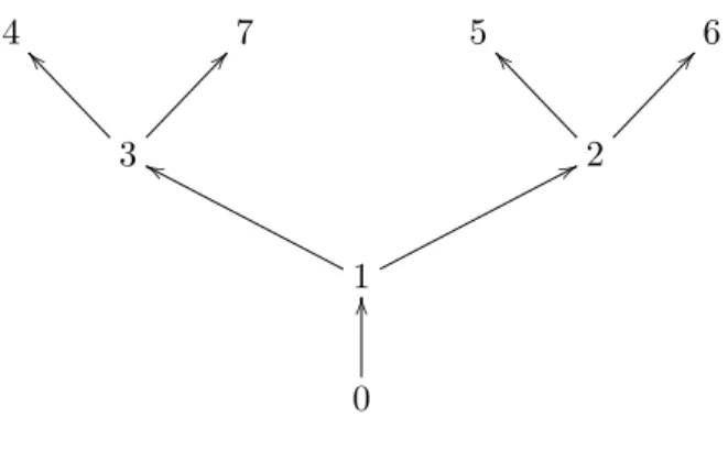
Example 5.1 This example illustrates tree structure. Let T = {0,1, . . . ,7}, and consider the following diagram, illustrating the graph G∗:
4 7 5 6
3
^^ @@
2
^^ @@
1
gg 77
0
OO
Figure 1: A Tree
Edge (s, t) ∈ E0 (the edge set for the monotone incentive graph) if in Figure 1 there is a directed path from s to t. For example, the arrow from 3 to 4 means that 4 can mimic 3 and the path
1 → 3 → 4 means that 4 can mimic 1. Let the numbers of the types also represent their values. As usual π0 = 0. Suppose that π1 = π2 = π3 =: πa and π4 = π5 = π6 = π7 =: πb. If πb/πa is
sufficiently small, then the unique optimal mechanism sells the object to all types except 0 and 1, sets a price of 2 for types 2, 5, and 6, and a price of 3 for types 3, 4, and 7. In contrast, if πb/πais
sufficiently large, only types 4, 5, 6, and 7 are served, and each is charged a price equal to her value. As stated by Proposition 5.3, in both cases, the optimal mechanism is deterministic. However, the optimal mechanism does involve price discrimination as different types receive different prices.
In light of Propostion 5.3, it is instructive to reconsider the student ID example (Example 4.1).
When only students have an ID, the optimal mechanism was randomized. Let HS and LS stand
for the high and low value students respectively and N S stand for the non-students. Then the graphG∗ is given by:
HS
N S
<<
LS
bb
0
bb <<
Figure 2: G∗ for Student ID Example
AlthoughLS can mimicN S, there is no edge from LS toN S because non-students have a higher value than low value students and G∗ does not contain bad edges. As there are two paths from 0 toHS,G∗ is not a tree.
Proposition 5.4 (Allocation monotonicity) If G∗ is a tree, then every optimal mechanism
(q, p) is monotone in the sense that if (s, t) is a good edge inE, then qs≤qt.
Proof. In Appendix.
This strengthens the form of allocation monotonicity of part 2 of Proposition 5.2, and approaches the form of allocation monotonicity present in the standard monopoly problem.17
Tree structure depends on the assignment of values to types. Next we provide a characteri-zation of the incentive graphs which induce a deterministic optimum independently of the value assignment.
Let V◦ be the set of vertices with outdegree zero in G, so that V◦ represents the set of types that cannot be mimicked by other types. Define:
˜
V :=V \(V◦∪0), E˜ :={(s, t)∈E:s6= 0, t6∈V◦}, G˜ = ( ˜V ,E˜).
Let {Gi = (Vi, Ei) : i= 1, . . . , n} be the set of weakly connected components of ˜G. Say that G is
essentially segmented if (i) Gi is strongly connected fori = 1, . . . , n, and (ii) for each t ∈V◦,
there exists i such that {s∈ V \0 : (s, t) ∈ E} ⊆Vi. (For the definition of weakly and strongly
connected components, see Section 2.3).
Proposition 5.5 (Essential segmentation) G induces a deterministic optimum for all assign-ments of values and probabilities if and only if G is essentially segmented.
Proof. In appendix.
Essential segmentation is similar to but slightly weaker than the standard assumption associated with third degree price discrimination that the seller can distinguish between different consumer segments.18 This corresponds in our model to the situation where (nonzero) types can be partitioned into segments such that all types within a segment can mimic one another and no type in any segment can mimic any type in a different segment. This means that incentive constraints must be honored within segments but not across segments. Such an incentive graph would be induced if agents within a segment have the same evidence and the evidence of any one segment is not a subset of the evidence of any other segment. Essential segmentation is weaker than standard segmentation only insofar as it allows for types t with outdegree zero (i.e., types who cannot be mimicked by any other types), such that t can mimic types in at most one segment. When there are no such zero outdegree types–that is when V◦ = ∅–then essential segmentation reduces to the standard notion of segmentation. As under essential segmentation, each type can claim mimic types in only one segment, we can interpret Proposition 5.5 to mean that transparency of segments is very close to a necessary and sufficient condition for third degree price discrimination to be always optimal (independent of the values and probabilities of types).
17
Whereas in the standard monopoly problem, allocation monotonicity follows fromfeasibility, whenG∗ is a tree, allocation monotonicity requires the stronger assumption ofoptimality. See the discussion following Proposition 5.2.
Say that valuation assignment (vt : t ∈ T) is nondegenerate if ∀s, t ∈ T, s 6= t ⇒ vs 6= vt.
Lemma 5.1 relates tree structure to essential segmentation (Propositions 5.3 and 5.5).
Lemma 5.1 G is essentially segmented if and only if for all nondegenerate values assignmentsv,
G∗v is a tree.
Proof. In appendix.
In the deterministic case, under an additional assumption, we can strengthen Proposition 5.1 to arrive at a stronger characterization of the optimum in terms of virtual values. When G∗ is a tree, define the quasi-virtual valueof type tas:
b
ψ(t) :=vt−
X
s:(t,s)∈E∗
(vs−vt)
Πs
πt
, (23)
where
Πs:=πs+
X
r:(s,r)∈E0
πr. (24)
Observe that Πs is defined with respect to the edge set E0 in the monotone incentive graph and
b
ψ(t) is defined with respect to the edge setE∗ of the transitive reduction.
Whereas the virtual value as defined by (20) is endogenous, in that it depends on an optimal solution to the dual of the seller’s problem, the quasi-virtual value defined by (23) is exogenous, defined purely in terms of primitives. Terminologically, (23) is more similar to the notion of virtual value in Myerson (1982), whereas (20) is more similar to the notions in Myerson (1991) and Myerson (2002). Because the sign of the expression in (20) is always a reliable guide to the allotment of the object, whereas the sign of (23) is only a reliable guide to the allotment of the object under special assumptions, we call the expression in (20) the virtual value, and the expression in (23) the quasi-virtual value.
Say that quasi-virtual values aresingle-crossing if: (s, t)∈E0 ⇒ψbs ≥0⇒ψbt≥0
, ∀s, t∈V.
In the standard case of the complete incentive graph, single-crossing monotone virtual values is a weakening of the common assumption of monotone quasi-virtual values (see Section 3 and especially (10)). Under tree structure and single-crossing quasi-virtual values, we attain a strengthening of Proposition 5.1, which is also an analogue of the characterization of optimal auctions due to Myerson (1982).
Proposition 5.6 Assume thatG∗ is a tree, and that quasi-virtual values are single-crossing. Then an optimal mechanism serves each type exactly if her quasi-virtual value is nonnegative.19 Formally,
19
One could replace the term “nonnegative” by “positive”, and correspondingly replace the weak inequalities by strict inequalities in (25) and the proposition would continue to be true.
an optimal mechanism (q∗, p∗) is:
q∗t =
1, if ψb(t)≥0;
0, otherwise. , p
∗
t =
(
min
{vt} ∪ {vs : (s, t)∈E,ψb(s)≥0}
, if ψb(t)≥0;
0, otherwise. (25)
Proof. In Appendix.
Remark 5.1 Single-crossing virtual values are sufficient for Proposition 5.6 because we deal with the single agent case. In the mutli-agent case, we would need to assume monotone virtual values.
Assuming tree structure and single-crossing quasi-virtual values, Proposition 5.1 shows that the optimal mechanism can be found simply by computing the quasi-virtual values. When tree structure holds, but the assumption of single-crossing quasi-virtual values fails, then it is only slightly more difficult to find the optimal mechanism. The optimal mechanism can then be found by solving a simple perfect information game between the seller and nature by backward induction. We describe this game in Section A.3 of the appendix.
6
A Revenue Formula
Section 5 described the properties of the optimal mechanism when the incentive graph is incomplete. The analysis revealed analogies (and disanalogies) to the classical analysis. Specifically, an analog of the classical notion of virtual value plays a prominent role in our analysis. This section explores a another related analogy between classical mechanism design and mechanism design with an incomplete incentive graph: revenue equivalence.
In classical mechanism design, when types are continuous, the allocation determines the revenue (up to a constant). Even in the classical case with complete incentive graph, when types are discrete as in Section 3, we do not attain exact revenue equivalence, but we do attain a formula for expressing themaximal revenue consistent with an allocation in terms of that allocation, which is analogous to the formula for expressing the unique revenue in terms of the allocation in the continuous case. In this section, we derive an analog of the classical discrete revenue formula when the incentive graph is incomplete. In addition to its intrinsic interest, Proposition 6.2 served as a useful lemma for proving several of the results in previous sections.
Primal Problem (Paths)
maximize
(qt,pt)t∈T
X
t∈T
πtpt (26)
subject to
∀(t0, t1, . . . , tk)∈ P, ptk ≤vtkqtk−
k−1
X
r=1
qtr(vtr+1−vtr)−vt1qt0 (27)
∀t∈T, 0≤qt≤1 (28)
p0= 0 (29)
We call this the path formulation, as opposed to the edge formulation (4-7), because whereas the edge formulation contained an incentive constraint for every edge in the incentive graph, the path formulation contains a related constraint for every path in the the incentive graph.20 The path formulation is a relaxation of the edge formulation but the following proposition shows that the two are equivalent for our purposes.
Proposition 6.1 The path and edge formulations of the primal have the same set of optima.
Proof. In Appendix.
It follows that:
Proposition 6.2 (Discrete Revenue Formula) Given any incentive compatible allocation q, the revenue maximizing prices that implement that allocation are:
pt= max P=(t0,...,tnP)∈Pt
vtnPqtnP − nP−1
X
i=1
qti(vti+1−vti)−vt1qt0 (30)
A path P solving the maximization (30) will always bind at the revenue maximizing prices imple-menting q.
Proposition 6.2 is a corollary of Proposition 6.1 because it follows by setting each priceptequal to the
lowest upper bound determined by (27) in the path formulation of the primal. This result generalizes the revenue formula in part 2 of Proposition 3.1. That formula does not contain a maximization because we knowa priori that the downward adjacent constraints are binding. Similarly, whenG∗
20
The constraints (27) can be interpreted in terms of path lengths: Given an allocationq= (qt :t∈T), for each
edge (s, t)∈E, interpretvt(qt−qs) as the “length” of the edge. Given any patht0 →t1→ · · · →tkinG, the induced
path length is the sum of its edge lengthsPk
j=1vtj(qtj−qtj−1). Regrouping terms, (27) can then be interpreted as
is a tree there is a unique 0−t pathP =t0 → · · · →tn=t inG∗ and for any monotone feasible
allocation (i.e., an allocation satisfying (s, t)∈E0⇒qs ≤qt),21 (6.2) simplifies to:
pt=vtnqtn−
n−1
X
i=1
qti(vti+1−vti)−vt1qt0
We conclude this section by displaying displaying the dual of (26-29), which we call the path formulation of the dual, and is an alternative to the edge formulation of the dual.
The path formulation of the dual will be useful for describing the credible implementation of the optimal mechanism in Section 7.
Dual Problem (Paths)
minimize
(µt)t∈T,(λP)P∈P
X
t∈T
µt (31)
subject to
∀t∈T\0, X
P∈Pt
λP =πt (32)
∀t∈T, vtπt−
X
s:(t,s)∈E
X
{P∈P:(t,s)∈P}
λP(vs−vt)≤µt (33)
∀P ∈ P, λP ≥0 (34)
∀t∈T, µt≥0 (35)
Dual variables indexed by edges λ(s, t) in (12-16) have been replaced by variables λP indexed by
paths in (31-35). Any feasible solution to the path formulation (λP :P ∈ P) of the dual induces
a feasible solution to the edge formulation (12-16) – for the same vector (µt : t ∈ T) – via the
relation:22
λ(s, t) = X
P3(s,t)
λP, ∀(s, t)∈E, (36)
21
In the case of the complete incentive graph, we did not need to specify that (11) was monotone over and above being feasible (i.e., incentive compatible,) because with the complete incentive graph every incentive compatible allocation is monotone.
22To see why (λ(s, t) : (s, t)∈E) defined by (36) is feasible in the edge formulation of the dual (given the fixed vector µ), note first that (36) and the fact that (µ,(λP :P ∈ P)) satisfy (33) immediately imply that (µ, λ(s, t) : (s, t)∈E)
satisfies (14). Moreover, (32) and (36) imply:
X
s:(s,t)∈E
λ(s, t)− X
s:(t,s)∈E
λ(t, s) = X
s:(s,t)∈E
X
P3(s,t)
λP −
X
s:(t,s)∈E
X
P3(t,s)
λP =
X
P3t
λP−
X
P3t:P6∈Pt
λP =
X
P∈Pt
λP =πt
where the summation on the right hand side of (36) is over paths in P containing the edge (s, t). Say thatλ= (λP :P ∈ P) isgoodif the corresponding vector (λ(s, t) : (s, t)∈E) defined by (36)
is good (see (22)). λis said to beproportionalif
∀P = (t0, . . . , tn)∈ P, λP =
" n Y
i=1
P
P03(t
i−1,ti)λP0
P
P03t
iλP0
#
πtn (37)
Under the network flow interpretation mentioned above,23 λP can be interpreted as a flow on
paths, λ(s, t) can be interpreted as a flow on edges, and the property of proportionality (37) can be interpreted as factoring the flow on paths into a (normalized) product of flows on edges. The following result will be useful for our credibility result in Section 7.
Proposition 6.3 Let µ= (µt :t ∈T) and λ= (λ(s, t) : (s, t) ∈E). Suppose (λ, µ) is optimal in
the edge formulation of the dual, and λ is good. (An optimal solution that is also good exists by part 1 of Proposition 5.2). Then there exists a unique proportional vector ˜λ= (λP :P ∈ P)related
to λby (36). Moreover (˜λ, µ) is optimal in the path formulation of the dual.
Proof. In Appendix.
In light of Proposition 6.3, when discussing a good optimal solution (µ,(λ(s, t) : (s, t) ∈ E)), we freely interchange (λ(s, t) : (s, t) ∈ E) with (λP : P ∈ P), where the latter is the unique
proportional vector corresponding to the former via (36).
7
A Credibility Result
7.1 Motivation
This section considers how the optimal mechanism might be implemented. Consider first a naive approach. The seller requests that the buyer present a cheap talk message about his type along with evidence. The seller claims, without commitment, that if the buyer submits cheap talk claim
tand evidenceSt, the seller will offer to sell the object with probabilityqt for an expected price of
pt.24 (The precise details of whether payment is made prior to the randomization or conditional on
receipt of the object can be spelled out in various ways). A problem with this approach is that if the buyer always reported truthfully, the seller would know the buyer’s value, and so would often prefer to charge a higher price, and moreover to sell the object with probability one regardless of the allocationqt.
There are many alternatives to the naive approach, whose plausibility would depend on, among other things, the seller’s commitment power. Here we pursue a particularly simple and natural
23
See Ahuja, Magnanti, and Orlin (1993) for a comprehensive treatment of network flows.
24Assume that if the evidence submitted is not the maximum evidence of the typetin the cheap talk claim, the buyer neither receives the object nor makes a payment.
approach based on minimal commitment power. We introduce a simple bargaining protocol with back-and-forth communication in which the seller can commit to honoring a take-it-or-leave-it offer once she has made it. The seller cannot commit to making any specific offer in the future contingent on various events, such as presentation of evidence. She can only commit to honoring an offer for sale with probability one and not to any form of randomization. Our bargaining protocol implements the optimal mechanism as a sequential equilibrium.
In effect, what we have done is to reduce the entire commitment problem – the commitment to a complex randomized mechanism requiring price discrimination on the basis of evidence – to the commitment to a take-it-or-leave-it offer. Any foundation for this latter simpler commitment has a potential to serve as a foundation for commitment to our more complex mechanism as well.25 Our bargaining model applies best in settings where the seller deals directly with the buyer and has the discretion to lower prices. This is the case in many firms that employ sales agents who are permitted, at their discretion, to offer discounts off the list price.26 It may not be appropriate for settings where interaction is more anonymous and distant.
One virtue of our bargaining protocol is that it has a closer resemblance to real-world negotiation than the direct mechanism. Specifically, a random allocation is generated not by commitment to randomize in response to certain messages and evidence, but rather arises naturally out of the randomized equilibrium strategies that can lead negotiations to break down. Another virtue of our protocol is that it provides an appealing interpretation of the dual of the seller’s revenue-maximization problem: At an optimal solution, the dual variables can be interpreted as encoding the buyer’s reporting strategy in the bargaining protocol.
7.2 The Bargaining Game
We now describe our bargaining game:
25
For example, Ausubel and Deneckere (1989) provide a foundation for seller commitment to take-it-or-leave-it offers in terms of the equilibrium of an infinite horizon bargaining game. However, further analysis would be required to integrate their approach to founding commitment to take-it-or-leave-it offers on the equilibrium of a repeated interaction with our quite different approach to founding commitment to a complex randomized price discrimination mechanisms on commitment to take-it-or-leave-it offers. This is beyond the scope of the current paper. For an analysis related to Ausubel and Deneckere (1989), see also Gerardi, Horner, and Maestri (2010).
26
For example a recent survey by the consulting firm Oliver Wyman reports that discretion is allowed in approxi-mately 50% of the unsecured loans and more than 60% of the secured loans offered by major European banks (Efma, Oliver Wyman Study 2012).
Dynamic Bargaining Protocol
1. Nature selects a type t∈T for the buyer with probabilityπt.
2. The buyer either:
(a) drops out and the interaction ends, or
(b) makes a cheap talk report of ˆt(where ˆt is a type inT). 3. The seller either:
(a) requests another cheap talk message, in which case we return to step 2 (this occurs at most|T|times),
(b) or requests evidence. 4. The buyer can
(a) drop out and the interaction ends, or (b) present evidence S⊆σ(t).
5. The seller makes a take-it-or-leave-it-offer.
Note At step 3, when the seller requests a cheap talk message or evidence, the seller does not specify which cheap talk message or which evidence is to be furnished.
To summarize, the buyer opens with a cheap talk claim ˆt, which implicitly includes an offer to pay
vˆt, the value of type ˆt. The seller responds either by asking for another offer or demanding proof in
return for sale at an announced price. Note that the buyer’s cheap talk claims contain information about the evidence that she possesses as well as her value. There is no discounting, so that we think of this as a fast interaction.
7.3 Credible Implementation
We now state our main result concerning the bargaining game.
Proposition 7.1 (Credibility Result) There is a sequential equilibrium of the dynamic bargain-ing protocol that implements the optimal mechanism.27
Proof. In Appendix.
We call a sequential equilibrium implementing the optimal mechanism acredible implemen-tation. The remainder of this section describes the equilibrium of Proposition 7.1 and highlights the main qualitative features of the equilibrium.
27
If there is more than one optimal mechanism, then for every optimal mechanism, there is a sequential equilibrium of the bargaining protocol that implements it.
7.3.1 Equilibrium Strategies
We now describe the strategies in the equilibrium of Proposition 7.1. The description omits details of off-path play, which are to be found in the appendix.
It is of interest that the seller’s strategy depends on an optimal solution to the seller’s revenue maximization problem (the primal (4-7)), and the buyer’s strategy depends on an optimal solution to the dual.
The buyer’s strategy: We may assume that after her typet is realized, the buyer performs a private preliminary randomization that guides her behavior throughout the game. Specifically, the buyer randomizes over paths leading tot (i.e., those inPt), selecting pathP with probability:
λP
πt
(38) whereλis an optimal proportional and good solution of the path formulation of the dual. (For the meaning of proportionality and good, see (37) and the surrounding discussion in Section 6.) (32) implies that these probabilities sum to one. When
P : 0 =t∗0→ · · · →t∗k→ · · · →t∗n=t (39)
is the outcome of the preliminary randomization, the typetbuyer reports along path (39), so that her first cheap talk claim is t∗0(= 0), if she is asked to make akth cheap talk claim, she will report
t∗k, and so on. If evidence is requested following cheap talk reportt∗k, she presents evidence St∗k.28
She drops out if asked for more cheap talk after t∗n(=t). The buyer accepts any take-it-or-leave it offer up to her valuevt, and rejects higher offers.
The seller’s strategy: Let (qt : t ∈ T) be an allocation in an optimal solution to the seller’s
revenue maximization problem. On the equilibrium path, when the buyer has made the sequence of reports (t0, . . . , tk), the seller requests evidence with probability (qtk −qtk−1)/(1−qtk−1) and
requests another cheap talk report with the remaining probability.29 (Ifk= 0, the buyer requests another cheap talk report with probability 1.) If the buyer presentsStk in response to the seller’s
evidence request, the seller makes a take-it-or-leave-it offer at price vtk. If the seller presents any
other evidence S, the seller makes an offer at the price equal to the maximum value of any type that has access toS.
28
ThatP ∈ Ptimplies that it is feasible for the typetbuyer to present evidenceSt∗k.
29
7.3.2 Qualitative Properties of Equilibrium
Call any strategy profile in which the players’ strategies satisfy the properties specified in Section 7.3.1canonical.30 A credible implementation is canonical if the strategies it employs are canonical. The proof of Proposition 7.1 establishes the existence of a canonical credible implementation. The following propositions provide key qualitative features of canonical equilibria.
Proposition 7.2 Let (t0, t1, . . . , tk) be any sequence of cheap talk reports that occur with positive
probability in a canonical credible implementation. Then:
vt0 < vt1 <· · ·< vtn (40)
St0 ⊆St2 ⊆ · · · ⊆Stn (41)
In words, both the buyer’s claimed value and the amount of claimed evidence increase as bargaining proceeds, so the buyer makes a sequence of concessions, and brings up additional evidence without retracting her claim to possess previously mentioned evidence. Moreover, when the true type is t:
Sti ⊆σ(t), fori= 0,1, . . . , k.
The buyer never claims to possess evidence that she does not possess.
Proof. In Appendix.
Proposition 7.3 For each natural numbern, there exists an environment – a set of types, values, and probabilities, and an incentive graph – such that in any canonical credible implementation, there is a positive probability that the players communicate for at least nrounds.
Proof. In Appendix.
Proposition 7.3 relates our analysis to the literature on long cheap talk (Aumann and Hart 2003, Forges and Koessler 2008). The proof constructs a sequence of environments, one for each natural number n, such that in the nth environment, any canonical credible implementation in-volves approximatelynrounds of communication. Proposition 7.3 applies only tocanonicalcredible implementations, but we believe that it is difficult to see how one could possibly bound communica-tion in the sequence of environments constructed in the proof in some other non-canonical credible implementation. The key property generating the long communication in these environments is that the optimal mechanism contains a long chain of types linked by binding incentive constraints along which the allocation probability strictly increases. The length of these chains approaches infinity asn becomes large. If the reader is interested in a concrete illustration of how a credible implementation works, we recommend the proof of Proposition 7.3 as an illustration.
30For a strategy profile to be canonical, it is not required that it satisfies the off-path properties specified in the appendix.
7.3.3 Proof Outline
The proof of Proposition 7.1 must establish four claims:
1. The equilibrium strategies described in section 7.3.1 – if followed – will implement the optimal mechanism. That is, if (qt, pt : t ∈ T) is an optimal mechanism, these strategies will lead
buyer type t to receive the object with probabilityqt and to make an expected payment of
pt.
2. The buyer’s strategy is a best reply to the seller’s strategy. 3. The seller’s strategy is a best reply to the buyer’s strategy.
4. The off-equilibrium path requirements of sequential equilibrium are met.
The appendix establishes the first two claims and the last. Next we informally describe the argument for the seller’s best reply, which turns out to be the most interesting argument. That claim too is formally established in the appendix.
7.3.4 Optimal Stopping Interpretation of the Seller’s Equilibrium Problem
Given the buyer’s equilibrium strategy, the seller’s problem in the dynamic bargaining protocol becomes an optimal stopping problem. We argue in the appendix that the seller can restrict attention tostopping strategies, which are strategies such that:
• If the buyer made reports (t0, . . . , tk) prior to the seller’s request for evidence, and presented
evidence Stk, the seller offers price vtk.
31
Because on the equilibrium path, the buyer always presents evidenceStk if asked for evidence after
type reports (t0, . . . , tk), the seller’s problem becomes an optimal stopping problem: Following
history (t0, . . . , tk), if the seller stops, requesting evidence, he receives a payoff ofvtk. If the seller
continues, requesting more cheap talk, the buyer may drop out, yielding the seller a zero payoff. If the buyer does not drop out, presenting another cheap talk claim tk+1, the seller can secure a
payoff of vtk+1 by stopping in the following round. As mentioned in Proposition 7.2, vtk < vtk+1,
so, by waiting, the seller may attain a higher reward.
The stochastic process facing the seller in his optimal stopping problem is endogenous because it depends not only on the distribution of types, but also on the buyer’s reporting strategy. If the buyer reported (t1, . . . , tk), and then the seller continued, requesting more cheap talk, the
31Ultimately, in constructing the equilibrium, we will modify the seller’s optimal stopping strategy off the equilib-rium path to insure buyer optimization.