Decomposing a Scene into Geometric and Semantically Consistent Regions
Stephen Gould
Dept. of Electrical Engineering
Stanford University
[email protected]Richard Fulton
Dept. of Computer Science
Stanford University
[email protected]Daphne Koller
Dept. of Computer Science
Stanford University
[email protected]Abstract
High-level, or holistic, scene understanding involves reasoning about objects, regions, and the 3D relationships between them. This requires a representation above the level of pixels that can be endowed with high-level at-tributes such as class of object/region, its orientation, and (rough 3D) location within the scene. Towards this goal, we propose a region-based model which combines appearance and scene geometry to automatically decompose a scene into semantically meaningful regions. Our model is defined in terms of a unified energy function over scene appearance and structure. We show how this energy function can be learned from data and present an efficient inference tech-nique that makes use of multiple over-segmentations of the image to propose moves in the energy-space. We show, ex-perimentally, that our method achieves state-of-the-art per-formance on the tasks of both multi-class image segmen-tation and geometric reasoning. Finally, by understanding region classes and geometry, we show how our model can be used as the basis for 3D reconstruction of the scene.
1. Introduction
With recent success on many vision subtasks—object de-tection [21, 18, 3], multi-class image segmentation [17, 7, 13], and 3D reconstruction [10, 16]—holistic scene under-standing has emerged as one of the next great challenges for computer vision [11, 9, 19]. Here the aim is to reason jointly about objects, regions and geometry of a scene with the hope of avoiding the many errors induced by modeling these tasks in isolation.
An important step towards the goal of holistic scene un-derstanding is to decompose the scene into regions that are semantically labeled and placed relative to each other within a coherent scene geometry. Such an analysis gives a high-level understanding of the overall structure of the scene, al-lowing us to derive a notion of relative object scale, height above ground, and placement relative to important semantic categories such as road, grass, water, buildings or sky. We provide a novel method that addresses this goal.
Our method is based on a unified model where each pixel in the image is assigned to a single region. Regions are labeled both with a semantic category (such as grass, sky, foreground, and so on) and a geometric label (currently ver-tical, horizontal, or sky). Unlike methods that deal only with multi-class segmentation [17] or only with geometric reconstruction [10], our approach reasons jointly about both aspects of the scene, allowing us to avoid inconsistencies (such as vertical roads) and to utilize the context to reduce false positives (such as unsupported objects).
A key aspect of our approach is the use of large, dynamically-defined regions as the basic semantic unit. Most previous methods for doing this type of image de-composition use either individual pixels [17] or predefined superpixels [24, 5]. Each of these approaches has its trade-offs. The use of individual pixels makes it difficult to utilize more global cues, including both robust statistics about the appearance of larger regions, which can help average out the random variations of individual pixels, and relationships be-tween regions, which are hard to “transmit” by using local interactions at the pixel level. The use of superpixels par-tially addresses some of these concerns, but as superpixels are constructed in advance using simple procedures based on local appearance alone, their boundaries are often incon-sistent with the true segment boundaries, making an accu-rate decomposition of the image impossible. Our approach dynamically associates pixels to regions, allowing region boundaries to adjust so as to accurately capture the true ob-ject boundaries. Moreover, our regions are also much larger than superpixels, allowing us to derive global appearance properties for each region, including not only color and tex-ture, but even larger properties such as its general shape, aspect ratio, and characteristics of its boundary. These fea-tures can help capture subtle yet important cues about re-gions that improve classification accuracy. As we will see, this provides a decomposition of the scenes into objects or appearance-coherent parts of objects (such as person’s head, or a window in a building).
Reasoning in our model requires that we infer both the pixel-to-region association and the semantic and geometric
labels for the regions. We address this challenge using a hy-brid approach. For the pixel-association task, we propose a novel multiple-segmentation approach, in which different precomputed segmentations are used to propose changes to the pixel-region associations. These proposed moves take large steps in the space and hence help avoid local min-ima; however, they are evaluated relative to our global en-ergy function, ensuring that each step improves the enen-ergy. The region-labeling task is addressed using global energy-minimization methods over the region space. This step is not too expensive, since the number of regions is signif-icantly lower than the number of pixels. By performing the inference at this level, we also improve labeling accu-racy because the adjacency structure between these larger regions allows us to directly exploit correlations between them (such as the fact that ground is below sky).
The parameters of our model are entirely learned from data. In this model, we are learning to label entire segments, allowing us to exploit global, region-level characteristics. We obtain positive examples for region labels from a large training set, which we constructed using Amazon Mechan-ical Turk (AMT), at a total cost of less than $250. Negative examples are a bit trickier to acquire, as there are exponen-tially many “non-regions,” most of which are obviously bad choices. We therefore propose a novel closed-loop ing regime, where the algorithm runs inference on the train-ing images given its current model, and then uses mistakes made in the process as negative examples to retrain.
We apply our method to a challenging data set consist-ing of 715 images, most of which have fairly low resolu-tion and multiple small objects at varying scales. We show that our approach produces multi-class segmentation and surface orientation results that outperform state-of-the-art methods. In addition, we show how our output can be used as the basis for 3D scene reconstruction.
2. Background and Related Work
Our work touches on many facets of computer vision that have, in recent years, been treated as separate prob-lems. The problem of multi-class image segmentation (or labeling) has been successfully addressed by a number of works [7, 22, 17, 23, 24, 5]. The goal here is to label every pixel in the image with a single class label. Typically these algorithms construct CRFs over the pixels (or small coher-ent regions called superpixels) with local class-predictors based on pixel appearance and a pairwise smoothness term to encourage neighboring pixels to take the same label. Some novel works introduce 2D layout consistency be-tween objects [23], object shape [22], or relative location between regions [7, 5]. However, none of these works take into account 3D context and do not learn or enforce global consistency, such as that “sky” needs to be above “ground”. As an alternative to segmenting into semantic classes,
Hoiem et al. [12] propose segmenting free-standing objects by estimating occlusion boundaries in an image. Other works attempt to reconstruct 3D depth [16] or surface ge-ometry [10] directly from monocular images without first reasoning about occlusions. These use local color and tex-ture cues together with pairwise interactions to infer scene structure. None of these works attempt to understand the semantic content of the scene and they tend to produce poor 3D reconstructions when foreground objects are present.
The use of multiple over-segmented images is not new to computer vision. Russell et al. [14], for example, use mul-tiple over-segmentations for finding objects in images, and many of the depth reconstruction methods described above (e.g., [10]) make use of over-segmentations for comput-ing feature statistics. In the context of multi-class image segmentation, Kohli et al. [13] specify a global objective which rewards solutions in which an entire segment is la-beled consistently. However, their energy function is very restricted and does not, for example, capture the interac-tion between region appearance and class label nor does their energy function allow for label-dependent pairwise preferences, such as foreground objects above road. Un-like all of these methods, our method uses multiple over-segmentations to build a dictionary of proposal moves for optimizing a global energy function—the segments them-selves are not used for computing features nor do they ap-pear explicitly in our objective.
The importance of holistic scene interpretation has been highlighted in a number of recent works [11, 9]. These methods combine tasks by passing the output of one model to the input of another. Unlike these approaches, which op-timize variables for each task separately, our method con-siders semantic and geometric tasks simultaneously and performs joint optimization on a unified objective over the variables, providing a coherent decomposition of the scene. Perhaps most relevant is the work of Tu et al. [20], which decomposes a scene into regions, text and faces using an innovative data driven MCMC approach on a generative model of the scene. However, their work is primarily fo-cussed on identifying text and faces, and does not attempt to label “generic” regions with semantic classes, nor do they model the geometric relationship between regions.
3. Region-based Scene Decomposition
Our goal is to decompose an imageI into an unknown number (K) of geometrically and semantically consistent regions by iteratively optimizing an energy function that measures the quality of the solution at hand. We begin by describing the various entities in our model. Inference and learning are described in Section 4.
Our model reasons about both pixels and regions. Each pixel in the image p ∈ I belongs to exactly one region, which is identified by the pixel’s region-correspondence
variableRp ∈ {1, . . . , K}. Let the set of pixels in regionr
be denoted byPr={p: Rp =r}. The size of the region
(number of pixels) is then Nr = |Pr| = Pp1{Rp=r}.
Each pixel has a local appearance feature vectorαp ∈ Rn
(described in Section 3.1 below). Associated with each re-gion are: a semantic class labelSr, currently grass,
moun-tain, water, sky, road, tree, building and foreground; a ge-ometryGr, currently horizontal, vertical, and sky; and an
appearance Ar that summarizes the appearance of the
re-gion as a whole. The final component in our model is the horizon. We assume that the image was taken by a camera with horizontal axis parallel to the ground. We therefore model the location of the horizon as the row in the image corresponding to the horizonvhz∈ {1, . . . ,height(I)}.
Given an image I and model parameters θ, our uni-fied energy function scores the entire description of the scene: the pixel-to-region associations R; the region se-mantic class labelsS, geometriesG, and appearancesA; and the location of the horizonvhz:
E(R,S,G,A, vhz, K| I,θ) =
+θhorizonψhorizon(vhz) (1) +θregionP
rψ
region
r (Sr, Gr, vhz;Ar,Pr) (2)
+θpairP
rsψ
pair
rs (Sr, Gr, Ss, Gs;Ar,Pr, As,Ps) (3)
+θboundaryP
pqψ
boundary
pq (Rp, Rq;αp, αq). (4)
We now describe each of the components of our model.
3.1. Characterizing Individual Region Appearance
For each pixelpin the image, we construct a local ap-pearance descriptor vectorαpcomprised of raw image
fea-tures and discriminitively learned boosted feafea-tures. Our raw image features, which are computed in a small neighbor-hood of the pixel, are identical to the 17-dimensional color and texture features described in [17]. We augment these raw features with more processed summaries that represent the “match” between the pixel’s local neighborhood and each of the region labels. In particular, for each (individual) semantic and geometric label we learn a one-vs-all boosted classifier to predict the label given the raw image features in a small neighborhood around the pixel.1 We then append the score (log-odds ratio) from each boosted classifier to our pixel appearance feature vectorαp.
In our experiments, we set the region appearance Arto
be the maximum-likelihood Gaussian parameters over the appearance of pixels within the region: Ar = µAr,ΣAr
where µA
r ∈ Rn andΣAr ∈ Rn×n are the mean and
co-variance matrix for the appearance vectors αpof pixels in 1In our experiments we append to the pixel’s 17 features, the average
and variance for each feature over a5×5-pixel window in 9 grid locations
around the pixel and the image row to give a total of 324 features. We use the GentleBoost algorithm with 2-split decision stumps and train for 500 rounds. Our results appeared robust to the choice of parameters.
the r-th region. These summary statistics give us a more robust estimator of the appearance of the region than would be obtained by considering only small neighborhoods of the individual pixels.
3.2. Individual Region Potentials
To define the potentials that help infer the label of indi-vidual regions, we extract features φr(Ar,Pr) ∈ Rn
de-scribing the region appearance and basic shape. Our ap-pearance features include the mean and covarianceµA
r,ΣAr,
the log-determinant ofΣA
r, and the average contrast at the
region boundary and region interior. In addition to relating to semantic class—grass is green—the appearance features provide a measure for the quality of a region—well-formed regions will tend to have strong boundary contrast and (de-pending on the class) little variation of interior appearance. We also want to capture more global characteristics of our larger regions. For example, we would like to capture the fact that buildings tend to be vertical with many straight lines, trees tend to be green and textured, and grass tends to be green and horizontal. Thus, we incorporate shape fea-tures that include normalized region area, perimeter, first and secondx- andy-moments, and residual to a robust line fit along the top and bottom boundary of the region. The latter features capture the fact that buildings tend to have straight boundaries while trees tend to be rough.
We also include the horizon variable in the region-specific potential, allowing us to include features that mea-sure the ratio of pixels in the region above and below the horizon. These features give us a sense of the scale of the object and its global position in the scene. For example, buildings are tall and tend to have more mass above the hori-zon than below it; foreground objects are often close and will have most of their mass below the horizon. Conversely, these potentials also allow us to capture the strong posi-tional correlation between the horizon and semantic classes such as sky or ground, allowing us to use the same potential to place the horizon within the image.
To put all of these features together, we learn a multi-class logistic multi-classifier forSr×Grwith a quadratic kernel
overφr(see Section 4.2). The score for any assignment to
the region variables is then: ψrregion(Sr, Gr, vhz;Ar,Pr) =
−Nrlogσ Sr×Gr|φr(Ar,Pr), vhz, whereσ(·) is the
multi-class logistic function with learned parameters. We scale the potential by the region sizeNr so that our score
gives more weight to larger regions and is independent of the number of regions in the image.
3.3. Inter-Region Potentials
Our model contains two types of inter-region poten-tials. The first of these isψpqboundary(Rp, Rq;αp, αq), which
is the standard contrast-dependent pairwise boundary po-tential [17]. For two adjacent pixels p and q, we
de-fine ψboundarypq (Rp, Rq;αp, αq) = exp{−β−1kαp −αqk2}
ifRp 6= Rq and zero otherwise whereβ is half the
aver-age contrast between all adjacent pixels in the imaver-age. This term penalizes adjacent regions that do not have an edge between them; it has the effect of trying to merge adjacent regions that are not clearly demarcated. We note that, since the penalty is accumulated over pairs of adjacent pixels, the region-level penalty is proportional to the pixel-length of the boundary between the regions.
Our second inter-region potential,ψpair, models the affin-ity of two classes to appear adjacent to each other. Sim-ilar to the within-region potentials, we extract features
φrs(Ar,Pr, As,Ps) ∈ Rm for every pair of adjacent
re-gionsrands. We then learn independent multi-class logis-tic classifiers forSr×SsandGr×Gsgiven these features.
Note that these potentials are asymmetric (exchanging re-gions r ands gives a different preference). The features
φrsare intended to model contextual properties between
re-gions, for example, the boundary between building and sky tends to be straight and building is more likely to appear above a foreground object than below it. To capture these properties, our features include the difference between cen-troids of the two regions, the proportion of pixels along the boundary in which regionris above regions, the length and orientation of the boundary, and residual in fitting a straight line to the boundary. In addition to these layout-based fea-tures, we include appearance difference between the regions normalized by the total appearance variance within each re-gion. This captures signals such as foreground objects tend to contrast highly with other regions, whereas background regions are more similar in appearance, such as adjacent buildings in a city.
We normalize each pairwise potential by the sum of the number of pixels in each region divided by the num-ber of neighbors for the region: η = Nr
|nbrs(r)|+
Ns
|nbrs(s)|
. This makes the total influence on a region independent of its number of neighbors while still giving larger regions more weight. The final form of our second inter-region potential is then ψpairrs(Sr, Gr, Ss, Gs;Ar,Pr, As,Ps) =
−ηlogσ(Sr×Ss|φrs)−ηlogσ(Gr×Gs|φrs), where,
as above,σ(·)is the multi-class logistic function.
4. Inference and Learning
4.1. Inference Algorithm
Exact inference in our model is clearly intractable. We adopt a two-stage hill climbing approach to minimize the energy. In the first stage, we modify the pixel-region asso-ciation variables by allowing a set of pixels to change the region to which they are assigned. Given the new pixel as-signments, we then optimize the region and horizon vari-ables in the second stage. The global energy of the resulting configuration is then evaluated, and the move is accepted
Procedure InferSceneDecomposition Generate over-segmentation dictionaryΩ InitializeRpusing one of the over-segmentations
Repeat until convergence
Propose a move{Rp:p∈ω} ←r
Update region appearanceAand featuresφ
Run inference over regions(S,G)and horizonvhz
Compute total total energyE
If(E < Emin)then
Accept move and setEmin=E
Else reject move
(a) (b)
Figure 1. (a) Scene decomposition inference algorithm; (b) Over-segmentation dictionary,Ω, generated by running mean-shift [1] with three different parameter settings. See text for details.
only if this energy improves, ensuring that our inference is continuously improving a coherent global objective.
The proposal moves for region associations are drawn from a pre-computed, image-specific dictionary of image segmentsΩ(Figure 1(b)). To build a “good” set of segments we start with a number of different over-segmentations of the image. Here, we use the mean-shift algorithm [1] us-ing publicly available code.2 We generate different over-segmentations by varying the spatial and range bandwidth parameters. To allow coarse granularity moves, we also perform hierarchical agglomerative clustering (up to a fixed depth) on each over-segmentation by merging adjacent seg-ments that have similar appearance. We then add all subsets constructed by this process (including the initial segments) to the dictionary. This procedure produces a rich set of pro-posal moves. We sort the dictionary by the entropy of pixel appearance within each segment so that more uniform seg-ments are proposed first.
In addition to moves proposed by the dictionary, we also allow moves in which two adjacent regions are merged to-gether. The set of allowed pixel-to-region correspondence proposal moves is thus: (i) pick a segmentω ∈ Ωand as-sign allRpforp∈ ωto a new region; (ii) pick a segment
ω ∈ Ωand assign allRp for p∈ ωto one of the regions
in its neighborhood; or (iii) pick two neighboring regionsr
andsand merge them, that is,∀Rp=ssetRp=r.
Our overall inference algorithm is summarized in Fig-ure 1(a): Briefly, we initialize our pixel-to-region associa-tions Rusing one of the over-segmentations used to pro-duce our dictionary. Given our current association R, we select a proposal move and reassign pixels to form new re-gions. We then update the appearance modelAr and
fea-tures of any region that was affected by the move. We maintain sufficient statistics over pixel appearance, making this step very fast. Keeping the pixel-to-region correspon-dence variables and horizon fixed, we run max-product be-lief propagation on the region class and geometry variables.
2http://www.caip.rutgers.edu/riul/research/ code/EDISON/index.html
We then update the horizonvhzusing Iterated Conditional Modes (ICM).3The new configuration is evaluated relative to our global energy function, and kept if it provides an im-provement. The algorithm iterates until convergence. In our experiments (Section 5) inference took between 30 seconds and 10 minutes to converge depending on image complexity (i.e., number of segments inΩ).
4.2. Learning Algorithm
We train our model using a labeled dataset where each image is segmented into regions that are semantically and geometrically coherent. Thus, our ground truth specifies both the region association for each pixel and the labels for each region.
We learn each term ψhorizon,ψregion andψpair in our en-ergy function separately, using our labeled training data. We then cross-validate the weights between the terms using a subset of our training data. Since only the relative weight-ing between terms matter, we fixedθregionto one.
For the horizon singleton term, we learn a Gaussian over the location of the horizon in training images and set
ψhorizon(vhz)to be the log-likelihood ofvhzgiven this model. We normalize ψhorizon(vhz) by the image height to make this model resolution invariant. Our learned Gaussian has a mean of approximately 0.5 and standard deviation of 0.15 (varying slightly across experiment folds). This suggests that the horizon in our dataset is quite well spread around the center of the image.
The within-region term,ψregion, and the between-region term,ψpair, are learned using multi-class logistic regression. However, the training of the within-region term involves an important subtlety. One of the main roles of this term is to help recognize when a given collection of pixels is actually a coherent region—one corresponding to a single semantic class and a single geometry. Although all of the regions in our training set are coherent, many of the moves proposed during the course of inference are not. For example, our algorithm may propose a move that merges together pixels containing (horizontal) grass and pixels containing (verti-cal) trees. We want to train our classifier to recognize in-valid moves and penalize them. To penalize such moves, we train our multi-class logistic regression classifier with an additional “invalid” label. This label cannot be assigned to a candidate region during inference, and so if the pro-posed regionrappears incoherent, the “invalid” label will get high probability, reducing the probability for all (valid) labels inSr×Gr. This induces a high energy for the new
proposed assignment, making it likely to be rejected. To train a discriminative classifier that distinguishes
be-3We experimented with includingvhzin the belief propagation infer-ence but found that it changed very little from one iteration to the next and was therefore more efficient to infer conditionally (using ICM) once the other variables were assigned.
tween coherent and incoherent regions, we need to provide it with negative (incoherent) training instances. Here, we cannot simply collect arbitrary subsets of adjacent pixels that do not correspond to coherent regions: Most arbitrary subsets of pixels are easily seen to be incoherent, so that a discriminative model trained with such subsets as negative examples is unlikely to learn a meaningful decision bound-ary. Therefore, we use a novel “closed-loop” learning pro-cedure, where the algorithm trains on its own mistakes. We begin by training our classifier where the negative exam-ples are defined by merging pairs of adjacent ground truth regions (which are not consistent with each other). We then perform inference (on our training set) using this model. During each proposal move we evaluate the outcome of in-ference with the ground truth annotations. We append to our training set moves that were incorrectly accepted or re-jected, or moves that were accepted (resulted in lower en-ergy) but produced an incorrect labeling of the region vari-ables. In this way, we can target the training of our decision boundary on the more troublesome examples.
5. Experimental Results
We conduct experiments on a set of 715 images of ur-ban and rural scenes assembled from a collection of public image datasets: LabelMe [15], MSRC [2], PASCAL [4], and Geometric Context (GC) [10]. Our selection criteria were for the images to have approximately320×240 pix-els, contain at least one foreground object and have the hori-zon positioned within the image (it need not be visible). We perform 5-fold cross-validation with the dataset randomly split into 572 training images and 143 test images for each fold. The quality of our annotations (obtained from Ama-zon Mechanical Turk) is extremely good and in many cases superior to those provided by the original datasets. Images and labels are available for download from the first author’s website.
Baselines. To validate our method and provide strong baselines for comparison, we performed experiments on independent multi-class image segmentation and geometry prediction using standard pixelwise CRF models. Here the pixel classSp (or surface geometryGp) is predicted
sepa-rately for each pixelp∈ Igiven the pixel’s appearanceαp
(see Section 3.1). A contrast-dependent pairwise smooth-ness term is added to encourage adjacent pixels to take the same value. The models have the form
E(S| I) =X
p
ψp(Sp;αp) +θ
X
pq
ψpq(Sp, Sq;αp, αq)
and similarly forE(G| I). In this model, each pixel can be thought of as belonging to its own region. The parameters are learned as described above withψpa multi-class
logis-tic over boosted appearance features andψpqthe boundary
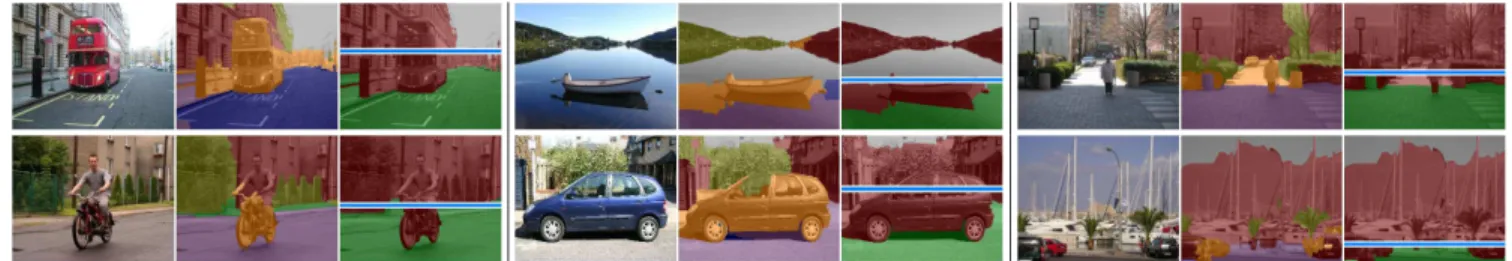
Figure 2. Examples of typical scene decompositions produced by our method. Show for each image are regions (top right), seman-tic class overlay (bottom left), and surface geometry with horizon (bottom right). Best viewed in color.
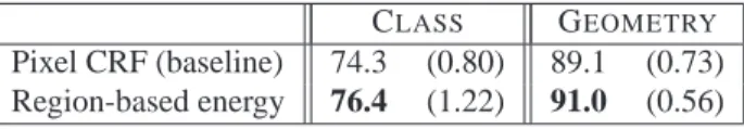
Region-based Approach. Multi-class image segmenta-tion and surface orientasegmenta-tion results from our region-based approach are shown below the baseline results in Table 1. Our improvement of 2.1% over baseline for multi-class seg-mentation and 1.9% for surface orientation is significant. In particular, we observed an improvement in each of our five folds. Our horizon prediction was within an average of 6.9% (relative to image height) of the true horizon.
In order to evaluate the quality of our decomposition, we computed the overlap score between our boundary predic-tions and our hand annotated boundaries. To make this met-ric robust we first dilate both the predicted and ground truth boundaries by five pixels. We then compute the overlap score by dividing the total number of overlapping pixels by half the total number of (dilated) boundary pixels (ground truth and predicted). A score of one indicates perfect over-lap. We averaged 0.499 across the five folds indicating that on average we get about half of the semantic boundaries correct. For comparison, using the baseline class predic-tions gives a boundary overlap score of 0.454.
The boundary score result reflects our algorithm’s ten-dency to break regions into multiple segments. For exam-ple, it tends to leave windows separated from buildings and people’s torsos separated from their legs (as can be seen in Figure 2). This is not surprising given the strong appearance difference between these different parts. We hope to extend our model in the future with object specific appearance and shape models so that we can avoid these types of errors.
Figures 3 and 4 show some good and bad examples, re-spectively. Notice the high quality of the class and geome-try predictions particularly at the boundary between classes and how our algorithm deals well with both near and far ob-jects. There are still many mistakes that we would like to
CLASS GEOMETRY Pixel CRF (baseline) 74.3 (0.80) 89.1 (0.73) Region-based energy 76.4 (1.22) 91.0 (0.56) Table 1. Multi-class image segmentation and surface orientation (geometry) accuracy. Standard deviation shown in parentheses.
MSRC GC
TextonBoost [17] 72.2 Hoiem et al. [10]: Yang et al. [24] 75.1 •pixel model 82.1 Gould et al. [5] 76.5 •full model 88.1 Pixel CRF 75.3 Pixel CRF 86.5 Region-based 76.4 Region-based 86.9 Table 2. Comparison with state-of-the-art MSRC and GC results against our restricted model. Table shows mean pixel accuracy. address in future work. For example, our algorithm is often confused by strong shadows and reflections in water as can be seen in some of the examples in Figure 4. We hope that with stronger geometric reasoning we can avoid this prob-lem. Also, without knowledge of foreground subclasses, our algorithm sometimes merges a person with a building or confuses boat masts with buildings.
Comparison with Other Methods. We also compared our method with state-of-the-art techniques on the 21-class MSRC [2] and 3-class GC [10] datasets. To make our results directly comparable with published works, we re-moved components from our model not available in the ground-truth labels for the respective datasets. That is, for MSRC we only use semantic class labels and for GC we only use (main) geometry labels. Neither model used horizon information. Despite these restrictions, our region-based energy approach is still competitive with state-of-the-art. Results are shown in Table 2.
6. Application to 3D Reconstruction
The output of our model can be used to generate novel 3D views of the scene. Our approach is very simple and ob-tains its power from our region-based decomposition rather than sophisticated features tuned for the task. Nevertheless, the results from our approach are surprisingly good com-pared to the state-of-the-art (see Figure 5 for some exam-ples). Since our model does not provide true depth estimates our goal here is to produce planar geometric reconstructions of each region with accurate relative distances rather than absolute distance. Given an estimate of the distance be-tween any two points in the scene, our 3D reconstruction can then be scaled to the appropriate size.
Our rules for reconstruction are simple. Briefly, we as-sume an ideal camera model with horizontal (x) axis paral-lel to the ground. We fix the camera origin at 1.8m above the ground (i.e.,y= 1.8). We then estimate theyz-rotation of the camera from the location of the horizon (assumed to be at depth∞) asθ= tan−1(1
f(v
hz−v0))wherev 0is half
Figure 3. Representative results when our model does well. Each cell shows original image (left), overlay of semantic class label (center), and surface geometry (right) for each image. Predicted location of horizon is shown on the geometry image. Best viewed in color.
Figure 4. Examples of where our algorithm makes mistakes, such as mislabeling of road as water (top left), or confusing boat masts as buildings (bottom right). We also have difficulty with shadows and reflections. Best viewed in color.
the image height andf is the focal length of the camera. Now the 3D location of every pixel p = (u, v)lies along the rayrp = R(θ)−1K−1[u v1]T
, whereR(θ)is the ro-tation matrix andKis the camera model [6]. It remains to scale this ray appropriately.
We process each region in the image depending on its se-mantic class. For ground plane regions (road, grass and wa-ter) we scale the ray to make the height zero. We model each vertical region (tree, building, mountain and foreground) as a planar surface whose orientation and depth with respect to the camera are estimated by fitting a robust line over the pixels along its boundary with the ground plane. This produced good results despite the fact that not all of these pixels are actually adjacent to the ground in 3D (such as the belly of the cow in Figure 5). When a region does not touch the ground (that is, it is occluded by another object), we estimate its orientation using pixels on its bottom-most
boundary. We then place the region half way between the depth of the occluding object and maximum possible depth (either the horizon or the point at which the ground plane would become visible beyond the occluding object). The 3D location of each pixelpin the region is determined by the intersection of this plane and the ray rp. Finally, sky regions are placed behind the last vertical region.4
7. Discussion and Future Work
In this work, we addressed the problem of decompos-ing a scene into geometrically and semantically coherent regions. Our method combines reasoning over both pixels and regions through a unified energy function. We proposed
4Technically, sky regions should be placed at the horizon, but since the
horizon has infinite depth, we choose to render sky regions closer, so as to make them visible in our viewer.
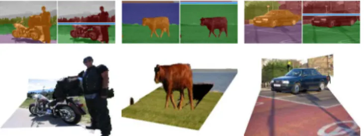
Figure 5. Novel views of a scene with foreground objects gener-ated by geometric reconstruction.
an effective inference technique for optimizing this energy function and showed how it could be learned from data. Our results compete with state-of-the-art multi-class image seg-mentation and geometric reasoning techniques. In addition, we showed how a region-based approach can be applied to the task of 3D reconstruction, with promising results.
Our framework provides a basis on which many valu-able extensions can be layered. With respect to 3D recon-struction, our method achieves surprising success given that it uses only simple geometric reasoning derived from the scene decomposition and location of the horizon. These results could undoubtedly be improved further by integrat-ing our method with state-of-the-art approaches that reason more explicitly about depth [16] or occlusion [12].
An important and natural extension to our method can be provided by incorporating object-based reasoning directly into our model. Here, we can simply refine our foreground class into subclasses representing object categories (person, car, cow, boat, etc.). Such models would allow us to incor-porate information regarding the relative location of differ-ent classes (cars are found on roads), which are very natu-rally expressed in a framework that explicitly models large regions and their (rough) relative location in 3D. By reason-ing about different object classes, we can also incorporate state-of-the-art models regarding object shape [8] and ap-pearance features [3]. We believe that this extension would allow us to address one of the important error modes of our algorithm, whereby foreground objects are often broken up into subregions that have different local appearance (a per-son’s head, torso, and legs). Thus, this approach might al-low us to decompose the foreground class into regions that correspond to semantically coherent objects (such as indi-vidual people or cars).
Finally, an important limitation of our current approach is its reliance on a large amount of hand-labeled training data. We hope to extend our framework to make use of large corpora of partially labeled data, or perhaps by using motion cues in videos to derive segmentation labels.
Acknowledgments. We give warm thanks to Geremy Heitz and
Ben Packer for the many helpful discussions regarding this work. This work was supported by DARPA T/L SA4996-10929-4 and MURI contract N000140710747.
References
[1] D. Comaniciu, P. Meer, and S. Member. Mean shift: A robust approach toward feature space analysis. PAMI, 2002. [2] A. Criminisi. Microsoft research cambridge object
recog-nition image database. http://research.microsoft.com/vis-ion/cambridge/recognition, 2004.
[3] N. Dalal and B. Triggs. Histograms of oriented gradients for human detection. In CVPR, 2005.
[4] M. Everingham, L. Van Gool, C. K. I. Williams, J. Winn, and A. Zisserman. The PASCAL Visual Object Classes Chal-lenge 2007 (VOC2007) Results, 2007.
[5] S. Gould, J. Rodgers, D. Cohen, G. Elidan, and D. Koller. Multi-class segmentation with relative location prior. IJCV, 2008.
[6] R. I. Hartley and A. Zisserman. Multiple View Geometry in
Computer Vision. Cambridge University Press, 2004.
[7] X. He, R. Zemel, and M. Carreira-Perpinan. Multiscale CRFs for image labeling. In CVPR, 2004.
[8] G. Heitz, G. Elidan, B. Packer, and D. Koller. Shape-based object localization for descriptive classification. In NIPS, 2008.
[9] G. Heitz, S. Gould, A. Saxena, and D. Koller. Cascaded classification models: Combining models for holistic scene understanding. In NIPS, 2008.
[10] D. Hoiem, A. A. Efros, and M. Hebert. Recovering surface layout from an image. IJCV, 2007.
[11] D. Hoiem, A. A. Efros, and M. Hebert. Closing the loop on scene interpretation. CVPR, 2008.
[12] D. Hoiem, A. N. Stein, A. A. Efros, and M. Hebert. Recov-ering occlusion boundaries. ICCV, 2007.
[13] P. Kohli, L. Ladicky, and P. Torr. Robust higher order poten-tials for enforcing label consistency. In CVPR, 08.
[14] B. C. Russell, A. A. Efros, J. Sivic, W. T. Freeman, and A. Zisserman. Using multiple segmentations to discover ob-jects and their extent in image collections. In CVPR, 06. [15] B. C. Russell, A. B. Torralba, K. P. Murphy, and W. T.
Free-man. Labelme: A database and web-based tool for image annotation. IJCV, 2008.
[16] A. Saxena, M. Sun, and A. Y. Ng. Learning 3-D scene struc-ture from a single still image. In PAMI, 2008.
[17] J. Shotton, J. Winn, C. Rother, and A. Criminisi. Texton-Boost: Joint appearance, shape and context modeling for multi-class obj. rec. and seg. In ECCV, 2006.
[18] A. Torralba, K. P. Murphy, and W. T. Freeman. Contextual models for object detection using BRFs. In NIPS, 2005. [19] Z. Tu. Auto-context and its application to high-level vision
tasks. In CVPR, 2008.
[20] Z. Tu, X. Chen, A. L. Yuille, and S.-C. Zhu. Image parsing: Unifying segmentation, detection, and recognition. In ICCV, 2003.
[21] P. Viola and M. J. Jones. Robust real-time face detection.
IJCV, 2004.
[22] J. Winn and N. Jojic. LOCUS: Learning object classes with unsupervised segmentation. In ICCV, 2005.
[23] J. Winn and J. Shotton. The layout consistent random field for recognizing and segmenting partially occluded objects. In CVPR, 2006.
[24] L. Yang, P. Meer, and D. J. Foran. Multiple class segmenta-tion using a unified framework over mean-shift patches. In