Two-dimensional turbulence: a physicist approach
PatrickTabeling
Laboratoire de Physique Statistique, Ecole Normale Superieure, 24 rue Lhomond, 75231 Paris, France Received June 2001; editor: I:Procaccia
Contents
1. Introduction 2
2. Exact results 4
3. Coherent structures 8
4. Statistics of the coherent structures in
decaying two-dimensional turbulence 16 5. Equilibrium states of two-dimensional
turbulence 22
6. Inverse energy cascade 29
7. Dispersion of pairs in the inverse cascade 40
8. Condensed states 42
9. Enstrophy cascade 45
10. Coherent structures vs. cascades 52
11. Conclusions 56
12. Uncited references 57
Acknowledgements 57
References 57
Abstract
Much progress has been made on two-dimensional turbulence, these last two decades, but still, a number of fundamental questions remain unanswered. The objective of the present review is to collect and organize the available information on the subject, emphasizing on aspects accessible to experiment, and outlining contributions made on simple 9ow con:gurations. Whenever possible, open questions are made explicit. Various subjects are presented: coherent structures, statistical theories, inverse cascade of energy, condensed states, Richardson law, direct cascade of enstrophy, and the inter-play between cascades and coherent structures. The review o=ers a physicist’s view on two-dimensional turbulence in the sense that experimental facts play an important role in the presentation, technical issues are described without much detail, sometimes in an oversimpli:ed form, and physical arguments are given whenever possible. I hope this bias does not jeopardize the interest of the presentation for whoever wishes to visit the fascinating world of Flatland. c 2002 Elsevier Science B.V. All rights reserved.
PACS: 47.27.Ak; 47.27.Eq; 05.45.−a
0370-1573/02/$ - see front matter c2002 Elsevier Science B.V. All rights reserved. PII: S 0370-1573(01)00064-3
1. Introduction
Several motivations or prospects may lead to get involved in studies on two-dimensional turbulence. One motivation, probably shared by all the investigators, is that hydrodynamic tur-bulence, despite its practical interest, its omnipresence, and the series of assaults it has been submitted to for decades, is still with us as the most important unsolved problem of classical mechanics. ‘Unsolved’ means that, for the simplest cases we may conceive, we are unable to infer the statistical characteristics of a turbulent system from :rst principles. It is not a matter of being unable to perform a detailed calculation. The structure of the solution is at the mo-ment beyond the reach of existing theoretical approaches. Inspiration has not lacked for devising clever theoretical methods, but for long, success did not come and in this respect, hydrodynamic turbulence looks as a cemetery for a number of ideas that turned out to be outrageously success-ful in other areas of condensed matter physics. At the moment, the situation perhaps evolves, further to recent breakthroughs made on the turbulent dispersion problem. In particular, we now have, for the passive dispersion problem, a complete knowledge of turbulent solutions for particular (idealized) cases. An issue is to what extent these ideas may be used to tackle the hydrodynamic turbulent problem. The least one can say is that the issue is open at the moment. Another motivation is related to geophysical 9ows. Flows in the atmosphere and in the ocean develop in thin rotating strati:ed layers, and it is known that rotation, strati:cation and con-:nement are eEcient vectors conveying two-dimensionality. Experimental devices developed in laboratories typically use these ingredients to prepare acceptably two-dimensional 9ows. The extent to which two-dimensional turbulence represents atmospheric or oceanographic turbulence is however not straightforward to circumvent, and this question has been discussed in several places [77,29,118]. In the simplest cases, pure two-dimensional equations must be amended by the addition of an extra-term, characterizing the e=ect of Coriolis forces, to represent physi-cally relevent situations. This term generates waves which radiate energy, a mechanism absent in pure two-dimensional systems. In more realistic cases, topography, thermodynamics, strati-:cation, must be incorporated in the analysis, and indeed full two-dimensional approximation hardly encompasses the variety of phenomena generated by these additional terms. Nonetheless, purely two-dimensional 9ows provide useful guidance to understand some important aspects of geophysical 9ows. A remarkable (although rather isolated) example is the trajectories of the tropical hurricanes. For long, two-dimensional pointwise vorticity models have been used, leading to fairly acceptable predictions. In the oceans, the concept of coherent structures, discov-ered in early studies of two-dimensional turbulent 9ows, is frequently substantiated. A context where concepts of two-dimensional turbulence appear as particularly relevant is the dispersion of chemical species in the atmosphere, and tracers in the oceans. The structure of the ozone concentration :eld around the polar vortex can be accounted for if :lamentary processes, simi-lar to those prevailing in two-dimensional turbulent 9ows, are assumed to take place. For this particular aspect, evoking the presence of waves do not provide clues while two-dimensional turbulence o=ers an interesting framework, allowing to construct acceptable representations [71]. A third motivation is linked to the three-dimensional turbulence problem. The recent period has shown the existence of a common conceptual frameworkbetween two- and three-dimensional turbulence. Phenomena, such as cascades, coherent structures, dissipative processes, :lamentation mechanisms take place in both systems. On the other hand, turbulence is simpler to represent
and easier to compute in two than in three dimensions and physical experiments provide much more information when the 9ow is thoroughly visualized that when it is probed with a sin-gle sensor. Therefore, operating in Flatland may be instructive to test ideas or theories, prior to considering them in the three-dimensional world. Note that three-dimensional turbulence is not three dimensional in all respects; an example is the worms, which populate the dissipative range: they are long tubes and thus can be tentatively viewed as to two-dimensional objects. One may also add that two-dimensional turbulence is helpful for understanding turbulence in general. Turbulence is a general phenomenon, involving nonlinear dynamics and broad range of scales, including as particular cases two- and three-dimensional 9uid turbulence, but also su-per9uid turbulence. Nonlinear ShrIodinger turbulence, scalar turbulence of any sort, i.e. passive or active, low or high Prandtl numbers, ‘burgulence’ (i.e. the particular turbulence produced in Burgers equation), to mention but a few. Across these subjects, a common conceptual framework exists, and two-dimensional turbulence can obviously be used to understand several aspects of the general problem.
If we trace backthe history, it seems that it tooka long time to realize that 9ows can be turbulent in two dimensions. For long, two-dimensional turbulence was thought impossible, frozen by too many conservation laws. Batchelor, in his in9uential textbookon turbulence [8], overlooked the possibility that turbulent cascades may exist in 2D. In the presentations of turbulence, it was not uncommon to stress that two-dimensional 9ows are inhospitable to turbulent regimes.
The situation changed in the sixties, further to two contributions, given independantly by Kraichnan and Batchelor. Batchelor reconsidered his views on two-dimensional turbulence, and proposed that cascades may develop in the plane, in a way analogous to the direct energy cascade in three dimensions, with the enstrophy playing the role of the energy [9]. Kraichnan [67] discovered the double cascade process and explained that turbulence may be compatible with the presence of several conservation laws. These contributions stimulated research in the :eld, by suggesting that something can be learnt on turbulence in general from investigations led on two-dimensional systems.
Still, the development of the :eld was considered as diEcult, since it was generally consid-ered that turbulent two-dimensional 9ows could not be achieved in the laboratory, and it was uncertain that the development of the computers could provide, within a reasonable range of time, reliable and accurate data on such systems. Now the situation has drastically changed, since on both of these aspects, we witnessed considerable developments. Numerics exploded in the seventies, and succeeded to produce a considerable 9ux of reliable data. Several phenom-ena were discovered, among them the coherent structures, which deeply modi:ed our view on turbulence. For long the available data in Flatland was computationally based; this is no more true today. The experimental e=ort, starting in the seventies with pioneering experiments, could be pushed forward, thanks to the availability of image processing techniques. In some cases, the physical experiment could o=er conclusions diEcult to draw out from numerics.
We now are in a situation where the :eld of two-dimensional turbulence has reached a sort of maturity, in the sense that numerical and experimental techniques are in position to convey valuable and relevant information concerning most of the questions we may askon the problem. This is not true as soon as complications, such as wave propagation, or topographic e=ects are added. A source of progress is certainly expected from the theory, which at the moment, is
unable to answer the simplest questions. In several cases, the theory seems to be stuck, like a bee in a honey pot, and conceptual breakthroughs appear as the only chance to move forward. Speci:c issues such as the role of coherent structures in turbulent systems, the intermittency e=ects in the inverse cancade, the ergodic issue in free systems, are example of problems which seem to raise considerable diEculties.
In this context, it seemed to me that it could be interesting to review the knowledge accumu-lated during the last decades on the subject. At the moment, the results are spread in various papers and for those who wish to get in touch with the :eld, it would take time to collect the most relevant information. Two-dimensional turbulence has already been reviewed by several authors. Kraichnan and Montgomery [69] emphasized on statistical theories, giving a complete account of the theoretical e=orts made until 1980. A more recent review on the subject, written in a pleasant pedagogical form, is given by Miller et al. [89]. Lesieur [77] reviewed di=erent subjects, emphasizing on spectral descriptions. Frisch [43] wrote a swift review, which empha-sizes many of the far-reaching issues still open in the :eld. A short account on recent progress in two-dimensional turbulence has been given by Nelkin [94]. The presentation I am propos-ing here can be viewed as an extension and an update of Frisch’s review. Some material was unavailable at that time, at theoretical, numerical and physical levels and I hope the present review will bring useful complements.
As a physicist, I will put emphasis on the experiment, and on the theoretical e=orts dedicated to explaining phenomena within the reach of the observation. This certainly tends to con:ne the view on the subject. Two-dimensional turbulence is a :eld of investigation for theorists, who need to develop their own approach without being necessarily constrained by the experimental facts. I decided to warn the reader of this personal bias by making an announcement at the :rst line of the paper, i.e. in the title. I will not make any description of closure models such as EDQNM, or test :eld model, despite their practical interest. The reader will :nd a presentation of these aspects in [77]. Also cascade models, such as shell model, will not be discussed. I hope these biases and limitations do not outrageously reduce the scope of the review, and that the present paper will be of interest for a broad range of scientists interested in turbulence, for whatever reason.
2. Exact results
There exist several exact results, important to know for understanding two-dimensional tur-bulent 9ows. They are quoted in papers by Batchelor [9], reviews by Rose and Sulem [121], Kraichnan and Montgomery [69], or books by Lesieur [77], and Frisch [43]. One starts with the Navier–Stokes equations which read:
Du
Dt =@@tu+ (u)u=−1∇p+fext+Ou; (1)
∇ ·u=0 (2)
in which u is the velocity, p the pressure, fext is the external forcing, and is the kinematic
viscosity. One usually takes a system of coordinates (x; y) for the plane of 9ow and z for the
In the inviscid case (= 0), and without forcing (fext= 0), these equations are the Euler
equations; in two dimensions, it has been possible to prove that the Euler equations are regular in a bounded domain, and, if the vorticity is initially bounded, the solution exists and is unique (see [121]). This implies in particular that there are no singularities at :nite time for the velocity, a possibility which, at the moment, is not ruled out in three dimensions.
By taking the curl of these equations, one gets an equation for the vorticity != (∇xu)z in
the form
D!
Dt =
@!
@t +u!=g+O! ; (3)
where g is the projection of the curl of the forcing, along the axis normal to the plane. Let
us stress that this equation holds in two dimensions, and not in three. In three dimensions, the governing equation for the vorticity has a di=erent form: an additional term, called vortex stretching, must be added. Sticking to the two-dimensional case, one :nds that, in the inviscid
limit (= 0), and with a curl free forcing (g= 0), the vorticity is conserved along the 9uid
particle trajectories, a result known as Helmhotz theorem. In two-dimensional inviscid 9ows, the 9uid particles keep their vorticity for ever. In three-dimensional turbulence, it is not so: the additional vortex stretching term in the vorticity equation ampli:es, in the average, vortic-ity along the trajectories, leading to the formation of small intense :laments. Freely evolving two-dimensional turbulence cannot generate small intense vortices. This di=erence, between two and three dimensions, is fundamental to underline.
A quantity of fundamental interest in turbulence is the kinetic energy per unit of mass, de:ned by
E=1
2u2 ; (4)
where the brackets mean statistical averaging, i.e. the average of a large number of independant realizations. It is usually considered that in homogeneous or spatially periodic systems, taking spatial averages is equivalent to taking statistical average. This may not be always true, but we do not address this issue in this section. In 2D, and in homogeneous or periodic systems, the evolution equation for the energy reads:
dE
dt = 12du
2
dt =−Z ; (5)
where Z=!2 is the enstrophy. This quantity is governed by the following equation (still in
homogeneous or periodic systems):
DZ
Dt =−(∇!)2: (6)
The right-hand term involves vorticity gradients. In two-dimensional turbulence, vorticity patches, distorted by the background velocity, generate thin :laments, and thus work at enhanc-ing the vorticity gradients. These gradients increase up to a level where viscosity come into play
to smooth out the :eld. A stationary state may be reached, such that the dissipation (∇!)2
becomes a constant, independent of the viscosity. This de:nes a ‘dissipation anomaly’, similar to the three-dimensional case [65,95], but dealing with the enstrophy, instead of the energy. The concept of dissipation anomaly is fundamental in turbulence, and it turns out to operate
both in two and three dimensions. In two dimensions, the enstrophy is forced to decrease with time, while in three-dimensional turbulence, it vigorously increases with time as long as vis-cous e=ects remain unimportant. Using the energy equation, one infers that in two-dimensional homogeneous turbulence, the energy is essentially conserved as viscosity tends to zero (from the positive side). This again contrasts with three-dimensional turbulence, where, according to Kolmogorov law, the energy decreases at a constant rate independant of viscosity. This di=er-ence between the decay properties of the di=erent integrals led Kraichnan and Montgomery [69]
to introduce a distinction between robust (such as the energy) and fragile (like the enstrophy)
invariants.
One consequence (probably the most striking) of this discussion is that two-dimensional systems are unable to dissipate energy at small scales. Said di=erently, there is no viscous sinkof energy at small scale in 2D turbulence. As a consequence, there cannot be a direct energy cascade in two dimensions. Where does the energy go? We will see later that it goes to large scales, and eventually gets dissipated by friction on walls in contact with the 9uid. The situation is di=erent for the enstrophy. Enstrophy can dissipate at small scales as the viscosity tends to zero, generating the dissipation anomaly mentioned above. Therefore, there can be a direct enstrophy cascade. According to these remarks, it is often considered that an analogy can be made between two and three dimensions if one treats the enstrophy as the energy, and the vorticity of the velocity. This analogy is helpful for a quickinspection of the phenomena; it is nonetheless misleading in many respects, since, as we will see, the energy and enstrophy cascades have di=erent qualitative properties.
In the past, it seemed to be an impression that, on considering the inviscid limit, it could be argued that two-dimensional turbulence cannot exist. The argument was based on the remark that in the inviscid case, two-dimensional 9ows are constrained by an in:nity of invariants. Quantities such as
Zn=!n (7)
are conserved for any n, in statistically homogeneous systems. There is also an in:nite number
of invariants in three dimensions, since, according to Kelvin’s theorem, the circulation along any closed loop is conserved. However, since the loops adopt increasingly intricate shapes with time, it may be suggested that such invariants will not yield e=ective constraints [100]. In two dimensions, there are many more conservation laws, which moreover can be expressed as constraints along :xed boundaries. It is thus legitimate to askwhether, in the huge phase spaces representing two-dimensional 9ows, there remain enough degrees of freedom to sustain turbulent regimes. In the labyrinth of constraints, is it certain that even These could :nd a pathway leading to two-dimensional turbulence? The answer is known: the study of (inviscid) point vortex systems shows that the number of degrees of freedom linearly increases with the number of vortices; therefore, from the viewpoint of the constraints, chaotic and turbulent regimes can easily develop in such systems, provided the number of vortices is large. Moreover, in a number of situations, viscosity destroys almost all the invariants, releasing most of the constraints the system would be subjected to if the 9ow were inviscid. The main issues raised by the existence of an in:nite number of invariants deal with the cascades. Are cascades compatible with the abundance of invariants in two dimensions? Can two-dimensional systems be turbulent in the same way as in three dimensions? We will see later that the answer to this question is yes,
i.e. cascades develop in two dimensions, so that, from this respect, there is no point contrasting two- and three-dimensional systems.
An interesting limiting case of two-dimensional systems (already referred to) is when the vorticity is point-wise. This approximation is extremely helpful for understanding the dynamics of two-dimensional systems, turbulent or not, with coherent structures. Pointwise approximation has been shown to be acceptable, for some range of time, in a number of situations. The equations governing systems of point vortices can be found in text-books, and their dynamics has been remarkably discussed by Aref [3]. Many situations can be solved exactly. From the equations, one can prove that dipoles propagate, pairs of like sign vortices undergo rotational motion, three vortices systems are solvable, and chaos may appear as soon as the number of point vortices is larger than or equal to four. These results are useful for analyzing the dynamics of coherent structures in turbulent systems. The case of many vortices may receive a rigorous statistical treatment, using the tools of statistical mechanics, a topic we will return to later.
There exist also interesting exact results, obtained for forced turbulence, with prescribed forcings, and possessing virtues of isotropy and homogeneity. The :rst one corresponds to the case where turbulence is forced at large scales compared to the scales we are considering. It reads
DL(r)−2ddSr2=−43r ; (8)
where DL is the longitudinal vorticity correlation, de:ned by
DL(r) =(uL(x)−uL(x+r))(!(x)−!(x+r))2 (9)
in whichuL represents the velocity component along the separation vector r; S2(r) is the
struc-ture function of order two de:ned by
S2(r) =(!(x)−!(x+r))2 (10)
and is the enstrophy dissipation rate, de:ned by
=(∇!)2 : (11)
It is the analog of Corrsin–Yaglom [90] relation for passive tracers.
Another relation corresponds to the inverse situation, i.e. the forcing holds on a scale much smaller than those we address. In this case, one can derive an equation constraining the third order structure function [90]. This equation reads:
F3(r) =32 : (12)
where S3(r) is the longitudinal third order structure function, de:ned by
F3(r) =(uL(x)−uL(x+r))3 (13)
and is the dissipation, de:ned by
=(!)2: (14)
This is the two-dimensional analog of the Kolmogorov relation [90]. Compared to the
three-dimensional case, there is a change in the prefactor (3
2 instead of −45 [103]); more importantly
average, from small to large scales. It turns out that the above relations (the one on enstrophy 9uxes, and the other on energy transfers), have played a limited role in our understanding of turbulence; perhaps their de:ciency is to provide little information on the system when coherent structures (we will come backto this notion in the next section) are present, i.e. in situations which focused most of the research e=orts along the years [96].
3. Coherent structures
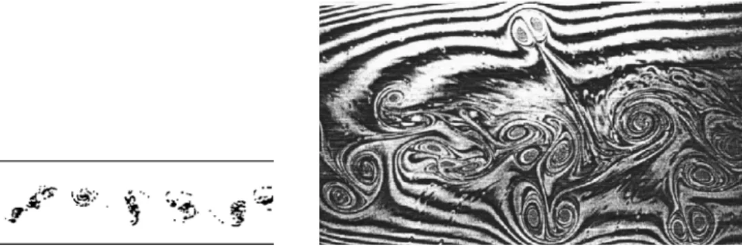
Two-dimensional turbulence has provided a remarkable context for the study of ‘coherent structures’ and the interplay with the classical cascade theories. In the two-dimensional context, the very :rst observations of coherent structures, inferred from direct inspections of numerically computed vorticity :elds, traces backto the seventies. In two-dimensional jets, Aref and Siggia [2] noticed that remarkable vortical structures survived for long periods of time, in conditions where turbulence can be considered as fully developed (see Fig. 1). These numerical observa-tions, appearing after the Brown and Roshko [17] experiment, shed new light on the intimate structure of turbulence, and one may say that today, research in turbulence is still challenged by these early observations. Later, in a turbulent wake produced in a soap :lm. Couder [23] observed structures — vortices and dipoles — keeping their coherence for long periods of time,
and apparently forming the basic elements of the wake (see Fig. 2). These observations were
largely con:rmed by the subsequent numerical and physical studies carried out on the subject [25,85]. McWilliams gave evidence of the formation of vortices, whose lifetimes are hundred times their internal enstrophy, a period exceeding by far any expectation based on traditional ideas of turbulence. Legras et al. [72] showed several long-lived structures, including a superb long-lived tripole in a forced two dimensional turbulent system (see Figs. 3 and 4).
Coherent structures can often be visualized directly on the vorticity :eld, as long-lived ob-jects of generally circular topology, with a simple structure, ‘clearly’ distinguishable from the background within which they evolve. Coherent structure is nonetheless a loose concept and attempts have been made to provide sharp de:nitions, useful for their systematic identi:cation prior to the characterization of their properties. There are several issues raised in proposing a
Fig. 1. Simulation of a two-dimensional jet showing the formation of long-lived coherent structures. Fig. 2. Two-dimensional Von Karman street, formed behind a cylinder dragged in a soap :lm.
Fig. 3. Typical vorticity :eld of a free-decay experiment, obtained several vortex turn-around times after the decay process starts.
Fig. 4. Tripole obtained in a simulation of freely decaying turbulence.
de:nition of coherent structures. For single vortices, it may be diEcult to assume the internal pro:le be smooth since in some situations — during vortex merging for instance — vortices develop a complex intricate structure and their pro:le can be extremely corrugated, especially at high Reynolds numbers. Proposing a vorticity threshold criterium for identifying structures may also raise diEculties at high Reynolds numbers, since Helmoltz theorem stipulates the 9uid particles keep their vorticity level wherever they move.
McWilliams analyzed these issues and proposed an empirical procedure of identi:cation of the vortices [86]. The vortex census proposed by him includes several steps:
1. identify extremas (using a threshold criterion),
2. identify interior and boundary regions (de:ning a threshold for the boundary and check it has a circular topology),
3. eliminate redundancy (checking the structures are separate),
4. test vortex shape (there should be no strong departure from axisymmetry).
Another way of identifying structures is based on the use of Weiss’s criterion. This criterion is discussed in detail by Basdevant et al. [6]. Weiss criterion is based on the remarkthat the evolution equation for the vorticity gradient satis:es the following equation:
d∇!
in which A is the velocity gradient tensor. The eigen values associated to A are calculated as the roots of the following equation:
2=1
4(2−!2) = 4Q ; (16)
where is the strain. Then assuming the velocity gradient tensor varies slowly with respect
to the vorticity gradient, Weiss derived the following criterion: in regions where Q is
posi-tive, strain dominates; the vorticity gradient is stretched along one eigenvector, and compressed
along the other. In regions where Q is negative, rotation dominates, and the vorticity gradients
are merely subjected to a local rotation. Thus, selecting strongly negative Q allows capturing
regions occupied by stable strong vortices, and this o=ers a way for identifying coherent struc-tures, which has the advantage of incorporating some dynamics. In Ref. [6], the hypothesis on which Weiss’s criterion relies is assessed; the relevance of the criterion for analyzing the dynamics of the 9ow is shown, although the criterion is strictly valid only near the vortex core and the hyperbolic points. Progress made to propose a more rigorous criterion, useful for handling dispersion phenomena, has recently been o=ered by Hua and Klein [55]. One may also mention a method, linked to the Weiss criterion, but based on the pressure, for identifying coherent structures [70]. The method is based on the remarkthat the Laplacian of the pressure
is proportional to the Weiss discriminant Q. Therefore, by looking at the pressure :eld, one
may identify regions dominated either by strong rotation or by high strains.
To checkinternal coherence, an attractive method is to determine, in the frame of reference of the supposedly coherent structure [97], the scatter plot (also called the coherence plot),
i.e. the relation between the vorticity ! and the stream function . For a stationary solution,
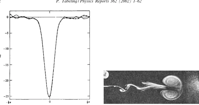
vorticity is a function (not necessarily single valued) of the stream function. Thus, the scatter plot shows a well de:ned line for a stationary structure, and randomly distributed points if the structure undergoes strong temporal changes. The existence of well de:ned lines, which do not evolve for long periods of times, provides a direct visualization of the internal coherence of the so-called ‘coherent structures’. An example of a scatter plot, obtained in a decaying experiment [10], is shown in Fig. 5. Tracking such curves in a turbulent :eld may be a method for identifying coherent structures; however, since one must workin a frame of reference moving and rotating with the structure at hand, this technique is diEcult to implement in practice.
Another technique for identifying coherent structures, based on wavelet decomposition, has been advocated by Farge [35] these last years. It consists of decomposing the :eld into orthonormal wavelet coeEcients, and selecting coeEcients larger than some threshold. Coherent structures correspond to the selected coeEcients, the rest forming the background. Interesting properties have been shown. In the cases considered, the background vorticity is found to be normally distributed, o=ering a favorable situation for theoretical analysis. Also much of the statistics of the :eld is captured by only a few wavelets, which may be interesting for compu-tational purposes.
Determining the stability of isolated vortical structures is a central issue and a diEcult theo-retical problem even for the simplest morphologies. There are some mathematical results, partly reviewed by Dritschel [30]. Circular patches of uniform vorticity are nonlinearly stable; this is important to mention, because the stability of isolated circular vortices opens a pathway for the formation of coherent structures in two-dimensional turbulence. It also marks a di=erence
Fig. 5. Scatter plot (or ‘coherence plot’) obtained in a decaying experiment by Benzi et al. The presence of well de:ned branches reveal the existence of coherent structures, characterized by the same !– relationship.
Fig. 6. Several phases of the axisymmetrization process, transforming an initially elliptical vortex into a circular one.
between two and three dimensions, since the three dimensional equivalent of a two-dimensional vortex — the Burgers vortex — , is observed to be unstable with respect to three dimensional perturbations. In two dimensions, vortices are intrinsically stable, and the emergence of coher-ent structures is easier than in 3D. Elliptical vorticity patches, however, are not stable. The physical mechanism at workis better seen on initially elliptical vortices, as shown in Fig. 6 [57]. Due to the di=erence in rotation rate between the center and the edges, the edges of the vortex is subjected to :lamentation, and after a while, the initially elliptical vortex adopts a circular shape. The overall picture of the monopolar stability has been con:rmed experimentally [40]. More complicated morphologies are mostly out of reach of theoretical analysis, and one must rely on experimental evidence to determine whether a structure is stable or not. In this framework, isolated dipoles and tripoles (such as the one of Fig. 2) are reputed to be stable while pairs of like sign vortices are unstable against perturbations leading to vortex merging.
The internal vorticity pro:les of the coherent structures are mostly controlled by the initial conditions and therefore can hardly be universal (Fig. 7 shows such example of such a pro:le, extracted from [85]). In contrast, the shapes of the coherent structures (more speci:cally the vortices) tend to be circular after a few turnaround times, under the action of the aforementioned axisymmetrization process [87].
The dynamics of a small number of vortices has been studied analytically, numerically and experimentally for several decades. A classi:cation of vortex interactions, involving up to four elements, has been o=ered, in view of providing information helpful for the description of larger vortex systems, prone to sustain fully turbulent regimes [30]. In many cases (i.e. as distances between vortex cores exceeds by far the vortex sizes), the dynamics of vortex patches can be described by using point vortex approximation. The point vortex approximation has been used in a number of cases to study basic phenomena, such as the inverse cascade of energy and the free
Fig. 7. An example of an averaged pro:le of a set of vortices, with negative vorticity, in a freely decaying system. Fig. 8. A dipole formed in a strati:ed 9uid system, loosing 9uorescein behind it as it moves forward.
decay of turbulence [126,10]. The simplest structure involving more than one vortex is the Lamb dipole; the pointwise vortex approximation can be used to estimate their propagation velocity; however, by using this approximation, one does not accurately reproduce the dynamics of the saddle point, located at the rear of the dipolar structure, and across which leaks of vorticity or dye (if the vortices carry dye) can occur [134]. Several aspects of the dipolar structure have been investigated in detail in Refs. [38,39] (Fig. 8).
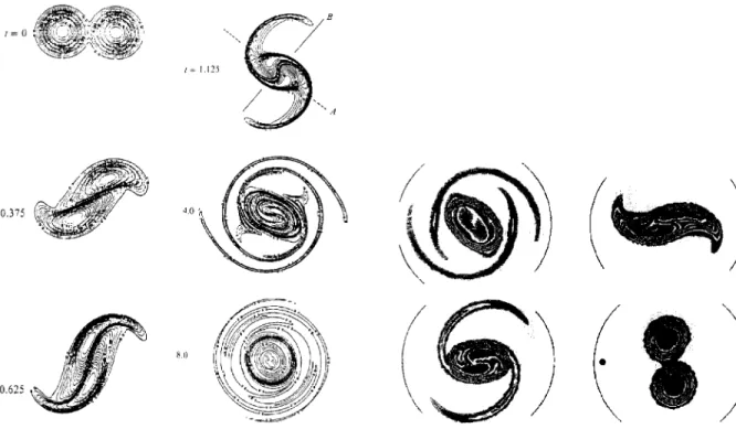
Clearly, some vortex interactions cannot be represented by using pointwise vortices. An ex-ample is the merging of like sign vortices, which plays a fundamental role in the free decay of two-dimensional turbulence, since it drives the formation of increasingly large structures, the most striking characteristics of freely decaying regimes. Vortex merging has been studied along di=erent approaches in the past, and we may say today it is a subtle, rather well documented process. It is subtle because it involves a broad range of scales: as early numerical simulations suggested, vorticity :laments, rapidly lost by the action of viscosity, must be produced for merging to occur. The phenomenon thus involves an interplay between small and large scales. In the particular case of the merging of two identical vortices, it is remarkable that we now have an exact solution of the Navier–Stokes equations [136]; from a mathematical point of view, one thus may consider the problem is solved. However, it is not straightforward to dig out the physical content of the solution, and it is worth considering several concepts devised along the years, for discussing the phenomenon on a physical basis. First, why do vortices merge? Melander et al. [87] propose an instability mechanism, they called “axisymmetrization process” (because the merging will axisymmetrize the system formed by the vortex pair), driven by vorticity :lament formation. They showed that whenever two like-sign vortices are separated
Fig. 9. The six steps of the merging process shown in the paper of Melander et al. (1988). Fig. 10. Experiment, carried out in a plasma, showing the detail of the merging process.
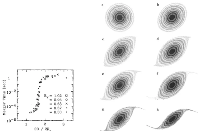
by less than a critical distance, they merge. Far from each other, they do not interact; as they get close, they strain each other, developing thin :lamentation along their edges, and as a result — for energetic or mechanical reasons — the cores get closer and closer, eventually form-ing a sform-ingle structure (see Figs. 9 and 10). Mergform-ing is completed by the smoothform-ing action of viscosity. The notion of critical distance is not straightforward to understand, but it represents well the observations (see Fig. 11). For equal vortices, of circular shapes and uniform vorticity, the critical distance is estimated to be 1.6 time the radius of each vortex. In practice however, merging of unequal vortices is more frequent than the one of equal vortices. One may also mention an appealing description, based on statistical premises, viewing vortex merging as the expression of a maximum entropy principle. I will come backto this theory later.
On the experimental side, we now have detailed analysis of the merging process: by using magnetically con:ned columns of electrons, Driscoll et al. [36] con:rmed many of the features discussed above, in particular the existence of a critical distance; this notion appears through a plot showing that the merging time tends to diverge as the intervortical distance approaches a critical value, consistent with earlier estimates.
Another process involved in the decay phase is vortex break-up, which causes the elimination of the weakest vortices, under the action of the strain exerted by the others. This process is also rather well documented. Idealized cases, with isolated patches of uniform vorticity have been worked out by Moore and Sa=man [93] and Kida [63]. Legras and Dritschel [73] showed
Fig. 11. Experiment showing the divergence of merging time as the intervortical distance increases (by Driscoll et al., 1991).
Fig. 12. Numerical experiment showing that a vortex, subjected to a strain, undergoes distortion, and, above some threshold, break-up.
that vortex breaking is controlled by a critical ratio of the strain rate over the core vorticity of the vortex, and this ratio was found weakly dependent on the vorticity pro:le and, provided the Reynolds number is large, independent of the viscosity (Mariotti et al. [80]) (see Fig. 12). The main lines of the analysis have been con:rmed in physical experiments [109,108,132] (see Fig. 13). Recent progress on the subject has been achieved by Legras et al. [74]. One may also mention an analytical study of the e=ect of the background strain on a population of vortices, well con:rmed numerically by Jimenez et al. [58].
Other processes are involved in turbulent systems, as pointed out by McWilliams [86]: lateral viscous spreading of the vorticity, translation through mutual advection, and higher order inter-actions between vortices; all contribute to reinforce the diversity of two-dimensional dynamics, and the reader may refer to the references listed in the present review, which include descrip-tions of these phenomena (Figs. 14 and 15 depict two steps of the decay of a population of 1000 vortices showing the formation of increasingly large structures, according to McWilliams [86]).
Fig. 13. Experiment, carried out in a strati:ed 9uid, showing the break-up process.
4. Statistics of the coherent structures in decaying two-dimensional turbulence
So much emphasis has been put on the free decay of two-dimensional turbulence that it
sometimes stands as thetwo-dimensional turbulence problem. This is unjusti:ed in my opinion;
we will see in this review that freely decaying systems de:ne a speci:c physical situation, which shares common features but also displays strong di=erences with the forced case. The main di=erence comes from the fact that coherent structures spontaneously pop up in freely decaying systems, whereas they can be inhibited or destroyed in forced systems. In three dimensions, as far as statistics are concerned, there is essentially no distinction between forced and free situations; in two dimensions, this is not so, and in general, a distinction must be made.
Brie9y stated, the problem of the free decay of two-dimensional turbulence is to determine how abundant populations of vortices freely evolves with time at large Reynolds numbers. The vortices may initially be spread at random in the plane, or form a perfect crystal, have Gaussian pro:les or be of uniform vorticity. In all the documented cases, the system evolves towards a state where coherent structures dominate the large scales of the 9ow, and apparently universal features show up. The crude aspects of the process were known in the sixties, but the :rst detailed analysis was performed in 1990, by McWilliams [86]: McWilliams succeeded to disentangle the few elementary mechanisms at work: he showed that in the decay phase, the weakest vortices are destroyed by the break-up process, while the strongest ones merge with other partners, of weaker or comparable strength; these mechanisms generate a re:nement of the vorticity distribution (see Fig. 16). The vorticity distribution thus sharpens as the system decays, but in this process, the most probable vorticity level was observed to remain constant. Driven by a sequence of merging events, the system gradually and unavoidably evolves towards a state where vortices become fewer and larger. Throughout the decay regime, thin vorticity :laments
Fig. 16. Vorticity distributions plotted at various times, fromt= 0 and 40; the distributions change, but the location of the maximum does not appreciably shift during the decay process (same paper as above).
keep being produced, either during merging events, or in the break-up process, developing a vorticity background. At moderate Reynolds number (such as the one of Ref. [86]), they rapidly disappear from the landscape, but at larger Reynolds number, they may nucleate additional small vortices, driven by Kelvin–Helmholtz type instability. Eventually, in current numerical and physical experiments, one typically reaches a state where a pair of large counter-rotating vortices are left in the system, forming the so-called “:nal dipole”. The reader may refer to Ref. [86] for more quantitative aspects.
The problem of the free decay of turbulence is rich, and several issues are embedded in it. What is the structure of the small scales, i.e. those smaller than the initial injection length? Are general cascade concepts relevant to discuss them? What is the ultimate state of the 9ow, appearing at the end of the decay process? Here, I restrict myself to presenting the dynamical evolution of the large scales of the system, i.e. those dominated by coherent structures, a problem on which much has been learnt these last years. The other issues will be discussed later.
The early theoretical analysis of the decay problem, proposing a statistical description, can be found in a remarkable paper by Batchelor [9]; the paper contains the important result that the decay process must be selfsimilar in time, a result which in9uenced all the theoretical approaches developed on the problem. The theory, which does not particularly specify the range of scale it addresses, is expressed in the spectral space. Batchelor’s approach has been reinterpreted in the real space, and for the large scale range, by Carnevale et al. [21]; this interpretation is interesting to consider for o=ering a consistent presentation of the free-decay process. If one constructs an expression for the number of vortices per unit of area, one must write the following expression:
N=f(E; t);
where t is time and E is the energy per unit mass and area, the only invariant surviving, at
large Reynolds numbers, in neutral (i.e. with zero mean vorticity) populations [98]. Dimensional
analysis further leads to the result that the density of vortices decreases as
∼E−1t−2
[9]. The same argument applied to the vortex size, a, and the intervortex spacing, r shows they
must be proportional to time, implying the system expands. This approach has been considered as a cornerstone for a long time. However, with the advent of powerful computers, unacceptable deviations appeared and we had to move towards other paradigms.
The :rst deviations were revealed by McWilliams [86] analysis, mentioned in the beginning of the section. The paper is a numerical study of a population of one thousand Gaussian vortices, located at random in a square with periodic boundary conditions. The number of vortices, the size and the intervortical distances were measured and the results are shown on Figs. 17 and 18. One could see well de:ned power laws, but the exponents were found clearly incompatible with Batchelor’s theory.
The exponent for the vortex density for instance, was found equal to −0:7, a value
incom-patible with Batchelor’s expectation (leading to −2); a similar comment can be made for the
size (growing as t0:2 instead of t) and the mean separation (increasing as t0:4 instead of t).
To account for this observation, Carnevale et al. [21] o=ered the idea that another invariant must be dug out, and this gave rise to the ‘universal decay theory’ [101]. More speci:cally,
Fig. 17. Decay law for the number of vortices, found by McWilliams [86]; the results show evidence for the existence of a power law, with an exponent close to −0:70.
Fig. 18. Power laws obtained for the vortex density , size a, intervortical distancer and extremal vorticity.
they proposed to take the extremum vorticity of the system !ext as the missing ghost invariant.
There is no rigorous justi:cation for this assumption, but a physical plausibility, supported by numerical observation. Indeed in the inviscid limit, the maximum vorticity level, as any other levels, is conserved. But in the problem we address here, it is not clear the Euler equations
provide an acceptable approximation. The constancy of !ext is physically justi:ed by the fact
that the strong vortices undergo two types of situations; either they wander in the plane or they merge; in none of these situations, their internal circulation has an opportunity to substantially decrease. Therefore, it is plausible, on a physical basis, to consider the extremum vorticity as a constant. This argument is supported by the observation that the most probable vorticity level remains (approximately) constant during the decay phase [86].
The next step is to estimate various quantities of the problem. The following equations are written
Z∼!2
exta2 ; (17)
E∼!2
exta4 (18)
in which Z is the enstrophy per unit area and E is the energy per unit mass and area. The
estimate for the energy neglects logarithmic contributions; this delicate omission is discussed in some detail in Ref. [139]. Thus, using the above relations, along with the constant extremum vorticity assumption, and further hypothesing power laws, Carnevale et al. [21] obtained the
following laws for the density of vortices , the vortex radius a, the mean separation between
distribution: ∼l−2t
T
−!
; a∼l
t T
!=4
; r∼l(t=T)!=2; u∼√E ;
Z ∼T−2t
T
−!=2
; Ku∼
t T
!=2
(19)
in which length l and time scale T are de:ned by
l=!−1 ext
√
E; T=!−1
ext : (20)
The exponent ! is not determined by this theory, but, once it is :xed, all the power law
exponents of the problem are set. Numerical studies, either of the full Navier–Stokes equations
or of point-vortex models, have consistently obtained power laws, with values of ! ranging
between 0.71 and 0.75 [21,139,86].
Concerning the physical experiments, early investigations [24,53,46] revealed the essential qualitative features of the decay process, but could not provide precise determinations of what-ever exponent involved in the problem. Owing to the progress made in digital image process-ing, the situation changed in the last decade and now, accurate measurements are currently performed on two-dimensional decaying systems [102]. One may refer to a study of decay regimes performed in electromagnetically driven 9ows, which yielded reliable data, in good quantitative agreement with the numerical simulation [47]. Examples of such data are shown in Figs. 19–21. In this case, the decay process stretches over a period of time hardly exceeding 25 s, representing 10 initial turnaround times. Despite this limitation, scaling regimes take place rather neatly, and the related exponents could be quite accurately determined. Agreement with the aforementioned numerical studies was obtained, and this reinforced the consistency and robustness of the “universal decay theory” framework.
! thus appeared as a crucial exponent and several theoretical assaults have been given to
determine its value [116,49,133,1]. Pomeau proposed a derivation that yields != 1, arguing for
lowering corrections [116]. On the other hand, using a probabilistic method to describe the motion of vortices in an external strain-rotation :eld, it has been suggested that the value of
! depends on initial conditions [49]. In a related context, the 2D ballistic agglomeration of
hard spheres with a size–mass relation mimicking the energy conservation rule for vortices, the
value != 0:8 is derived under mean-:eld assumptions [133]. Further, in another possibly related
context, that of Ginzburg–Landau vortex turbulence, the value !=3
4 has been proposed [1].
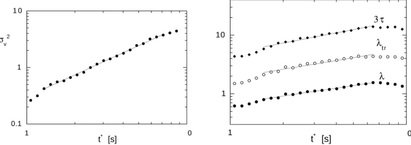
Recently, progress was made on the characterization of the decay process [47]. The mean
square displacements 2
v of the vortices, the mean free path , the collision time $, have
been measured in a physical experiment, and the following power laws have been found (see Figs. 22 and 23):
2
v ∼t with v∼1:3±0:1;
∼t0:45±0:1; $∼t0:57±0:1: (21)
The vortices thus do not undergo Brownian motion in the plane, but possess a hyperdi=usive motion, with an exponent equal to 1.3. On physical grounds, it is clear that this dispersion law,
Fig. 19. Three steps of the decay process observed in a physical experiment, in a thin layer of electrolyte, where the vortices are driven by electromagnetical forces.
and the related exponent (we call ) are linked to the decay problem. The authors of Ref. [47]
argue that a relation between the mean square displacement exponent and the decay exponent,
!, holds; it is expressed by the following formula:
= 1 +3
4! : (22)
This law is obtained by using standard relations of kinetic gas theory (assumed to be appli-cable for the problem at hand). In Ref. [47], the above relation appears well supported by the
1 0 100
N(t*)
t* [s]
1 10
1 1 0
2 3 4 5 6 7 8 9 1 0
t* [s]
N
r
a
Fig. 20. Number of vortices with time obtained in the physical experiment.
Fig. 21. Additional data, showing the vortex size, and the intervortical distance with time, in the physical experiment.
0.1 1 1 0
1 0
σv2
t* [s]
1 10
1 0
t* [s]
3 τ λt r
λ
Fig. 22. Temporal evolution of the squared averaged distance between vortices, obtained in a physical experiment. Fig. 23. Temporal evolution of various quantities, characterizing the evolution of a system of vortices: collision time, mean free paths.
experiment. According to this, both the dispersion and the decay problem seem to be the two faces of the same coin and one may askwhich of them is the more amenable to theoretical understanding.
The presentation emphasizes on exponents, since their existence was implicitly admitted in most of the recent workmade on the problem. However, one may consider that the situation is not fully settled; recent workrevealed log periodic oscillations on the temporal decay of the number of vortices [48]; the authors further argue complex exponents must be used to represent the underlying processes. On the other hand, numerical results obtained by Dritschel [31], using
vortex surgery technique, challenged the existence of power law behavior. There are several consequences of this result, one of them being that power laws may breakdown at extremely large Reynolds number. On the experimental side, the “universal decay theory” is generally considered as :tting well the experimental observations; however, one must mention a recent work[135] which suggests that in the experiment, the walls may have a sizeable e=ect in the determination of the exponents.
Concerning the decay problem, we are thus left at the present time with an elegant phe-nomenological theory (“universal decay theory”) which turns out to represent consistent sets of numerical and experimental observations. In this framework, despite several attempts, the fundamental exponent governing the process is still unexplained. On the other hand, moving further away from phenomenology would probably be desirable, but at the moment, solving the decay problem from :rst principles appears as a formidable challenge theorists do not seem to rush out to tackle.
5. Equilibrium states of two-dimensional turbulence
As we discussed above, freely decaying two-dimensional turbulence evolves towards a state where eventually large structures arise, coexisting with a featureless turbulent background, formed by a collection of short lived vortex :laments. This has been shown for the turbulence decay problem, involving initially abundant vortex populations, and this is also true for systems initially composed of a few structures. Examples are displayed on Figs. 24–26, or can be found in [144,2,24,84–86,11,134,53,137]. One sees systems undergoing complicated evolutions, until eventually a steady state takes place, characterized by the presence of a few structures. The :nal patterns are not universal — their shapes sensitively depend on the boundaries and the initial conditions. The question is whether theory can account for them.
From the observations, it is appealing to consider that the :nal state is a “vorticity melasse”, resulting from the mixing of the many elementary vorticity patches de:ning the initial state; along this line of thought, one is tempted to develop an analogy with thermodynamics, so as to interpret the :nal state as an equilibrium state, which would maximize some entropy. This intuitive idea is, however, not straightforward to substantiate. It has been :rst formal-ized by Onsager, for point vortices systems, i.e. in a context where the analogy could be worked out rigorously [107]. The Hamiltonian structure of the problem and the presence of a Liouville theorem (given by Helmhotz theorem) allowed to calculate equilibrium states, in the same way as in statistical physics. For the problem at hand, the canonical variables are the cartesian coordinates of the positions of the point vortices. Onsager found various possibilities, depending on the initial conditions. Among them, negative temperature states, which arise as a consequence of the :niteness of the phase space; those states are in form of clusters of like signed vortices, coexisting with regions where weakvortices are ‘free to roam practically at random’. In this problem, entropy is gained by randomizing weakvorticity regions, and clusters are formed so as to conserve the total energy. This theory brought an illuminating way to ac-count for the spontaneous formation of coherent structures in 2D 9ows, as repeatedly revealed experimentally and numerically. Onsager’s theory conveyed new concepts in hydrodynamics and inspired, for four decades, a considerable number of contributions [69]. The theory was further
Fig. 24. Evolution of a system of vortices obtained by Matthaeus et al. (1991), showing the formation of the “:nal dipole”.
Fig. 25. Evolution of a vorticity strip towards the formation of a chain of vortices (after Sommeria et al., 1991).
extended to magnetohydrodynamic 9ows and plasmas, and attempts were made to use it for the three-dimensional problem. This interest is probably motivated by the possible relevance of this approach to hydrodynamic turbulence but also — as quoted in Kraichnan and Montgomery’s review [69] — by the fact that we deal with a “bizarre and instructive statistical mechanics”, which makes it interesting in its own right.
There is a number of theoretical issues involved in Onsager’s theory, related to the ergodicity assumption, the existence of a critical point, the pair collapses, the high and low wave-number limits, and they are reviewed in detail in Ref. [69]; also we may mention an excellent, more recent, pedagogical review by Miller et al. [89]; we comment here on the point vortices ap-proximation, which a=ects the practical interest of the theory — I mean its relevance to explain observations. As noted by Pomeau [115] point vortex systems may provide a theoretical frame-workfor super9uid turbulence, where vorticity is quantized into :laments, 1 A in diameter, with a prescribed circulation, but for ordinary 9uids, the discrete approximation is constraining in the sense that it precludes the possibility to compare the theory with the experiment. The problem
Fig. 26. Evolution of a vorticity pattern towards the formation of a dipole, in a periodic box (after Segre et al.).
of working with discrete vortices is that one has an in:nite number of possibilities to construct a given initial continuous vorticity :eld [92]; as a consequence, by using Onsager’s theory, one gets an in:nity of possible equilibrium states; there is thus no way to make a quantitative contact between this approach and ordinary 9uids, and a qualitative comparison is in practice extremely limited.
The desire to cross the bridge between discrete and continuous vorticity :elds has stimulated a number of works, well reviewed by Kraichnan and Montgomery Refs. [69] and Miller et al. [89] and more recently by Brands [16] and Segre et al. [127]. Assuming negative temperature, and a two-level initial vorticity :eld, Montgomery and Joyce [91] proposed to de:ne the vorticity as a local average of the pointwise vorticity :eld, under the assumptions that the vortex number density slowly varies with the position. The set of equilibrium states found under this assumption is governed by the equation
∇2 +%2sinh(&‘a ) = 0; (23)
where is the equilibrium stream function, % is a constant and & is a free parameter,
corre-sponding to a temperature. Interestingly, this theory leads to a universal relation between the locally averaged vorticity and the stream-function, in form of a sinh function. This sinh function turns out to :t well the actual ultimate states observed in a number of experiments.
Another approach has been to workin discrete truncated Fourier spaces. The truncated system is Hamiltonian and has a Liouville theorem, so that one may calculate statistical equilibrium states, using Fourier coeEcients as the conjugate variables. In this approach, the equilibrium state is found as the gravest mode (i.e. with the lowest wave-number) compatible with the boundary conditions. Formally, at equilibrium, the vorticity is found proportional to the stream-function. This proposal has been called the ‘minimum enstrophy principle’ since, in this problem, the equilibrium state turns out to minimize the enstrophy at constant energy [76]. A related concept is the ‘selective decay’, stipulating that freely evolving two-dimensional systems decrease their
enstrophy at a rate much higher than the energy. The theory is appealing in its simplicity, and qualitatively reproduces well the trends observed in decaying systems. However, the linear relationship between vorticity and stream-function is generally not observed. In many cases, sinh functions or hyperbolic functions characterize the scatter plot of the :nal states. The theory can also lead to unphysical predictions. The minimum enstrophy approach is discussed in several places and the reader can refer to Kraichnan–Montgomery’s review [69] to have a detailed account of this work.
Ten years ago, a statistical theory, tackling the discretization problem in a di=erent way, has been worked out [88,120]. The key step has been to introduce a mesoscopic scale over which the stream function could be treated as uniform, and a local determination of the statistical ensembles could be achieved. In this context, the authors [88,120] calculated analytically the maximum entropy states, under the constraints of conserving the energy and the vorticity distribution, i.e. only the invariants which survive after coarse graining. The statistical theory provides, as
a result, a relation between the averaged vorticity :eld !(x) and the stream function (x)
which fully de:ne the equilibrium state. At variance with the previous theories, there is no free parameter in the solution; except in special cases, the form of the relation vorticity — stream function (the so-called scatter plot), requires an iterative procedure to be determined. Here, we present the essential steps of the calculation leading to the result. The :nal equilibrium for a
distribution of discrete vorticity levels ai of vorticity, is found by maximizing a mixing entropy
de:ned by S=−
i
pi(x) ln(pi(x)) dx ;
where pi(x) is the probability of :nding the level ai at the location x. By introducing the
Lagrange parameters & and )i, respectively, related to the conservation of the energy E and
initial distribution of vorticity Ai, and prescribing that the :rst order variation of S vanishes,
one :nds that the equilibrium vorticity :eld !(x) and stream function (x) are given by
!(x) =
i
aipi(x) =
i
aiexp(−&aZ(i (x)) −)i) ; (24)
Z( ) being the normalization factor of the probability distribution. To compute the equilibrium
spatial vorticity distribution, one needs to solve the following set of equations: E= 12
! dx ; (25)
Ai=
pi(x) dx ; (26)
!=−O ; (27)
associated with the boundary condition = 0. In the above equations, the set of Ai, prescribed
by the initial conditions, is known.
It is possible to :nd the structure of the solutions to this system, in con:gurations of great simplicity. For instance, the case of two-dimensional 9ows in a closed rectangular domain (with
Fig. 27. Final states obtained in a plasma experimented by Fine et al. They are in the form of regular lattices of vortices. The dissipation is low enough to investigate thousands of turnaround times, i.e. more than the most conservative numerical simulations.
periodic or rigid boundary conditions), with initial uniform vorticity can be solved. The solution is [131]
!=−O =1 +)sinh()cosh(*+*+**) )
in which all the parameters, i.e. *; *; ) can be calculated using the initial conditions (actually
the taskis not simple). There is no free parameter. It is also worth noting that the sinh Poisson is recovered in the limit of dilute vorticity. It has thus been suggested the sinh Poisson is a particular case of a more general framework.
Nonetheless, the resolution of the system in more realistic cases, along with the determination of the constants in situations such as the previous one, are not straightforward and for years, the numerical pathway for obtaining equilibrium states was ineEcient; this diEculty was solved by the advent of ingenious numerical procedures [140]; the procedure devised by Whitaker and Turkington [140] is iterative and involves the following steps:
1. Compute a set of Lagrange parameters from the vorticity :eld and the related stream function form (25) and (26).
2. Determine the corresponding probability distribution according to Eq. (24). 3. Solve (27) for the new calculated vorticity :eld.
4. Return to :rst step.
The procedure is iterated until the convergence of all parameters is completed. The reader may refer to [59] for examples of applications (other examples can be found in [26,89]). In practice,
the result is insensitive to the precise choice of n.
This theory could be confronted by experiments; it turned out to provide, in several case, predictions agreeing, even at some quantitative level, with the observation: for example, the cases of the jet and the mixing layer, yields good consistency between the theory and the simulation [130,131]. The theory predicts the existence of phase transitions, involving symmetry breakings, as the energy or geometrical factors are varied. Some of them have been found experimentally, consistently with the theory, in a two-dimensional circular mixing layer, [27]. The theory predicts the merging of two-like sign vortices, which is observed, provided they are closer than some critical distance (we will come backto this point later); some deviations have been pointed out in a series of experiments using plasmas [56], while acceptable agreement was shown in another case [82]. It would, however, be incorrect to consider that agreement is the rule. In several cases, it appeared that the theory misses some important features found experimentally. In [37], some observed states — such as vortex crystals of Fig. 27 — appear incompatible with the theory, as worked out in the original papers. An experimental study, done on the decay of
Fig. 28. Final states obtained in a physical experiment, and detailed comparison with the theoretical predictions of Robert-Sommeria.
systems of vortices, and comparing the prediction with the observation on a quantitative basis, obtained discrepancies between theory and experiment — in some cases at qualitative level [82,60] (see Fig. 28). A striking confrontation has been carried out by Segre and Kida [127]. Oscillatory states have been found as :nal states in a number of situations (examples are shown in Fig. 29). This is incompatible with the theory, which expects the :nal state to be stationary in all cases; in the same study, it is shown that the :nal state is not uniquely determined by the vorticity distribution and the energy level: two di=erent two-levels vorticity patterns, with approximately the same energy have been observed to lead to di=erent :nal states; this is also incompatible with the theory.
Whether we like it or not, the existence of situations where the theory fails to predict the ul-timate state obviously generates a number of questions. There are technical issues, but the most critical question is ergodicity. Is is legitimate to assume ergodicity? Does the system investigate all the accessible phase space with equal probability, or can it be trapped for long in a part of it? Is the notion of equilibrium state relevant for interpreting experiments? These points have been discussed in several papers in considerably more detail and in more technical terms than herein (see [69,89,115,16]). The issue can be illustrated by the two like-sign vortices problem; in this case, statistical theory (I could say all statistical theories) predict the vortices to merge, whereas experiments show that above a critical distance, the vortices remain separated for ever (‘ever’ means thousands of turn-around times); in the frameworkwe consider here, we may interpret this observation as an inhibition to reach an equilibrium state. Why can it be so? Pomeau [115] pointed out that the origin of randomness in 2D 9ow is far weaker than in ordinary statistical systems: as the system evolves, at :nite Reynolds number, the dynamical role of the vorticity :laments gets weaker, whereas the large structures tend to form stable circular regions. The small scale 9uctuations thus tend to collapse and consequently, the possibility to reach an equi-librium state, as in ordinary statistical mechanics, becomes questionable. One may askwhether increasing the Reynolds number favors ergodicity. At the moment, there is no evidence it can
Fig. 29. Oscillatory states found as the :nal states in simulations initiated with two-levels vorticity patterns. The right :gures are the vorticity distributions and the scatter plots. The nonstationary nature of the state is made visible by the thickness of the curve in the scatter plot.
be so. It appears that in two-dimensional systems, there is no mechanism ensuring ergodicity in general, and assuming ergodicity seems to be in too many cases a misleading premise. A discus-sion on ergodicity from a more dynamical prospect has been given by Weiss and McWilliams [138]; these authors underline the existence of dynamical pathways, which control the decay phase. After the decay phase is achieved, the 9uctuations have declined, and the system ceases to evolve. According to this view, the :nal dipole is seen as the completion of a selfsimilar process, rather than an equilibrium state resulting from the mixing of the vorticity patches. The relevance of this approach has been underlined in a physical experiment [82]. Note :nally that one can :nd cases where ergodicity does not hold [138].
Several criteria have been o=ered to determine the validity of the ergodicity premise [92,16]. One may perhaps propose another one, based on physical considerations, and expressed in terms
of a dimensionless parameter P de:ned by P=E=L2Z
0 ;
where L is the box size con:ning the 9ow and Z0 is the initial enstrophy; this parameter is
the natural dimensionless quantity one may introduce to discuss the problem (see for instance
[115,89,19]). As P is small the system must gain much entropy to reach an equilibrium state,
and this involves substantial mixing, diEcult to achieve in two dimensions. On the other hand,
when P is high, the system does not need to gain much entropy to reach equilibrium, because
the energy level is high, and the number of accessible states is low; thus in this case, moderate mixing may be suEcient for the system to approach an equilibrium state and we may expect that statistical theory provides useful predictions. These rough ideas have been illustrated for
vortex arrays [83]. Just to :x the ideas, one :nds that deviations appear as P gets smaller than
5×10⁻³; this may de:ne a cross-over between two situations, one favorable for equilibrium
states to be reached, the other unfavorable. A possible paradox of this situation is that statistical theory works better when the entropy tends to become irrelevant.
Recently, several modi:cations have been brought to improve and extend the original theo-retical framework. The idea is to de:ne bubbles within which ergodicity holds and outside of which the 9ow is deterministic [20]. A similar idea was proposed earlier by Driscoll, in view of proposing a more realistic version of minimum enstrophy theory [56]. This adjustment allows to improve the consistency between theory and experiment, at the expense of introducing a substantial complication.
To conclude, one may say that at the moment, the statistical approaches have not been proven yet to o=er a more than qualitative frameworkfor the interpretation of experimental observations. It seems that we are in a situation where unresolved issues are hanging, and the theory has to face formidable diEculties to make further progress. Do these theories correctly indicate the direction of the arrow of time? This is not ascertained in general. Nonetheless, the conceptual frameworkis appealing and certainly deserves stronger interest than now in the 9uid dynamics community.
6. Inverse energy cascade
The concept of the inverse energy cascade traces backto Kraichnan [67] who :rst proposed that energy and enstrophy can cascade in two dimensions, a possibility often ruled out before him. In two dimensions, one has the conservation of the vorticity of each 9uid parcel in the inviscid limit. These conservation laws imply the existence of two quadratic invariants: the energy and the enstrophy. These two constraints led Kraichnan to propose the existence of two di=erent inertial ranges for two-dimensional turbulence [67]: one with constant energy 9ux extending from the injection scale toward larger scales and one with constant enstrophy 9ux extending from the injection scale down to the viscous scale. The :rst one is known as the inverse energy cascade, and the other as the enstrophy cascade.
The argument leading to this double cascade picture is better given in the Fourier space because the relation between energy and enstrophy is straightforward; it unfortunately does not :nd a simple expression in the real space, making it hard to explain physically in accurate terms.