Spatial data analysis: retrieval,
(re)classification and measurement
operations
In chapter 5 you used a number of table window operations, such as calculations, aggregations, and table joining, in the analysis of attribute data. In the previous chapter you have seen the most important image processing tools that ILWIS provides for the analysis of satellite data. In this chapter, and also in chapters 8 and 9, attention will be paid to other data analysis tools, specifically for maps.
ILWIS provides a wide range of tools to perform operations on spatial data. These tools enable you to transform your input data into useful information.
There are several ways in which the data analysis tools can be subdivided. We have chosen the subdivision as suggested by Aronoff, 1989 (see Preface).
Retrieval, (re)classification & measurement operations
These operations mostly form the starting point in the data analysis process. They enable you to explore your data, without making changes to the location of spatial elements and without creating new spatial elements.
- Data retrieval involves the selective search of data.
- Reclassification involves the (re)assignment of thematic values to categories of an existing map.
- Measurement operations involve the measurement of distances between points, lengths of lines, area and perimeter of polygons, determination of volumes and counting.
All operations in this category are performed on a single vector or raster map, often in combination with attribute data.
Retrieval, (re)classification and measurement operations will be treated in this chapter. Overlay operations
This group of operations forms the core of many GIS projects. With the help of these operations, a number of maps are combined and new information is derived. New spatial elements are created. This set of operations is only performed on raster maps in ILWIS.
ILWIS has a powerful tool to combine maps, called Map Calculation. Many maps can be combined at the same time using arithmetic, relational, or conditional operators and many different functions in formulas that you can type on the
Command line of the Main window.
Two other important tools to overlay raster maps are the Cross operation, which calculates the frequency of occurrence of all possible combinations of two maps, and the use of a two-dimensional table, which is a matrix in which the user can define how all classes of two maps should be combined.
Overlay operations will be treated in the next chapter, including an extensive demonstration of Map Calculation.
Neighborhood operations
Where the overlay operations only consider the combination of raster cells in different maps at the same location, the neighborhood operations evaluate the characteristics of an area surrounding a specific location. These operations make use of small windows of 3x3 cells, which perform one calculation on a center raster cell and its eight neighbors. The result is stored in the central cell. Four types of
neighborhood operations will be treated in chapter 9: Neighborhood operations in
Map Calculation, Filtering (as was shown in the previous chapter for satellite images, but now applied to thematic maps), AreaNumbering and Distance calculation.
Map Calculationcan be used for many operations. Map Calculationwill be treated as a block of exercises in the next chapter.
Before you can start with the exercises, you should start up ILWIS and change to the subdirectory C:\ILWIS 3.0 Data\Users Guide\Chapter07, where the data files for this chapter are stored.
•
Double-click the ILWISicon on the desktop.•
Use the Navigatorto go to the directory C:\ILWIS 3.0 Data\Users Guide\ Chapter07.7.1 Retrieval using the pixel information window
Data retrieval involves the (selective) search, manipulation and output of spatial data and/or attribute data. Retrieval operations can be subdivided into the following groups:
- What is at...?
To find out what is present at a particular location. Reading of the contents of maps and related attribute tables at specified XY-coordinates. In ILWIS, the pixel
information window can be used to read the values from vector and/or raster maps, with their accompanying tables.
- Where is...?
Retrieval of spatial data (points, lines, polygons or mapping units in a raster map) to find an answer to questions such as: “Where are the forested areas?”
The pixel information window is used to interactively inspect coordinates, class names, IDs or pixel values, in one or more maps and map-related tables. The pixel information window shows information for the mouse pointer’s position in a map window. In chapter 2, the functionality of the pixel information window was already introduced to you.
To view attribute information in a pixel information window, you have to add one or more maps that have an attribute table to the pixel information window. You should display at least one map in a map window.
In this exercise you will start to read the information from four polygon maps
Geology, Geomorphology, Landuse, and Catchment(watersheds in the mountain area) together with their tables. In the map window, you will display a false color composite made of the TM bands 4, 3 and 2.
For this exercise we have also prepared some maps that are made from the segment map Contour: a Digital Elevation Model (Dem) and a slope map (Slope). The
•
Open raster map FCC.•
In the map window open the Filemenu and choose Open Pixel Information.•
Open the Helpmenu in the pixel information window and select the com-mand Help on this window. Click the hypertext word: Introduction.•
Close the Helpwindow when you have finished reading the help on the pixel information window.☞
•
In the Catalog, select the polygon maps Geology, Geomorphology,Landuseand Catchment(hold down the Ctrl-key) and drag them to the pixel information window.
•
When you move the mouse pointer in the map window, you will see informa-tion on these maps in the pixel informainforma-tion window.DEM shows the altitude of each raster cell, and the slope map shows the slope angle in degrees. The procedure to construct such maps will be explained in chapter 10.
Firstly, the pixel information window receives the XY-coordinate from the mouse pointer (located in a map window) or the digitizer cursor (located on a referenced paper map on the digitizer). Then, for this received coordinate, information of all raster, polygon, segment and point maps that were added to the pixel information window is retrieved and displayed simultaneously. For raster maps, the retrieved information refers to the pixel pointed at with the mouse pointer, hence pixel info.
The three polygon maps do not cover the entire area displayed in the false color composite. If you move to the right of the image, you will see that the information from the geologic and geomorphologic maps is missing (it says for the maps: ? outside map, and for attribute data: ?).
You can use pixel information to become familiar with the data and to find out certain relations between one map and another.
To find such relations it may be useful to display these maps on top of the false color composite.
For more information on how to manage data layers we refer to chapter 2 and to the
ILWIS Help topic Basic concepts: Layers in a map window.
•
Also add the raster maps Demand Slopeto the pixel information window. You can do this for instance by using the Add Mapcommand in the Filemenu of the pixel information window.
•
Position the mouse pointer in the map window.☞
•
Click somewhere in the map window. You can see the corresponding informa-tion of that locainforma-tion in the pixel informainforma-tion window.•
Move the mouse pointer through the map to continuously display the infor-mation.☞
•
Select the four polygon maps Geology, Geomorphology, Landuse, andCatchmentin the Catalogand drag them to the map window.
•
When the Display Options - Polygon Mapdialog boxes appear, specify:Boundaries Onlyand choose for:
Catchment(Boundary Color: White)
Geology(Boundary Color: Magenta)
Geomorphology(Boundary Color: Yellow)
Landuse(Boundary Color: Green).
All layers are now displayed in different colors on top of each other. Let us only display one layer: Landuse.
Now you only see the green boundary lines of the land use polygons on top of the false color composite.
By manipulating layers that are displayed in a map window and information shown in the pixel information window, you can easily evaluate your data.
When you finish the exercise:
•
In the Layer Managementpane, clear the Showcheck boxes of the layersGeology, Geomorphologyand Catchment.
☞
•
Close the pixel information window and the map window.☞
•
Position the pixel information window and the map window in such a way on your screen that you can easily see both.•
Move the mouse pointer through the map, while keeping the left mouse but-ton pressed. You can read simultaneously the land use information in the map, and all other information from the pixel information window.•
Find the answer to the following question:What is the predominant geological unit that is used for irrigated agriculture?
☞
•
Find the answer to the following questions (use the information in the pixel information window, and change the displayed polygon layers usingLayer Managementin the map window as you wish):- What is the predominant land use type on the alluvial fans, just north of the city of Cochabamba?
- What is the maximum elevation at which we still find forest?
- For which catchment do we not have geological nor geomorphologic infor-mation?
- Are there parts of the city of Cochabamba that may be flooded?
- Which one of the geomorphologic zones (column zonation) has the steep-est slope? In which range are these slopes?
7.2 Retrieval of information by displaying attributes
The pixel information window allows you to retrieve information for the XY-coordinates where the mouse pointer is located. However, in many cases you do not want to have the information for one location only, but for an entire map.
In this exercise you will learn how to display attribute data from a column in a table, which replaces the original information in a map.
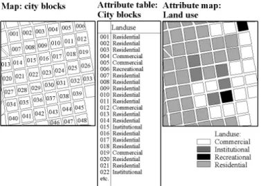
The Cityblockmap is used as an example. In chapter 5 (attribute data handling), you worked with table Cityblockwhich contains information such as area, land use, district number, population and population density for each city block.
The Cityblockmap is now displayed in seven different colors. Each city block has a unique code.
The polygon map window with the Edit Attributespane docked into the map window is shown in Figure 7.1.
As you can see, there is information on each city block. The white areas (the roads in-between the city blocks) have no information. Although you could, for example, double-click each city block to find out its land use, it is obvious that this is a tedious procedure. ILWIS has a more flexible way: you can display a map by one of its attributes.
•
Open table Cityblockand inspect the properties of the various columns, by double clicking the column titles. As you can see, the column Landusehas a class domain (City_Landuse), the column Districthas an ID domain (District), and the columns Area, Population, andPopulation_Densityall have a value domain. When you have seen the properties of the columns, close the table again.
•
In the Catalog, double-click polygon map Cityblock. Accept the defaults in the Display Options - Polygon Mapdialog box and click OK.☞
•
Click some of the units in the map and find out their codes.•
Double-click a unit in the map to find information in the attribute table that is connected to the map.If you wish you can drag the Edit Attributeswindow into the map window, and dock it.
☞
•
Close the Edit Attributepane by clicking the cross in the upper-right.Column Landusehas a class domain (called City_Landuse) which has a representation (City_Landuse).
The map Cityblockis re-displayed, but now in such a way that the colors no longer represent the various codes of the city blocks. The colors now show the land use types according to representation City_Landuse.
Figure 7.1: A polygon map window with both the Layer Management pane and the Edit Attribute pane docked in the map window.
•
In the Layer Managementpane of the map window, double-click the mapCityblock. The Display Options - Polygon Mapdialog box is opened.
•
In the Display Options - Polygon Mapdialog box select the check boxAttribute. Now a list box appears to the right of the word Attribute, contain-ing columns of the attribute table Cityblock.
•
Select the column Landuse. This column contains the dominant land use type of each cityblock.•
Select the option Representation. The representation City_Landusewill appear in the list box to the right of the word Representation.☞
•
Click OKin the Display Options - Polygon Mapdialog box.Displaying a map by one of its attributes allows you to get a good idea on the distribution of the different attribute values throughout a map.
You will display another attribute of the Cityblockmap: District. Each city block forms part of a cadastral district of the city. The Districtcolumn uses an identifier domain.
Now the map Cityblockwill be shown by the attribute population density. The column Population_Densityuses a value domain
You can display both raster and vector maps by one of its attributes, as long as the map has a class or ID domain and an attribute table is linked to the map. This is defined in thePropertiessheet of the map.
Retrieval with a mask
Finally, you will have a look at some other useful options in the Display Options
dialog box that can help you to evaluate the data.
We will switch to another example: the land use map of the region around the city of Cochabamba, called Landuse. You can selectively display units in a map, e.g. only the land use type Forest.
•
Click on the different units in the map. You can see that for each city block the land use type is shown as well as the code of the city block.☞
•
Click with the right mouse button while the mouse pointer is in the map win-dow. Select Display Optionsfrom the context-sensitive menu and click on the polygon map name Cityblock.•
Select the check box Attribute, and select column District. Since this col-umn uses an identifier domain, you cannot select a representation. Instead, you can display districts in 1, 7, 15 or 31 colors.•
Select the option Multiple colors, and 15. Click OK. Now the map is dis-played according to the districts of the city.•
Check the content of the map by clicking a few different units.☞
•
Change the options in the Display Optionsdialog box in such a way that the attribute Population_Densityis displayed with the RepresentationPseudo. Stretch between 0and 1000.
•
Check the contents of the map window.•
Close the map window after you have finished the exercise.Only the land use unit Forest is shown in the map window. Suppose you want to show the following four units: Bare rock, Bare soils, Agriculture, and
Agriculture (irrigated). Instead of typing full names or codes you can use wildcards: the asterisk *to replace zero or more characters, and the question mark (?) to replace one character.
A mask can be used to selectively display vector data. For maps with many different units this can be quite useful, e.g., to show specific contour lines.
For more information about using wildcards in Mask, we refer to the ILWIS Help
topic How to use masks.
•
In the Catalog, double-click polygon map Landuse. The Display Options -Polygon Mapdialog box is opened.•
Select the check box Mask, type the class name Forestin the appearing text box and click OK.☞
•
Open the Display Optionsdialog box of polygon map Landuseagain.•
Select the check box Mask, and type the following search strings in the appearing text box: Bare*,Agri*•
Click OKin theDisplay Options – Polygon Mapdialog box.•
Now only four units of the map are displayed: Bare rock, Bare soils,Agricultureand Agriculture(irrigated).
•
Close the map window.☞
•
In the Catalog, double-click segment map Contour.•
In the Display Options – Segment Mapdialog box, select the check boxMask, and type the following search strings in the appearing text box: 30*,
31*, 32*, 33*, 34*.
•
Select the check box Infoand click OK. Only the contour lines from 3000 to 3440 are displayed.•
Double-click the map Contourin the Layer Managementpane.•
In the Display Options – Segment Mapdialog box, select the check boxMask, and type the following search string in the appearing text box: ??00.
•
Click OKin the Display Options – Segment Mapdialog box. Only the hundred meter contour lines are displayed.•
Close the map window.Summary: retrieval operations
- In the previous exercises methods were shown that could be used to retrieve information from maps and from the connected attribute tables.
- In section 7.1, you practiced with the pixel information window. The pixel information window allows you to read data from many maps and tables simultaneously, for the XY-coordinate that you point at with your mouse pointer. - In section 7.2, you displayed a map by one of its attributes. An attribute table
should be linked to the map, and the column values that you show may use a representation.
- Both vector and raster maps that have a class domain, an identifier domain (ID domain) or the Unique ID domain, and that have an attribute table linked to it, have the possibility to display attributes instead of their own classes or IDs.
- Displaying a map by one of its attributes is useful to investigate the spatial distribution of attribute information, without the need of generating a new map. - You can also use a Maskto selectively display some classes, IDs or values of a
7.3 Reclassification with Map Calculation formulas
In the previous exercises we have seen several tools that can be used for data retrieval in ILWIS. There is another important tool: Map Calculation formulas. The Map Calculation tool forms the core of ILWIS. With this operation you can do all kinds of calculations with raster maps. In the next chapter we will treat Map Calculation in depth. Here we want to show you some examples of how it can be used for data retrieval and classification.
The expression of a Map Calculation formula often has the notation
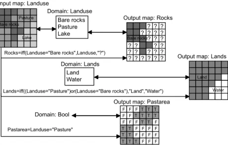
IFF( .. , .. , ..). An IFF function consists of a condition, a then part and an else part. The condition that should be met is written first, followed by the result if the condition is met, and by the result if the condition is not met (Figure 7.2). The result of data retrieval using MapCalc is a new raster map.
Using a Map Calculation formula for data retrieval
In this exercise, raster map Landuseis used for a retrieval operation. This map has a class domain, representing the land use types in the Cochabamba area.
Suppose you are interested in defining the location of the Bare rocksin the area. This can be done by selecting the mapping units with a MapCalcformula.
In words this formula means: If the land use type is Bare rock, then the resulting map (Rocks) will contain the information from the Landusemap (thus class Bare
Figure 7.2: Examples of data retrieval and classification using different MapCalc formulas (see the following exercises for explanation).
•
Type the following formula on the Command linein the Main window:Rocks=iff(Landuse=“Bare rock”,Landuse,“?”)
rock). Or, if the land use is not bare rock, then the pixels in the output map will be classified as undefined, indicated by the “?“ sign. The resulting map Rocksis also a class map and uses the same domain (Landuse) as the input map.
!
MapCalc is not case-sensitive. On the Command line, it makes no difference if you type capitals or small letters.At this stage, only the definition, i.e. the formula to calculate the output map (listed in the Expressiontext box in the Raster Map Definitiondialog box) is saved, but the actual calculation has not yet been performed. When you now open the map, the formula will be calculated.
The map Rocksis displayed on the screen. It only contains one unit:Bare rock. The rest of the map is undefined (?).
It is important to note that this is an example of a rather inefficient way to carry out data retrieval. To get an answer to our question: “Where are the bare rocks” we have created another raster map, which occupies a considerable amount of disk space, and which contains about 90 % undefined values. The information where bare rocks can be found, could be obtained more easily by displaying the polygon map land use with the mask “Bare rock”, as was demonstrated in the previous exercise.
Data retrieval with a Boolean statement
Let us give another example of the use of a MapCalcformula for data retrieval (see Figure 7.2). Suppose we are interested to know the location of the areas with the land use “Grassland”. We will use a so-called Boolean statement. A Boolean statement has only two possibilities: the statement is true (if the condition is met), or it is false (if the condition is not met).
•
Press ↵Enterafter typing the formula. The Raster Map Definitiondialog box is opened. Accept the defaults, and click Define.☞
•
Double-click the raster mapRocksin the Catalog. The Display Options -Raster Mapdialog box is opened. Accept the defaults by clicking OK.☞
•
Close the map window.☞
•
Type the following formula on the Command lineof the Main window:Grass = Landuse = “Grassland”↵
•
The Raster Map Definitiondialog box is opened. As you can see, the sug-gested domain is called: Bool (for Boolean). Click Show.•
Accept the defaults in the Display Options - Raster Mapdialog box by clicking OK. The map is displayed.•
Click the various units to find out what they mean.As you can see the pixels in a raster map with a Bool domain can only be True or False. Undefined pixels in an input map remain undefined in the output map. This is logical, because if you do not know what the land use type is (that is the meaning of the undefined values), you cannot say whether it is grassland or not. A Bool domain thus also allows undefined values. This is different for a similar domain type called Bit. The Bit domain allows only two conditions: 1 (true) or 0 (false), but it doesn’t allow undefined values.
If you use the Bitdomain, undefined values also become 0 (false). It is generally better to use the Booldomain.
Simple reclassification with a MapCalc formula
The previous examples were more intended for data retrieval rather than for
reclassification. No new values were assigned to pixels in the output map. Let us now look at a simple example in which we do want to give the output map a meaning, which is different from the input map.
Suppose, in this example (similar to the one shown in Figure 7.2), that you are interested to differentiate between land and water in the area. The land use units are reclassified into new names, either “Land” or “Water”. These two class names (Land, Water) do not occur in domain Landuse.
The Domainlist box in the Raster Map Definitiondialog box is empty. This is because the program does not know which domain to select, since both the names “Water” and “Land” do not occur in the domain of the input map Landuse. Now there are two options:
- Either you add the items “Water” and “Land” to the domain Landuse, or - you create a new domain with these two class names.
We will select the latter option here. Since “Land” and “Water” are not really land use types, it is better to put them in a separate domain.
•
Close the map window.•
Repeat the calculation: Use the history of the Command line(Arrow Upor open the Command linelist box) to retrieve the calculation on theCommand line.
•
Press Enterand answer the question Overwrite?with Yes. In the Raster Map Definitiondialog box, select domain Bit.•
Display map Grass(now with the Bitdomain), and close the map window when you have finished the exercise.☞
•
Type the following formula on the Command lineof the Main window:Landwater=iff((Landuse=“Lake”)or(Landuse= “Riverbed”),“Water”,“Land”)↵
•
The Raster Map Definitiondialog box is opened.MapCalcformulas are a suitable tool to perform simple reclassifications of class maps, such as the one you just did. However, if you want to assign different values to each of the land use units, the MapCalcformula would become too long and too complicated. Therefore, for more complex reclassifications of raster maps with a class or ID domain, it is easier to store the attributes in a table, and to reclassify the map with the values from the table. This will be demonstrated in the next exercise. Classifying value maps with MapCalc formulas
The final example of the use of MapCalcformulas for (re)classification shows how to classify data from a raster map with domain type value. In this exercise the raster map Dem(Digital Elevation Model) is used. The values in this map represent the altitude of the terrain and range from 2640 to 4500 meters. By performing the next operation a class map with three classes is created (low: ≤3000 meters, moderate: 3000-4000, and high: ≥4000 meters).
This is another way to work with MapCalc; of course you can also type the formula directly on the Command line of the Main window.
•
Click the Create button to the right of the Domainlist box. The Create Domaindialog box is opened.•
Type the Domain NameLandwater. Click OK. Now the Domain Classeditor is opened. Close the Domain Class editor. You are back in the Raster Map Definitiondialog box. Click Show.
•
The Merging domainsdialog box appears, with the question: Add string ‘Water’ to domain ‘Landwater’. Answer with Yes.•
The Merging domainsdialog box appears, with the question: Add string ‘Land’ to domain ‘Landwater’. Answer with Yes.•
The Display Options - Raster Mapdialog box appears. Accept the defaults by clicking OK. The map Landwateris displayed.•
Change the colors of the units: double-click Landin the LayerManagementpane. The Edit Repr. Itemdialog box appears. Change the color to Green; double-click Waterin the Layer Managementpane and change the color to Blue in the Edit Repr. Item.
•
Use the left mouse button to inspect the meaning of the units.•
Close the map window.☞
•
Double-click the MapCalculationitem in the Operation-list. TheMap Calculationdialog box is opened.☞
•
Type the following expression in the text box Expression:iff(Dem<3000,“Low”,iff(Dem<4000,“Moderate”,“High”))
This is called a nested IFF statement: one IFF statement within another.
We can draw the same conclusion as before: MapCalcformulas are suitable for simple classifications. If we want to make more complex classifications, we would need to make many nested IFF statements, which would make the formula too long and too complex. Unlike class and ID maps, there is no possibility to reclassify value maps by an attribute table as value maps cannot have an attribute table.
To solve this problem of complex classifications, we can make use of a special operation, called Slicing. This will be explained in section 7.5.
Summary: Using MapCalc formulas for retrieval and (re)classification
- In this exercise we have seen that it is possible to retrieve information from a map, using a Map calculation formula.
- The expression of a Map calculation formula often has the notation iff(.... , ... , ...) which is called an IFF functionwith conditional, then and else parts.
- The result of a Map calculation formula is a new output raster map. The domain of this output map depends on the contents of the formula. The domain of the output map can either be class, ID or value. A combination of the three is not possible. - If you use a Map calculation formula for the retrieval of one unit in a map, you can
use the same domain for the output map as for the input map, and assign undefined to all other classes.
- Another option for data retrieval using a Map calculation formula is to use a so-called Boolean statement, which can either be true or false.
•
Type Demclassin the text box Output Raster Map.•
Click the Create Domainbutton next to the Domainlist box. The Create Domaindialog box is opened. Type Demclass in the text box Domain Name.•
Accept the defaults by clicking the OK button in the dialog box. The Domain Class editor is opened. Close the Domain Class editor.•
Click Showin the Map Calculationdialog box.•
Accept to add the following items into domain Demclass: Low, Moderateand High.
•
The Display Options - Raster Mapdialog box is opened.•
Accept the defaults and click OK. The map is displayed. Click the units to find out their meaning.•
You can customize the colors in the same way as before.•
Close the map window when you are finished with the exercise.- Data retrieval with a Map calculation formula for vector maps is rather inefficient. The same information can be found easier by displaying the vector map with a mask.
- Data retrieval with a Map calculation formula is required in those situations where you want to use the result map in other calculations.
- MapCalcformulas are a suitable tool for performing simple reclassifications of class maps. More complex reclassifications would require many nested IFF statements.
- Therefore, for more complex reclassifications of raster maps with a class or ID domain, it is easier to store the attributes in a table and to reclassify the map with the values from the table.
- For value maps, the problem of complex classifications can be solved by using a special operation called Slicing.
In this exercise we have only seen some aspects of the Map Calculation functionality. In chapter 8, dealing with overlay operations, there will be a more in-depth discussion on the use of Map calculation.
7.4 Reclassifying a map with attribute data
In section 7.2 you saw that it is possible to display attributes related to a map, without actually generating a new map. In many cases, however, when you want to use such an attribute map in further analysis, it will be necessary to generate a map from the attributes, in an operation called Reclassification, or Attribute Map.
Reclassification involves the (re)assignment of thematic values to the categories of an existing map. In the previous exercise we have seen that for simple reclassification also Map Calculationformulas can be used. If we want to reclassify many classes, the formulas become too complex, and it is better to use attribute tables.
Raster, polygon, segment or point maps with the domain type class, ID, Unique ID, or group can have an attribute table with additional information on the elements in the map. The relationship between the table and the map is provided by their common domain.
When a map is linked to an attribute table, an attribute map can be created based on the columns in the table. In other words, a map linked to an attribute table can be re-classified by its attribute data. The domain type of the column is selected for the new map. The data in the new map represents the information of the column, which can be values, class names or IDs. An example of a reclassification using an attribute table is shown in Figure 7.3.
In this exercise you will first use the polygon map Cityblockto create a new polygon map representing the land use of the city blocks of Cochabamba. The polygon map Cityblockhas an identifier domain; each unit is codified by an ID from 1 to 717. This map has an attribute table, which is also called Cityblock. One Figure 7.3: Example of a reclassification using an attribute table. The
map city block (with a domain ID) is reclassified to the map Landuse (with a class domain) using the column Landuse from the attribute table.
of the columns in this table Landuseshows the dominant land use class for each city block.
The Landuse column is used to reclassify the polygon map and create a polygon map with domain type class representing the land use in the city.
The Attribute Map of Polygon Mapdialog box is opened.
The output map is displayed on the screen.
In chapter 5 (attribute data handling) you have created a table District with information on each district of the city. Now that you have also generated a district map, and as both the map and the table use the same domain (District), you can link the table Districtto the map District.
•
Double-click Attribute Map of Polygon Mapin the Operation-list.☞
•
Select polygon map Cityblockin the list box Polygon Map.•
Select columnLandusein the list box Attribute.•
Type City_Landusein the text box Output Polygon Map.•
Type Dominant land usein the text box Descriptionand click the Showbutton.
•
In the Display Options - Polygon Mapdialog box, accept the defaults by clicking the OKbutton.☞
•
Evaluate the contents of the map by clicking some units.Note that the reference to the city block code is no longer displayed (as was the case in the previous exercise, when we displayed the map Cityblockby its attribute Landuse).
•
Also generate a polygon attribute map District, by using the columnDistrictand the map Cityblock.
☞
•
In the map window, open the Filemenu, select Propertiesand click on the polygon map District. The Polygon Map Propertiessheet appears.•
Click the check box Attribute. Select the table District. Click OKto close the dialog box.•
Open the pixel information window, and drag the polygon maps Cityblock,City_Landuseand Districtto it. Evaluate the contents of the maps and tables while moving with the mouse pointer over the map.
•
Close the map window and the pixel information window.An attribute map can also be made by typing an expression on the Command lineof the Main window. You will now use the Landuseraster map, showing the land use in the entire study area (not just within the city), and the column Landvaluefrom the accompanying table Landuseto reclassify the map.
Summary: Reclassifying a map with attributes
- Vector or raster maps with a class or identifier domain often have an attribute table linked to it.
- The attribute table and the map have the same domain. The table contains columns with attribute information on the units of the map.
- Each of the columns in an attribute table also has a certain domain (either another class domain, an identifier domain, or a value domain).
- You can substitute the classes of the original map by the attribute values from one of the columns in the attribute table. The new map always uses the same domain as the selected attribute column.
- You can make a reclassification using a dialog box, or using the Command line.
•
Position the mouse pointer on the Command lineof the Main window and type the following command:Landvalue=Landuse.Landvalue ↵
•
Click Showin the Raster Map Definitiondialog box.•
Display the map Landvaluewith a Pseudo Representation, and stretch between 100and 750. Close it when finished.7.5 Classifying a value map (Slicing)
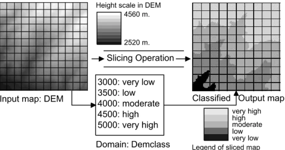
A raster map with the domain type value cannot be reclassified by the method explained in the previous section, since you cannot attach a table to it. Take for example a Digital Elevation Model (DEM). This is a value map which contains a wide range of values. The map DEMin the demo data set, for example, contains values between 2520 and 4560, with a precision of 0.1. Suppose we would like to classify this map into five different height zones. It would require a very large table, with an attribute column containing a lot of repetitive values.
In such a case it is much easier to use a so-called classify table. A classify table contains only the input boundary values and the output class names. In ILWIS the concept of classify tables is applied in theSlicingoperation (Figure 7.4). The classify table in ILWIS is called a Group domain; it contains the input boundary values and output class names.
Ranges of values of the input map are grouped together into one or more output classes. The output map resulting from the Slicingoperation is a map with the domain type group. A domain group should be created beforehand or during the operation using the Slicingdialog box; it lists the upper boundary values of the groups and the group names.
In this exercise the Slicingoperation is performed on the raster map Demin order to group the altitude values (ranging between 2520 to 4560 meter) into five relative altitude classes, shown in Table 7.1.
The raster map Demhas a domain type value in which pixel values refer to the height of the terrain.
Temporary classification for display options
Before the Slicingoperation is demonstrated, it is useful to firstly apply a method, which shows the map, as if it was classified, just by manipulating the maps representation.
The representation can be edited, and the result shown on the screen. Use the
Redrawbutton in the map window, to redraw the map with the updated
representation. This allows you to interactively select the best boundaries for the classification.
Table 7.1: Boundary values and class names for the group domain Demclass. Upper Group name
boundary
3000 <3000 m
3500 3000-3500 m
4000 3500-4000 m
4500 4000-4500 m
5000 4500-5000 m
•
Double-click raster map Demin the Catalog. The Display Options - Raster Mapdialog box is opened. Click OKto display the map.•
In the Layer Managementpane double-click the raster map Demto open theDisplay Options - Raster Mapdialog box again.
•
In the dialog box click the Createbutton next to the Representationlist box. The Create Representationdialog box is opened.•
Type for Representation Name: Demclass2. Accept the other defaults and click OK. The Representation Valueeditor is opened.•
Press the Insert Limitbutton in the toolbar. The Insert Limitdialog box is opened. Enter the limit 3000and select the Color Redand click OK.•
Insert also the other limits shown in the Table 7.1 (3500, 4000, 4500) and select a color for each.•
Click the word Stretchbetween two limits. A list box appears.•
Click once more to open the list box and select Upper. Do this for all ranges in between limits.•
Close the Representation Value editor. You are back in the Display Options - Raster Mapdialog box. Click OK. The map is now displayed as if it was classified.Permanent classification using the slicing operation
Now you will do the actual classification, using the Slicingoperation.
For a group domain, you can enter an upper boundary, a name and a code for each class/group. This domain will be used to slice or classify the raster map Dem. The upper boundaries and group names, shown in the Table 7.1, will be used in this exercise.
When you create a domain group, a representation is also created. It is possible to edit the colors of the output groups/classes from the Domain Group editor, or by opening the representation. To edit the representation:
The Representation Class editor is opened, showing the five groups/classes that are present in the domain with different colors.
•
Expand the Image Processingitem in the Operation-treeand double-click the Slicing operation. The Slicingdialog box is opened.•
Select Dem in the Raster Maplist box.•
Type Classified_Demin the Output Raster Maptext box.•
Type Classified DEMin the Descriptiontext box.•
Click the Create Domainbutton next to the Domainlist box. TheCreate Domaindialog box is opened.•
Type Classified_Demin the Domain nametext box.•
Make sure to select the option Classand the check box Group.•
Click the OKbutton in the Create Domaindialog box. The Domain Groupeditor is opened.
☞
•
Click the Add Itembutton in the toolbar of the editor. The Add Domain Itemdialog box is opened.•
Type 3000in the Upper Boundtext box.•
Type altitude <3000 min the Nametext box. The use of a Codeis optional. It will not be used now.•
Click OK.•
Click the Add Itembutton again, or press the Insert-key of the keyboard to enter the next upper boundary and name.•
Repeat the steps and add the other classes with boundary values, according to Table 7.1: 3500, 4000, 4500and5000.☞
•
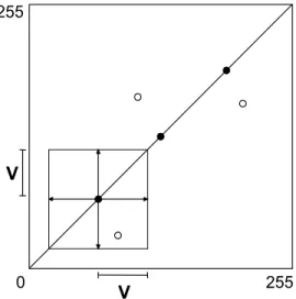
Open the Filemenu in the Domain editor and select Open Representation. You can also click the Open Representationbutton in the toolbar.You can use the Variationcheck box when a random color variation should be used with a certain margin around the straight line between the specified From Colorand
To Colorin the RGB color cube. Subsequently, specify a value between 1 and 255 for the maximum variation allowed. See also Figure 7.5.
To edit a color of a single class, double-click individual items in the Representation Classeditor and either select a pre-defined color, choose a customized color or edit the color of the selected group by changing the amount of Red, Green and Blue.
•
To edit colors of multiple classes (groups), select the first class, press theShift-key and select the last class. Use the right mouse button and select Edit itemsfrom the context-sensitive menu.
•
In the Edit Multiple Itemsdialog box, make sure the option Color Rangeis selected.•
Select two colors (e.g. Whiteand Brown) for the color range between From Color(until 3000) andTo Color(4500-5000) and click OK.☞
Figure 7.5: Two dimensional representation of a color range without variation (solid dots) and a color range with variation (open dots). In the Edit Multiple Items dialog box, you can select the option Variation to use a random color variation with a certain margin (V) in the Red, Green and Blue color cube.
Permanent classification using the CLFY function in MapCalc
A value map can also be classified by typing an expression on the Command lineof the Main window. You will now use this method to classify the landvalue map
Landvalue, generated in the previous exercise. This map shows the value of the land in fictitious monetary values per hectare for each land use type. The values in the map Landvaluerange from 50 to 1000. You will classify this map into three classes: Low(land value lower than 100), Moderate(land value between 100 and 750), and High(land value higher than 750).
The expression has the following structure:
OUTMAP = CLFY(InputMapName, DomainGroup)
in which:
OUTMAP is the name of your output map.
CLFY is the function to classify values according to a domain group.
InputMapName is the name of the input map (domain value map).
DomainGroup is the name of the domain group; it lists the boundaries of the values and the group names for the output map.
•
Close the Representation Classeditor when you are satisfied with the col-ors.•
Close the Domain Groupeditor.•
Click the Showbutton in the Slicingdialog box. The Display Options -Raster Mapdialog box is opened.•
Accept the defaults by clicking OK. The map and the legend are displayed on the screen.•
If you wish, you can change the colors again by double-clicking the word ‘Legend’ in the Layer Managementpane. Press the Redrawbutton in the toolbar of the map window to apply the changes.•
Use the pixel information window to compare the values of the original map (Dem) with the names in the classified map (Classified_Dem).•
Close the pixel information window and the map window.☞
•
Create a group domain Landvalue_class. Add three classes with the boundaries as given above. Use 1000as Upper Boundfor the third class.•
Close the Domain Groupeditor.•
Locate the mouse pointer on the Command lineof the Main window and type the following command:Landvalue_class=CLFY(Landvalue,Landvalue_class)↵
Summary: Classifying a value map
- A value map cannot be reclassified from an attribute table.
- You can make a value map appear classified by creating a new representation value or gradual for it (temporary classification).
- A value map can be permanently classified with the Slicingoperation. The operation requires a group domain. A group domain is a special class domain containing the names of the classes and the boundary values.
- To classify a map, you can also use the CLFYfunction and a group domain. - A group domain can also be used for classifying values in tables (see chapter 5).
•
Click Showin the Raster Map Definitiondialog box.•
Edit the colors if you wish, e.g. Low= Yellow, Moderate= Orange, High= Red.
•
Use the left mouse button in the map window to inspect the result.•
Close the map window when you finished the exercise.7.6 Measurement operations on point maps
In the remaining part of this chapter a new group of operations will be shown: measurement operations. Measurement operations enable you to obtain all kinds of statistical information on vector and/or raster maps. You can do different types of measurement operations, depending on the type of map:
- Points. The number of points in a point map can be calculated, using a
Histogram, or the number of points that fall within the same pixel, using the Point Densityoperation. The distance between points can easily be measured.
- Segments. The number and length of segments (such as drainage lines, roads, or geological faults) can be calculated with the Histogramoperation. The direction of segments can also be calculated. Measurement operations on segments will be treated in section 7.7.
- Polygons. For polygons we can calculate the area of the different units, and the length of the borders around them using the Histogramoperation. This is shown in section 7.8.
- Raster maps. For raster maps we can also calculate histograms. A histogram of a class or ID map is different from the one of a value map. Both types are shown in section 7.9.
Measurement operations on point data
In this section measurement operations dealing with points will be shown: - Calculation of histograms for points
- Calculation of point density within pixels - Calculation of distance between points - Point in polygon calculation
Other statistical operations, which can be performed on point maps, such as Spatial Correlationand Pattern Analysis, will be treated in chapter 11, together with the various point interpolation techniques. There are a series of calculations that can be done with the coordinates of point maps. An overview of these is given in ILWIS Help, topic Point maps, Map calculation special: calculations on point data.
Calculating the number of points
You will first look at the calculation of histograms for point maps. Since there is no appropriate example ready in the demo data set, an operation that will generate points from the geomorphologic polygons (polygon map Geomorphology) will be applied first.
The points you see are the center points of the geomorphologic polygons. The colors are according to the geomorphologic representation (Geomorphology).
The histogram table shows the number of points for each geomorphologic class.
Point density
Another measurement operation for points is Point Density. This operation
calculates the number of points that fall within each pixel. This depends of course on the size of the pixel, which is defined in the georeference. All raster maps (except the satellite images) in the demo data set have the georeference Cochabamba, which has a pixel size of 20 meters. Counting the number of points that fall in each pixel with such a small size, will not make much sense (there will be always only one point in the cell, unless the points are very close). Therefore we will generate another georeference with a much larger pixel size. The same point map (Geompoint) as in the previous exercise will be used.
•
Double-click the Polygons to Pointsoperation in the Operation-list. ThePolygons to Pointsdialog box appears.
•
Select thePolygon MapGeomorphology. Type for theOutput Point Map: Geompoint.•
Type the Description: Center point of geomorphologic polygons.•
Click Show. The point map is calculated and the Display Options - Point Mapdialog box is opened.•
Click OKin the Display Options - Point Mapdialog box. The point map is displayed.☞
•
Close the point map Geompoint.•
Click the point map Geompointwith the right mouse button.•
Select Statistics, Histogramfrom the context-sensitive menu. TheCalculate Histogramdialog box is opened. Since you used context-sensitive menu on the point map Geompoint, this map is already shown as the Input Map. Click Show.
☞
•
In the table window, press the New Graphbutton on the toolbar. The Graphdialog box appears.
•
In the Graphdialog box deselect the X-columncheck box and click OK. TheGraph Optionssheet is opened.
•
On the X-Axistab type for the Axis Text: Geomorphologic unit.•
On the Y-Axis (left)tab change theAxis Textto: Number of pointsand click OKin the Graph Optionssheet. The Bargraph is displayed.•
Close the graph window and the table window.The Point densityoperation is useful, when you are working with point maps that are derived from detailed surveys in which points are measured at close intervals. It may then happen that several points occur within one pixel of the thematic raster maps that you are using. For example, when you are using GPS (Global Positioning Systems), you may take a number of very closely spaced (X,Y,Z) coordinates in the field. An example of an engineering geological application: sample points for soil tests taken in a certain area may be so close to each other that several sample points fall in the same pixel of the soil map that you are using.
Distance between points
With the distance tool distances and directions (angles) can be measured.
•
Click the point map Geompointwith the right mouse button.•
Select Rasterize, Point Densityfrom the context-sensitive menu. The Point Densitydialog box is opened. Since you used the context-sensitive menu on the point map Geompoint, this map is already shown as the input Point Map. Defaults are available for the Point Sizeand the Output Raster Mapname. Accept these defaults.
•
Click the Createbutton next to the Georeferencelist box. The Create GeoReferencedialog box is opened.•
Type for the GeoReference Name: Cochabamba400.•
Type for the Description: Georeference with 400 meter pixel size.•
Change the Pixel Sizeto 400. The number of lines of the raster map will only be 47 and the number of columns 28. Click OK. You return to the Point Densitydialog box. Type the description: Number of points within pixels of 400 meters.•
Click Show. The map is calculated and the Display Options – Raster Mapdialog box appears.
•
Select the RepresentationPseudoand click OK. The map is displayed.•
Press the left mouse button on a few pixels in the map. The points are widely spaced, even with a pixel size of 400 by 400 meters, we only get a maximum of 3 points in 1 pixel.•
Close the map window.☞
•
Open point map Geompoint.•
Click the Measure Distancebutton on the toolbar of the map window, or choose the Measure Distancecommand from the Optionsmenu.•
Click a point of interest somewhere in the map (starting point), hold the left mouse button down, and release the left mouse button at another position (end point). The Distancemessage box appears.The Distancemessage box will state:
From: the XY-coordinate of the point where you started measuring;
To: the XY-coordinate of the point where you ended measuring;
Distance on map: the distance in meters between starting point and end point calculated in a plane;
Azimuth on map: the angle in degrees between starting point and end point related to the grid North;
Ellipsoidal Distance: the distance between starting point and end point calculated over the ellipsoid;
Ellipsoidal Azimuth: the angle in degrees between starting point and end point related to the true North, i.e. direction related to the meridians (as visible in the graticule) of your projection.
Point in Polygon
The last measurement operation that will be shown here is the so-called point in polygon operation, that allows you to rapidly find out in which mapping units the points of a point map are located. This information can be obtained after opening the point map as a table.
The Mapvaluefunction extracts thematic information from any map at a specific location. In this case, information is extracted from polygon map Geology
(Geology.mpa) using the X and Y coordinates of the points in the current point map.
Check the ILWIS Helptopic Table calculation:Special calculations, for other useful functions to calculate with coordinates of a point map.
•
Click OKin the Distancemessage box.•
Close the map window afterwards.☞
•
Click point map Geompointin the Catalogwith the right mouse button and select Open as Tablefrom the context-sensitive menu. The point map is now opened as a table, with two columns: Coordinateand Name. Now it is also possible to use table calculation expressions.•
If you do not see the Command linein the table window first open the Viewmenu and choose Command Line.
•
Type the following formula on the Command lineof the table window:Geology=Mapvalue(Geology.mpa,Coordinate) ↵
☞
•
The Column Propertiesdialog box is opened. Accept the defaults and clickOK. The column Geologynow appears in the table window.
•
Close the table window.Summary: measurement operations on point maps
- A point histogram for a point map with a class or ID domain shows the number of points having the same class or ID.
- A point histogram for a point map with a value domain shows the number of points with the same value, as well as the cumulative number of points (all points with the same value or a smaller value)
- The Point Densityoperation calculates the number of points that fall within the same pixel. It is useful when you want to combine very closely spaced point data with raster maps having a relatively large pixel size.
- With the distance tool distances and directions (angles) can be measured. When the map uses a coordinate system of type projection with an ellipsoid and/or datum also the Ellipsoidal Distance and Ellipsoidal Azimuth are listed in the Distance
message box. When the coordinate system uses a sphere, then the Spherical Distance (distance over the sphere) and the Spherical Azimuth are listed. - A point map can be opened as table.
- The function Mapvalueallows the extraction of thematic information from a map at a specific location.
7.7 Measurement operations on segment maps
You can also calculate histograms of segment maps. In this case, the length of the segments are important, as well as the number of segments. This will be
demonstrated by calculating the length of the geological faults and lineaments of the map Faults.
The segment histogram table shows that there are 17 segments with the code Fault, with a total length of 71 km, and 72 segments with the code Lineament, with a total length of 219 km. In the Statisticspane at the bottom of the table window you can find additional statistical information. You can open the Statisticspane by choosing the Statistics Panecommand from the Viewmenu.
It is also possible to calculate the length of every individual segment. In this case you need to convert the Faultsmap, which has a class domain with two classes, to a unique identifier map. You can do this with the operation UniqueID. This operation calculates unique codes for all points in a point map, segments in a segment map, and polygons in a polygon map.
You will see that each segment now has a different code.
•
In the Catalog, click with the right mouse button on segment map Faults.•
Select Statistics, Histogramfrom the context-sensitive menu. TheCalculate Histogramdialog box is opened.
•
Click Show.☞
•
Close the table window showing the segment histogram.•
Click with the right mouse button on segment map Faults.•
Select Vector Operations, Unique IDfrom the context-sensitive menu. TheUnique IDdialog box is opened.
•
Type Nr. for the Domain Prefix.•
Type the name of the Output Map: Fault_IDand click Show. TheDisplay Optionsdialog box of the segment map is shown.
•
In the Display Options - Segment Mapdialog box select the Infocheck box and select the option Multiple colors, and 15.•
Click OK. The map is displayed.•
Press the left mouse button on some of the segments to check their codes.☞
•
Close the map Fault_IDand open the table Fault-ID.You can now find the most important faults. For example, the faults with a length more than 5 km.
Segment histogram of value maps
A segment histogram calculated for segment maps with a value domain looks slightly different. Take for example the value map Contour.
The histogram table for segment maps with a value domain contains more columns: - Value: the altitude of the contour lines, which have this value code. So the lowest
contour line is 2520 meters and the highest is 4560. - NrSeg: the number of segments occurring for each value.
- NrSegCum: the cumulative number of segments. For each altitude value the num-ber of segments of all the contour lines with a lower or equal altitude is indicated. - Length: the length of all segments with the same value.
- LengthCum: the cumulative length of segments. For each altitude value the total length of all the contour lines with a lower or equal altitude is shown.
•
Locate the mouse pointer on the Command lineof the table window, and type the following formula:Mainfault=(Faults=“Fault”)and(Length>5000)↵
•
The formula can either be true or false. This is called a Boolean statement, and it results in a column with the domain Bool. Click OKin the Column Propertiesdialog box. The new column contains the words True andFalse.
•
Close the table window.•
In the Catalog, double-click segment map Fault_ID. TheDisplay Options - Segment Mapdialog box is opened.•
Select the check box Attribute, select the column Mainfaultand selectWhiteas False Color.
•
Click OK. Only the main faults are shown.•
Close the map window.☞
•
Calculate the histogram of the segment map Contour.☞
•
Close the table window.Segment directions and Rose diagrams
Another useful measurement operation on segment maps, especially for geological applications, is called Segment Direction Density.
The table shows 180 records; one for each degree of the northern part of the geological compass. Record 1 shows the east-west direction. Record 91 shows the north-south direction. It is possible to display the directional data in the form of a
Rose Diagram.
This Rose Diagram shows in which direction faults have the largest length. It is also possible to display the number of segments instead of the length.
Calculating segment density
In many applications it may be useful to know the density of segments within certain units. For example, the drainage density per catchment is often required in hydrologic models, or the density of faults in certain geological units for geological applications. With ILWIS we can generate a segment density map with the operation Segment Density. This operation generates a raster map from a segment map, in which for each pixel the length of certain segments is indicated.
•
In the Catalog, click segment map Faultswith the right mouse button.•
Select Statistics, Direction Histogramfrom the context-sensitive menu. The Segment Direction Histogramdialog box is opened. Since you used the context-sensitive menu on segment map Faults, this map is shown already as the input map. Type the name of the Output Table: Faults.•
Click Show. The table is shown.☞
•
In the table window, open the Graphsmenu and select the Rose Diagramcommand.
•
In the Graphdialog box select Directionfor the X-column, Lengthfor the Y-columnand click OK•
In the Graph Options - Direction x Lengthsheet, select Needleand clickShow.
☞
•
Close the Rose Diagram.•
Open the Graphsmenu again and select the Rose Diagramcommand.•
In the Graphdialog box select Directionfor the X-column, NrLinesfor the Y-columnand click OK•
In the Graph Options - Direction x NrLinessheet, select Needleand clickShow. The rose diagram now shows the number of segments for the different directions.
•
Close the Rose diagram and the table window.This is demonstrated for the segment map Drainage.
The drainage density is now being calculated. After that the Display Options -Raster Mapdialog box is opened.
If the window is sufficiently enlarged, you can see the individual pixels and the red line of the drainage passing over it. The value of the pixel through which a line is passing indicates the length of that line within the pixel. The pixel size of the map is 20 by 20 meters (check this in thePropertiessheet of the raster map). So if the drainage is crossing the pixel in an exact north-south or east-west direction, the length of the line in the pixel is also 20 meters. If the line is oriented in NW-SE or in NE-SW direction, it crosses the pixel diagonally. In that case the length of the segment in the pixel is 28.28 meters (Pythagoras rule). So this is also the maximum possible length of a segment in the pixel, unless you have two segments in the same pixel.
The segment density map by itself is not so useful. It is just showing the length of segments covering each pixel. It is, however, an important input map for calculating the segment density of another thematic map, such as a catchment map. In order to
•
In the Catalogclick with the right mouse button on segment mapDrainage.
•
Select Rasterize, Segment Densityfrom the context-sensitive menu. TheSegment Densitydialog box is opened.
•
Select the check box Maskand type the mask Drainage.•
Select the GeoreferenceCochabamba. Type the Description: Density of drainage lines per pixel.•
Click Show.☞
•
Make sure the RepresentationPseudo is selected.•
Click OK. The map is displayed. You will see a number of colored lines with-in a blue map.•
Zoom in on one of these lines so that you can see only about 20 individual pixels. Click a few pixels to read the values.•
Open the Layersmenu and select Add layer. In the Add Data Layerdialog box select the segment map Drainage and click OK. The Display Options – Segment Mapdialog box appears.•
Select the check box Maskand type Drainagein the text box.•
Select the option Single Colorand choose the color Red.•
Click OK. The segment map Drainageis displayed on top of the drainage density map.•
Close the map window after finishing the exercise.know the drainage density of the different catchments, we need to overlay the raster map of the catchments with the segment density map that we have just created, using the Crossoperation. This will be demonstrated when we deal with the Cross
operation in the next chapter (section 8.4). Summary: measurement operations on segment maps
- A segment histogram for a segment map with a class or ID domain, shows the number and the length of segments having the same class or ID.
- A segment histogram for a segment map with a value domain, shows the number, and the length of segments with the same value, as well as the cumulative number and cumulative length of segments (all segments with the same value or a smaller value).
- A directional histogram shows the number and the length of segments oriented between west and east.
- The data from a directional histogram can be displayed in the form of a Rose Diagram.
- The Segment Densityoperation calculates the length of segments per pixel. It is useful when you want to overlay this map with another thematic raster map (having a class or ID domain) in order to calculate the segment density for each mapping unit, using the Cross operation.
7.8 Measurement operations on polygon maps
For polygon maps we can also calculate histograms. In this case we are most interested in the area of the polygons belonging to the same mapping unit, as well as the number of these polygons. Besides we can also obtain information on the length of the boundary line around each polygon, called the perimeter.
A histogram of the geomorphologic map Geomorphology, with a class domain, will be calculated as an example.
A polygon histogram table contains the following columns:
- NrPol: The number of polygons belonging to each class of the domain.
- Perimeter: The total length of the boundary lines of all polygons belonging to the same class. The values in this column are in meters if the coordinates used in the coordinate system are also in meters (which is nearly always the case).
- Area: The total area of all polygons belonging to the same class. The values in this column are in square meters.
If you need to know the area and the perimeter of individual polygons, you need to convert the map to unique identifiers, with the operation Unique ID, in a similar procedure as explained in the previous section for segment maps. We already have a polygon map with unique IDs in the data set: the city block map Cityblock.
In an ID map, the column showing the number of polygons (NrPol) is obsolete, since all polygons have a unique identifier and therefore each code occurs only once.
•
Click polygon map Geomorphologywith the right mouse button.•
Select Statistics, Histogramfrom the context-sensitive menu. TheCalculate Histogramdialog box is opened.