Identification of strain-rate and thermal sensitive material model with an inverse method

Identification of strain-rate and thermal sensitive material

model with an inverse method

L. Peronia, M. Scapin, M. Peroni

Department of Mechanics, Politecnico di Torino – Corso Duca degli Abruzzi 24, 10129 Torino, Italy

Abstract. This paper describes a numerical inverse methodto extract material strength parameters from the experimental data obtained via mechanical tests at different strain-rates and temperatures. It will be shown that this procedure is particularly useful to analyse experimental results when the stress-strain fields in the specimen cannot be correctly described via analytical models. This commonly happens in specimens with no regular shape, in specimens with a regular shape when some instability phenomena occur (for example the necking phenomena in tensile tests that create a strongly heterogeneous stress-strain fields) or in dynamic tests (where the strain-rate field is not constant due to wave propagation phenomena). Furthermore the developed procedure is useful to take into account thermal phenomena generally affecting high strain-rate tests

due to the adiabatic overheating related to the conversion of plastic work.

of view, anyway it allows to precisely identify the parameters of different material models. This could provide great advantages when high reliability of the material behaviour is necessary. Applicability of this method is particularly indicated for special applications in the field of aerospace engineering, ballistic, crashworthiness studies or particle accelerator technologies, where materials could be submitted to strong plastic deformations at high-strain rate in a wide range of temperature. Thermal softening effect has been investigated in a temperature range between 20°C and 1000°C.

1 Introduction

Aim of this work is to present a combined experimental and numerical technique, based on an inverse approach, to identify work-hardening, strain-rate sensitivity and thermal softening parameters of the material models applied to a dispersion strengthened copper. Stress-strain relationships are usually obtained by fitting experimental data with analytical models. However, the quality of results, obtained with this standard approach, could be affected by geometrical effects (triaxiality of the stress and strain fields) and by the thermo-mechanical coupling in case of high strain-rate. An inverse method is suitable to optimize material strength parameters extracted from experimental results when the stress-strain fields in the specimen are not correctly described by the analytical models. This commonly happens in specimens with no regular shape, in specimens with regular shape when some instability phenomena occur (for example the necking phenomena in

e-mail : [email protected]

tensile tests that creates a strongly heterogeneous stress-strain fields) or in dynamic tests (where the strain-rate field is not constant due to wave propagation phenomena).

The inverse method described in this paper relies on three main steps:

- experimental compressive and tensile tests performed at different speeds (from quasi-static loading to high strain-rate) and different temperatures (from 20 °C to 1000 °C);

- experimental results fitted with analytical models in order to obtain reference material strength parameters that can be used as starting trial points in inverse method optimization;

- optimization of material strength parameters via numerical FEM simulations of the experimental tests.

It is important to remark that an effective material characterization must count on a specified analytical model from which depend the number of strength parameters and types of experimental tests to be performed. For this reason it is very important that experimental test and numerical modelling go hand in hand in order to avoid both an inadequate and an overflowing number of data. Next paragraph describes the analytical models used for this study.

2 Material model

Elasto-plastic strain-rate and thermal sensitive models such those proposed by Johnson and Cook (J-C) [1] and Cowper-Symonds (C-S), are the most used to describe work-hardening, thermal softening and strain-rate sensitivity behaviour of ductile materials. In FEM codes there are also more complex models, such as Zerilli Armstrong model, but they request the identification of a larger set of parameters.

The commercial FEM code LS-DYNA® [2], used for numerical simulations, in addition, allows the implementation of user-defined routines for material models. In this work a user-defined J-C model is used instead the LS-DYNA® standard one, in order to overcome some limits (e.g., the solution of implicit axisymmetric models) and save additional output variables (e.g., strain-rate and temperature). The J-C material model expresses the flow stress as

(

)

( )

T C

B

A n

y

*

0

pl 1 ln 1−

  

  

+ +

=

ε ε ε

σ

& &

(1)

In (1), A is the elastic limit strength, B and n are the work hardening parameters, C and ε&0 are the

strain-rate sensitivity parameters and T* and m are the thermal softening parameters.

Thermal softening is essentially due to heat conversion of plastic work occurring at high strain-rate deformations. Forε&≥102 s-1 thermal diffusion can be neglected and thermal softening can be evaluated under adiabatic assumption. Given this last hypothesis and the further assumption of uniform stress, strain and temperature fields, the material temperature can be analytically computed as a function of plastic work as shown in expression (2). Actually temperature increase is not uniform but grows up in the material with a distribution corresponding to plastic work (as it will be confirmed via numerical simulations).

(

)

ρ

β ε

d T C

T T

p

p

r+ _⋅ ⋅ ⋅

=

_∫

0

,

,&

2 Experimental tests

Object of this study is a dispersion strengthened copper, known by the trade name GLIDCOP, that finds several applications in particle accelerator technology, where problems of thermal management combined with structural requirements play a key role [5]. So, it is very important underlying that due to the extreme working condition in which the material could operate, it is fundamental characterize it in a wide range both in strain-rate and in temperature. Glidcop has material properties similar to OFE copper, such as thermal and electrical conductivity. Unlike OFE Cu, however, Glidcop has yield and ultimate strengths equivalent to those of mild-carbon steel, making it a good structural material. Besides, it keeps good mechanical properties also at high temperatures.

Fig. 1. Facilities for the high strain-rate tests: (a,b) Hopkinson bar; (c) Taylor test (gasgun).

Since the material model is uncoupled in strain, strain-rate and temperature effects, the experimental test are managed exchanging one parameter at a time. So, experimental compressive and tensile tests were performed at different speeds (10-3, 10-1, 10, 103 s-1 at 20 °C) and different temperatures (20, 100, 200, 300, 400, 500, 600, 700, 850 and 1000°C at 10-3 s-1).

Striker bar Output bar Input bar

Strain transducer

Space

T

im

e

Transmitted waves

Reflected waves

Incident wave

Specimen

Fig. 2. Scheme of the Hopkinson tensile bar set up and the specimen used in tensile test.

Quasi-static loading condition was obtained via general purpose hydraulic testing machine while medium strain-rates tests were performed with pneumatic equipments [6]. High strain-rates compressive tests were carried out with a Hopkinson pressure bar [7] while tensile tests were performed via a customized direct set up (Figure 1.a) developed from the solution proposed in [8]. Figure 2 shows a scheme of the developed equipment with a detail of specimen clamping system and the Lagrangian wave propagation diagram during a test.

(b) (a)

(c)

M10

Lu R=5

In this SHPB tensile setup, the striker bar and the input bar are hollow cylinders while the output bar (that is a classical cylindrical bar) is coaxial with the input bar. The test starts generating a compression pulse in the input bar because of the impact of the tubular striker bar. When the compression pulse reaches the opposite extremity of the input bar applies a tensile stress on a plate that is fixed on one threaded specimen end. In this way the compression pulse applies a tensile stress also to the specimen carrying out the tensile test.

Fig. 3. (a) Facilities for the temperature tests; (b) Picture of the compressive test performed at 850 °C and (c) the correlated image from the thermo-camera.

The experimental tests at different temperatures were performed (Figure 3.a) on an electromechanical machine using an induction heater with feedback on a thermo-camera (for tests at temperature lower than 400°C) and an infrared sensor (for tests at temperature greater than 400° C). In Figure 3.b it is shown a picture of the compressive test performed at 850 °C and the correlated image from the thermo-camera. Finally, in order to verify the extracted material parameters and investigate high dynamic load conditions, it was set up the Taylor test at different speeds (between 100 and 400 m/s) using a Light Gas Gun (Figure 1.c).

0 0.05 0.1 0.15 0.2

0 100 200 300 400 500 600

True plastic strain (-)

T

ru

e

s

tr

e

s

s

(

M

P

a

)

strain-rate 10-3 s-1 strain-rate 10-1 s-1 strain-rate 101 s-1 strain-rate 103 s-1

10-3 10-1 101 103

0.9 1 1.1 1.2 1.3

Strain-rate (s-1)

S

tr

a

in

-r

a

te

c

o

e

ff

ic

ie

n

t

Experimental test J-C fit

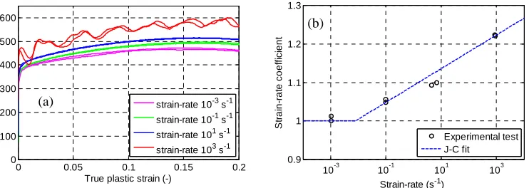
Fig. 4. (a) Experimental true stress-true plastic strain curves at different strain-rates in the tensile tests; (b) J-C strain-rate coefficient.

Figure 4.a and 5.a show the true stress-true plastic strain curves, respectively, at different strain-rate obtained in tensile tests and at different temperatures obtained in compressive tests. Figure 4.b and 5.b display, respectively, the strain-rate and temperature coefficients extracted via analytical method for the J-C model (expression 1). The reference values obtained in this way can be optimized via numerical procedure as described in the next paragraph. The true stress-true plastic strain curves are obtained from the original experimental data (force-displacement curves) considering a specimen with gage length of 10 mm and diameter of 5 mm for the tensile tests and a specimen with length of 10 mm and diameter of 6 mm for the compression tests.

(b)

(a)

(a) (b) (c) 850.0

0 0.05 0.1 0.15 0.2 0

100 200 300 400 500

True plastic strain (-)

T

ru

e

s

tr

e

s

s

(

M

P

a

)

1000°C 850°C 700°C 600°C 500°C 400°C 300°C 200°C 100°C 20°C

373 473 573 673 773 873 973 1123 1273 0

0.2 0.4 0.6 0.8 1

T

e

m

p

e

ra

tu

re

c

o

e

ff

ic

ie

n

t

Temperature (K)

Experimental test J-C fit

Fig. 5. (a) Experimental true stress-true plastic strain curves at different temperatures in the compressive tests; (b) J-C thermal coefficient.

3 Numerical Inverse Method

Reference parameters of the material, obtained by fitting experimental curves with analytical J-C, have been implemented into a FEM code in order to numerically simulate all the experimental tests previously performed. FEM models have been developed with the commercial code LS-DYNA® [2] which includes implicit and explicit solver with thermo-mechanical and highly non-linear capabilities. In order to reduce CPU time and to staunchly reproduce experimental tests, FEM models only include the specimen to which is applied a load history directly registered from testing equipments. In particular, for high strain-rate tests, the load applied to the specimen by input and output bars of the SHPB, is reconstructed and implemented into the FEM model with the elaboration techniques proposed in [8].

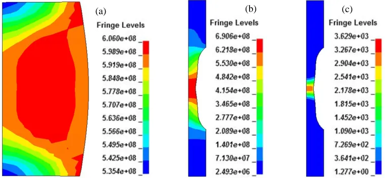
Fig. 6. Von Mises stress (Pa) distribution in a compressive specimen (a) and in a tensile one (b). In (c) the strainrate (s-1_{) distribution in a test nominally at 1000 s}-1_.

Numerical simulations provided results having significant discrepancy with respect to the experimental data. In fact, reference parameters of the material have been obtained from experimental data with a standard fit relying on the following assumptions:

(a) (b) (c)

(a)

- uniaxial stress and strain inside the specimen. Actually, three-axial stress and strain fields inside the specimen are provoked by the friction between specimen and testing equipment during compressive tests (Figure 6.a, 7) and by the necking of the specimen during tensile tests (Figure 6.b); - constant strain-rate inside the specimen. Actually the strain rate is not constant and uniform during dynamic tests (Figure 6.c), thus influencing stain-rate sensitivity parameters;

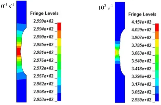
- uniform temperature inside the specimen. Actually the temperature has a certain distribution proportional to the distribution of plastic deformation inside the specimen, and the effect is even higher for dynamic tests (Figure 8, 9). This should be considered to identify thermal softening parameters.

Fig. 7. A sequence of steps of experimental test performed with SHPB filmed with high velocity camera (20.000 fps): due to the friction between specimen and testing equipment the deformation is not uniform (barrelling). The sequence is used to validate the numerical simulations friction model.

Fig. 8. Temperature distribution (°C) in a compression specimen (experimental)

Fig. 9. Temperature distribution (K) in a tensile specimen at two different strain-rates.

With the intention of remove these assumptions a numerical optimization of the parameters is needed. Aim of the inverse method is the determination of selected set of unknown parameters in a numerical model in order to correctly reproduce experimental tests with FEM calculations. In particular, in this work, the comparison is done in terms of force-displacement curves. Core of this

10-1 s-1 ₁₀3

s-1

60.0

procedure consists of iteratively solve numerical simulations having the experimental curves as objective functions, starting from trial values of the parameters obtained from a standard analytical optimization method. Optimization of the parameters has been performed with dedicated algorithm included in the software LS-OPT®. Numerical simulations include all experimental tests performed at different speeds and temperatures. The optimization algorithm works with a multiple objective function, this requires to run simultaneously all the simulations relative to a specific set of parameters that must be optimized.

It is important to remark that in J-C model, work-hardening, thermal softening and strain-rate effects are linearly independent. This allows to separately optimize each set of parameters. So, a first optimization is done in order to extract the strain dependence (A, B and n of the expression 1) and the thermal coefficients (m and T* of the expression 1) based on the static test at different temperatures. Then a second optimization is done to extract the strain-rate coefficients (C and ε&₀of the expression 1) based on the dynamic tests. This aspect is particularly important because if it is true that the material model decouples the various effects, actually in the experimental dynamic tests the work to heat conversion couples them again and makes them difficult separable, if (as happens in this procedure) at least one of the effects is not already known.

0 0.5 1 1.5 2 2.5 3 3.5

0 5 10 15 20 25 30

Stroke (mm)

F

o

rc

e

(

k

N

)

strain-rate 10-3 s-1 strain-rate 10-1 s-1 strain-rate 101 s-1 strain-rate 103 s-1 numerical fit

0 0.5 1 1.5 2 2.5 3

0 2 4 6 8 10 12

Stroke (m)

F

o

rc

e

(

k

N

)

strain-rate 10-3 s-1 strain-rate 10-1 s-1 strain-rate 101 s-1 strain-rate 103 s-1 numerical fit

Fig. 10. Results of numerical simulation after the optimization procedure: (a) compression, (b) tension.

In dynamic tests, in fact, the adiabaticity causes the material to warm up much during the test producing a softening of the material in contrast with the dynamic strain hardening produced by strain-rate. In the past this fact created many interpretation problems of the results of such tests: in the early stages of test the strain-rate hardening effect prevails and loads increase; as the specimen is deformed (especially in very ductile materials) it warms and decreases its resistance. The result is a tension-deformation curve which differs in shape from the static, while in model (1) the shape is dictated only from the strain hardening and this seems an obvious contradiction. The contradiction disappears when the assumption of constancy of the dynamic and thermal multiplicative factors is removed. Results of the numerical optimization are shown in Figure 10 for the tests at different strain-rates. Figures 6, 9 show some examples of numerical simulation results at the end of the optimization procedure.

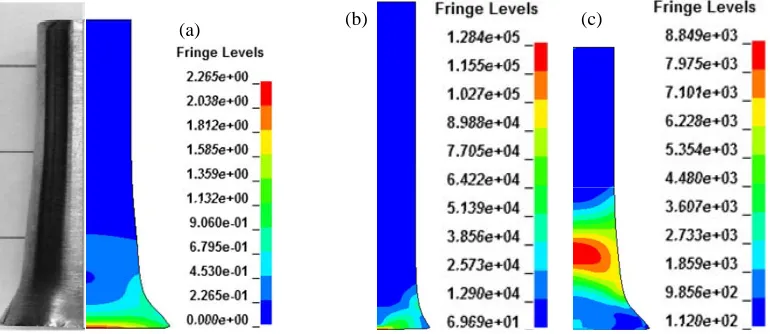
Figure 11 instead shows some results of Taylor test: this test extremely simple in principle, allows to reach high levels of strain-rate if the specimen is launched with a gasgun at speeds exceeding 100 m/s. Unfortunately, the deformation, stress, strain-rate and temperature fields are far from uniform. The procedure presented above could also cover these tests in the global procedure of optimization of model parameters in order to extend the level of strain-rate confidence.

4 Conclusions

A combined experimental and numerical technique, based on an inverse approach, for material model identification was fully developed and applied to a dispersion strengthened copper.

Once chosen the analytical model used to describe material behaviour (J-C was employed), several experimental tensile and compressive tests were performed at different speeds and different temperatures. Reference parameters of the material have been obtained by fitting experimental data with the analytical models. Finally material parameters have been optimized through an inverse numerical procedure: FEM simulations of all experimental tests have been performed and parameters were iteratively changed in order to reproduce the experimental curves.

The procedure described in this paper is generally valid for the identification of every material models, anyway the method must be adapted on the basis of the choice of the analytical model used as a reference. J-C model allowed, in this case, to independently optimize work-hardening, thermal softening and strain-rate sensitivity parameters limiting the complexity of thermo-mechanical characterization of the material.

The inverse method presented, requires strong effort both from experimental and numerical point of view, anyway it allows to precisely identify the parameters of different material models. This could provide great advantages when high reliability of the material behaviour is necessary. Applicability of this method is particularly indicated for special applications in the field of aerospace engineering, ballistic, crashworthiness studies or particle accelerator technologies, where materials could be submitted to strong plastic deformations at high-strain rate in a wide range of temperature. Thermal softening effect has been investigated in a temperature range between 20°C and 1000°C.

References

1. Johnson, G. R., Cook, W. A., A constitutive model and data for metals subjected to large strains, high strain rates and high temperatures, 7th Int.Symposium on Ballistic, (1983), pp. 541-547 2. Gladman, B. et al. LS-DYNA® Keywords user’s manual (2007) Volume 1, LSTC

3. Macdougall, D., Exp. Mech., (2000), Vol. 40, pp. 298-306

4. Hodowany, J., Ravichandram, G., Rosakis, A. J., Rosakis, P., Exp. Mech., (2000), Vol. 40, pp. 113-123

5. R. Valdiviez, D. Schrage, F. Martinez, W. Clark, The use of dispersion strengthened copper in accelerator design, XX International Linac Coference, Monterey, California

6. Peroni, L., Peroni, M., Meccanica, Volume 43 (2008), pp. 225-236

7. Peroni, M., Experimental methods for material characterization at high strain-rate: analytical and numerical improvements, (2008), PhD Thesis, Politecnico di Torino

8. Newby, J. R., ASM Handbook, Metals Handbook. Mechanical testing Vol. 8

(b) (c)