A computer controlled random wave generator

A COIVIPUTER CONTROLLED

GENERATOR

A THESIS SUBMITTED IN FULFILMENT OF THE REQUIREMENT FOR THE DEGREE OF

MASTER OF ENGINEERING IN MECHANICAL ENGINEERING

BY

VINCENT ROUILLARD

DEPARTMENT OF MECHANICAL ENGINEERING FOOTSCRAY INSTITUTE OF TECHNOLOGY

VICTORIA UNIVERSITY OF TECHNOLOGY VICTORIA, AUSTRALIA.

ABSTRACT

Simulation of ocean wave processes and model studies related to marine

technology are areas of increasing economic and environmental importance. Sophisticated laboratory facilities are needed to model ocean wave

phenomena under controlled conditions. This thesis describes the techniques and principles employed in the design, commissioning and

evaluation of a computer controlled random wave generation facility devised to accurately simulate spectral wave models.

A discussion on the classification of ocean waves is presented together with a review of classical wave theories and their range of application. The treatment of water waves as a random process is presented along with an outline of current spectral analysis techniques. Statistical properties of random waves are considered and a description of various mathematical

spectral models used to represent ocean waves is given.

Various designs and random wave generation techniques employed in existing laboratory wave generators are critically reviewed. A detailed description of the design of the wave generator, wave absorbers and wave probe is

presented. Computer software developed for managing the wave generator was principally designed to control the wave maker motion and carry out

spectral and statistical analyses of recorded wave data.

Experiments aimed at evaluating the characteristics of the wave generator and ancillary equipment are outlined. Both the static and dynamic

TABLE OF CONTENTS

PAGE

Acknowledgements iv

List of figures v

List of tables vii

1. Introduction 1 1.1 Background 1 1.2 Aim and Significance 2

2. i?eview of Classical Wave Theories 3

2.1 Classification of Ocean Waves 3

2.2 Development of Classical Wave Theories 4

2.3 Small Amplitude Wave Theory 11 2.4 Finite Amplitude Wave Theory 18

2.5 Stoke's Wave Theory 22

2.6 Cnoidal Wave Theory 24

2.7 Solitary Wave Theory 24

2.8 Stream Function Wave Theory 24

2.9 Wave Superposition 25

3. Statistical Analysis of Ocean Waves 33 3.1 Spectral Analysis of Random Processes 33

3.2 Spectral Models of Ocean Waves 39

3.3 Distribution of Water Surface Elevation 44

3.4 Distribution of Surface Elevation Maxima 46

TABLE OF CONTENTS (cont'd)

4. Wave Generation Equipment and Software 56

U.l Review of Wave Generators 56

4.2 Design of Wave Generator 62

4.3 Wave Probe 73

4.4 Wave Absorbers 75

4.5 Control System 77

4.6 Software Development 78

4.6.1 Wave Probe Calibration 78

4.6.2 Reflection Evaluation and Regular Wave Generation 79

4.6.3 Random Wave Generation 80

4.6.4 System Frequency Response Measurement 88

4.6.5 Statistical Analysis 89

5. Results and Discussion 93

5.1 Experiments 93 5.2 Wave Probe Characteristics 93

5.3 Wave Energy Absorber Characteristics 96

5.4 System Frequency Response Evaluation 97

5.5 Comparison of Open and Closed-loop Performance 106

5.6 Generation of Single Peak Spectral Models 114

5.7 Generation of Double Peak Spectral Models 123

6. Conclusions 129

Bibliography 130

Appendix A. Further Theoretical Relationships for the Wallops

Spectrum 136

ACKNOWLEDGMENTS

I wish to express my deep appreciation to Dr. G.T. Lleonart, who initiated

and supervised this study, for his valuable guidance and helpful

suggestions. My gratitude extends to Mr. R. Juniper, Dr. M.A. Sek and Mr.

J. McLeod for their constructive advice. My thanks also go to the

technical staff of the Department of Mechanical Engineering and the Fluid

Dynamics Laboratory who contributed in the construction of the wave

generation facility.

I would finally like to thank the secretarial staff of the Department of

LIST OF FIGURES

2.1 Estimation of the distribution of wave energy. 2.2 Conservation of mass.

2.3 Rotation of a fluid particle.

2.4 External forces acting on a fluid element. 2.5 Schematic diagram of a small amplitude wave. 2.6 Effects of water depth on fluid particle paths. 2.7 Classification of wave theories.

2.8 Stationary finite amplitude wave. 2.9 Second order Stoke's wave.

2.10 Illustration of various wave profiles.

2.11 Polar representation of common harmonics of arbitrary phase. 2.12 Nodes and antinodes of wave envelope.

3.1 Linear system input-output relationships.

3.2 Variation of the water surface elevation maxima with spectral width parameter.

3.3 Narrow band random process. 3.4 Definition of wave heights. 3.5 Variation of Hj^,^/ 2MQ.

4.1 Some types of wave makers.

4.2 Schematic of wave generation facility. 4.3 Wave maker support arrangement.

4.4 Wave maker dimensions. 4.5 Wave maker plunger. 4.6 Wave maker arrangement. 4.7 Wave generator arrangement.

4.8 Force excitation of A frame model for FEA. 4.9 Deflection response of A frame.

4.10 Displacement excitation of pivot beam for FEA. 4.11 Displacement response of pivot beam.

4.12 Electro-hydraulic wave generator system. 4.13 Wave probe.

4.14 Wave energy absorbers.

LIST OF FIGURES (cont'd)

4.16 Illustration of control method for random wave generation. 4.17 Random wave generation control flow chart.

4.18 On-line menu for random wave generation.

4.19 Signal generation and acquisition method for random wave generation.

4.20 Spectral moments computation method.

5.1 Wave probe static calibration curves. 5.2 Time response characteristics of wave probe. 5.3 Stoke's breaking wave profile.

5.4 Breaking wave measurement.

5.5 Amplitude reflection characteristics of wave tank. 5.6 Definition of single and dual stage systems.

5.7 Single and dual stage system frequency response estimates. 5.8 Variation of system frequency response with wave probe

location.

5.9 Variation of system frequency response with input signal level 5.10 Open-loop spectral estimates.

5.11 Closed-loop spectral estimates.

5.12 History of measured spectral estimates. 5.13 Control system recovery.

5.14 Single peak target spectra. 5.15 Command signal distribution. 5.16 Single peak spectrum - experiment 1. 5.17 Single peak spectrum - experiment 2. 5.18 Single peak spectrum - experiment 3. 5.19 Single peak spectrum - experiment 4. 5.20 Double peak spectrum - experiment 5. 5.21 Double peak target spectra.

5.22 Double peak spectrum - experiment 1. 5.23 Double peak spectrum - experiment 2. 5.24 Double peak spectrum - experiment 3.

LIST OF TABLES

5.1 Experimental conditions - single peak spectrum. 5.2 Statistical results - single peak spectrum.

5.3 Experimental conditions - double peak spectrum.

1. INTRODUCTION

1.1. Backgrotind.

Oceans are a major source of minerals, energy and food and constitute an essential means of communication, distribution and transport. The motions in the upper ocean provide the means for the exchange of matter, momentum and energy between the atmosphere and the underlying ocean. These

exchanges produce the general circulation pattern in the oceans and at the same time form one of the most important factors in the worldwide

distribution of climate.

Successful ventures in the marine environment, such as the design and construction of ships, structures, diving, dredging, drilling and towing equipment as well as communication equipment require a wide range of information and professional advice on the behaviour of the oceans.

Even to the casual observer, the random nature and continually changing condition of the ocean surface is evident. Waves of different lengths travelling at different speeds combine and recombine to form constantly changing patterns. For a long time it was thought that this apparently chaotic process was beyond adequate mathematical description. In comparatively recent times, the development of an approach based on the combination of statistics, Fourier analysis and hydrodynamics promises a better understanding of real sea conditions. Statistical theories have been used to determine stable parameters for describing random sea states, Fourier analysis was then employed to separate the random process into harmonic components which can be analysed using classical theories of wave motion.

laboratory where the analysis of these motions and the development of a coherent theory can be undertaken. It is only by drawing these

considerations together in a consistent manner that the nature of ocean wave motion may be better understood.

1.2. Alms and Significance.

There is a need for wave generators which can be readily and accurately programmed to undertake experimental studies on wave phenomena and scale

modelling of offshore structures, mooring systems, breakwaters, beaches and other marine engineering systems. Such a laboratory facility would provide

a tool for deepening our understanding of the basic design and physical processes involved.

With the advent of digital computers and electronically controlled servo-mechanisms, wave generators can be controlled more accurately and

reliably. Furthermore, with digital computers, optimal control techniques such as feedback compensation in the frequency domain, are more easily

implemented.

The principal aim of this work is to design and commission a computer

2. REVIEW OF CLASSICAL WAVE THEORIES

2.1. Classification of Ocean Waves,

In this chapter the classical theories for unsteady free surface flow

subjected to gravitational forces are reviewed. Such motions are called water waves. They are also called gravity waves. From a physical

standpoint there are a great multiplicity of water waves which range from tsunami waves generated by earthquakes to seiches in harbours; from tidal

bores in estuaries to waves generated by wind in the oceans.

Water wave motions are of such diversity and complexity that classification is far from simple. One method of classifying ocean waves is by estimating

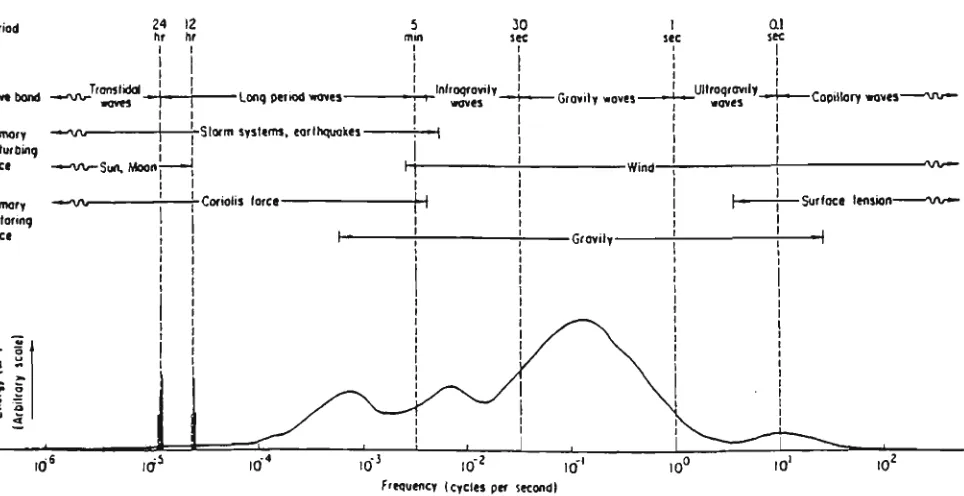
the relative energy content at various wave periods. Figure 2.1, after Kinsman (1965), shows that a large amount of energy is associated with

gravity waves. These waves, with periods ranging from 1 to 30 seconds, are of primary concern.

Period

ibon) -».W/- Copillory w j v * * — - w / ^

PfimorY dhlurbing (orc(

Primarif - ~ w restonnq

lorct

la 10" 10' 10"

Fttquencv (cycles per secondl

10"

Figure 2.1. Estimation of the distribution of ocean wave energy. After Kinsman (1965)

-Gravity waves in the ocean are further distinguished according to the

(i) Sea - waves created by direct action of the wind on the ocean surface.

(ii) Swell - waves caused by distant meteorological disturbances which have spread from the generating area and are no longer subjected to significant wind action.

Seas generally consist of steeper, higher frequency waves of shorter wavelengths and are more chaotic than swells. Swells persist after the source of disturbance has disappeared and maintain a constant direction so long as deep water conditions prevail. Sea waves, caused by local wind, are often superimposed on swells and interactions between the two can cause unpredictably high waves.

2.2. Development of Classical Wave Theories.

Water wave theories may generally be classified in two main groups. These are the small amplitude wave theories and the long wave theories. The small amplitude wave theories cover the linearised solutions for

infinitesimal amplitude waves as well as power series in terms of the wave height to wavelength ratio for finite amplitude waves. Long waves theories

include the numerical methods of solutions generally used for solving

nonlinear long wave equations. The two groups encompass cases exhibiting features of both groups. For instance, cnoidal and solitary waves are

considered as special cases of the long wave theories since they are nonlinear shallow water waves.

Water waves have traditionally been treated as the combination of many

different waves of various amplitudes, wavelengths and shapes. In order to omit most of the complicating factors, classical wave theories assume the waves to be periodic and uniform. Classical wave theories are developed by approximating solutions to the differential equations describing the

kinematic and dynamic conditions under certain specific boundary conditions.

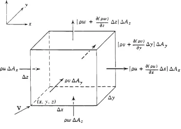
z

A

L\pw + ^1^£^\^A,

puAAx

po-^^ Ay] AAy

•^{pu+^Jp.Ax]AA:c _ox

pw

AA-Figure 2.2. Conservation of mass.

The law of conservation of mass is expressed by

5 (pti.V) S(pu)AxAA.y ^ 5 (pv)LytiA ^ 5 (pw)t^hA^ 5t Sx Sy Sz

(2.1)

where p is the fluid density and u, v and w are the velocities in the X, y and z directions respectively.

Since hV =• LA^ =• AA =• AA^, equation (2.1) reduces to

Sp St

- ^(P"^ + 5(pv; ^ S(pw) 5x Sy

(2.2) Sz

If it is assumed that the fluid is incompressible, the continuity equation may be written as

1 H

+ .§Z +

=

5x Sy Sz

(2.3)

be used to solve problems. Most of these methods result from the existence of a special function known as the velocity potential. In general, the

motion of the fluid particles may be considered irrotational when the velocity gradient is small, such as in periodic gravity waves.

Mathematical simplification is achieved in the treatment of fluid flow

problems if the fluid in considered to be irrotational.

dw Ax dx 2

/ /

[(" ^ fe f ) - (" - fe f )]-'

u + du Az _{dz 2}

/

r

-0 _{x.z) I u}

"4*

Ax

V^'

/

f Element at Ume t + At

/

/ dw w + -r— dx 2 4£

T

/

,w +

u — du Az _{dz 2}

dw Ax dx 2

i

)-(-t¥)h

Element at time t

- ^ ^ X

Figure 2.3. Rotation of a fluid particle.

For simplicity, the motion of a two-dimensional rectangular fluid particle

with its centre of mass at (x,z) is considered as shown in figure 2.3.

After a short time interval At, the element is subjected to a small

deformation. From the geometrical configuration of figure 2.3, the mean

velocities of the fluid particle faces, for planes parallel to the x axis,

are

u - 5u Az

Sz 2

and _{u +} 5u Az

Sz 2

and for planes parallel to the z axis,

w - 6w A x

5x 2 and w +

Sw A x

(2.5) Sx 2

In a time interval At, the difference in the velocities of opposing

planes will result in the deformation of the fluid particle as shown by the dotted line in figure 2.3. The mean rate of change of the angles a and 0 may then be written as

Aa

At

fv + i2. ^ 1 - (v - ii: Ax)

(2.6)

and

At u +

6u Az\ _ (u _ 6u. A £ \

Sz 2 I \ Sz 2 I At/(Az At; = - iiL Sz

(2.7)

where anticlockwise rotations are considered positive.

The mean angular velocity, Qy» °^ ^^^ fluid particle in the x-z plane is therefore

Qi 2

Sw _ ^u_

5x Sz

(2.8)

If three dimensional flow is considered, the remaining two components of the rotational vector are given by

a

Sy Sv

Sx in the x - y plane

(2.9)

and

% , 1

Sz

Sw

Syj in the z - y plane

(2.10)

The flow is rotational if Qj^ = 0.2 " ^3 °^

Sw ^ ^ Sx Sz

Sw ^ 5u^

Sx Sz and Sx Sz ^ ^ ^

It can be stipulated that there exists a velocity potential represented by the scalar function i(x,y,z,t) which, by definition, satisfies

u - i i , v = ii and v - i l (^•^2> Sx Sy Sz

If it is assumed that the velocity potential has continuous derivatives, then

A (§1\ = _1 / i l l o r iM - 5w; (2.13) Su „

Sz

5x

Sw _

Sy Sw Sx

Su Sy

Sv Sz

Sz \SxJ Sx \ Sz

Al§^\ §.(§!] or 5v ^ 5u (2.14) Sx \ Sy j Sy \ Sx

A(§±\^A(§±\ or ii? - 5v (2.15) Sy \SzJ Sz \Sy

which are the conditions for irrotational flow. Consequently, for irrotational flow of an incompressible fluid, the continuity equation reduces to

S^§ + i f i ^ _ 5 ^ „ Q (2.16)

Sx^ Sy^ Sz^

which is known as the Laplace equation.

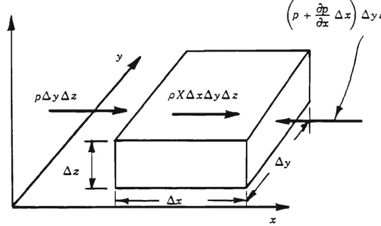
The dynamical equations of motion are derived by considering the forces acting on an elemental mass of fluid. By Newton's second law of motion, the net sum of the external forces acting on a mass must be equal to the rate of change of the linear momentum.

By considering an elemental mass of frictionless fluid in rectangular Cartesian coordinates, as shown in figure 2.4, the sum of the forces in the X direction is

pAyAz - Ip + l£ Ax] AyAz + XpAxAyAz - pAzAyAz • ~ (2.17)

p + ^ Az) AyAz

Figure 2.4. External forces acting on a fluid element.

Equation (2.17) reduces to the equation of motion for a frictionless fluid in the x direction :

^ - X dt

Similarly

dv ^ Y dt

^ . z

dt

_ 1_ Sp p Sx

-

LAt

p Sz

(2.18)

- equation of motion in the y direction

- equation of motion in the z direction

(2.19)

(2.20)

Alternatively, the equations of motion in the x, y and z directions may be written as

J f - i . i £ - . ^ - i H . + u ^ + v i H + viH

p 5x dt St Sx Sy Sz (2.21)

p 57 dt St Sx Sy Sz (2.22)

Z - AAL ~ ^ ~ § E + U^ + V^ + W^

p Sx dt St Sx Sy Sz (2.23)

X ^ 0 , Y s O and Z ^ - g ^ - ^^^z) (2.24) Sz

Under the assumption that the motion is irrotational and from the

definition of the velocity potential, the continuity equations become

- AiE = -A-1 + u^ + v^ + w^ (2-2^)

p Sx 5x51 5x 5x 5x

-AlR- -Ah + u^+ v^ + w^ (^-^^^

p Sy SySt Sy Sy Sy

_ S(gz) _ 1 Sp ^ _ sh ^ „5u ^ ^,5v ^ ^^Sw (2.27) Sz p Sz SzSt Sz Sz Sz

If the fluid density is assumed to be uniform, equations (2.25), (2.26) and (2.27) may be written as

A.(-il+l (u2 + v2 + z^) + ^ ] = 0 (2.28) Sx \ St 2 p I

Sy \ St 2 ' pj

_ i _ ( - i l + l . C u ^ + v^ + z^) + P . + gz) = 0 (2-30)

Sx \ St 2 P I

Integrating and combining equations (2.28), (2.29) and (2.30) results in the single equation describing Bernoulli's law

- §1 +1 (u2 + v2 + z^) +P.+ gz = F(t) (2-31) Sx 2 p

where F(t) is an arbitrary function of time.

If the flow is considered steady, Si/St = 0 and F(t)=constant,

equation (2.31) is reduced to the steady-state Bernoulli equation

A (u^ + v^ + z^) +A.+ gz - constant (2.32) 2 p

In the general case, equation (2.31) is solved by obtaining $ through

2.3. Small Amplitude Wave Theory.

The small amplitude wave theory, also known as Airy's wave theory or the

first order wave theory, is generally considered as the most important of all classical wave theories. It is also the basis for the spectral

description of ocean waves. As its name suggests, the small amplitude wave

theory is based on the assumption that the wave amplitudes are so small

that the contributions of the higher order terms to the solution are

negligible. By neglecting the squares of the velocity components, equation

(2.31) reduces to

^ + P.+ gz - 0

St p ^

(2.33)

In establishing the linearized boundary conditions necessary to solve Laplace's equation, the physical characteristics of a two-dimensional

travelling surface wave are defined in figure 2.5.

^"Kx, t)

lm^m^i^^^-^'^'mM:^:^im^-'^:^^ _H^A

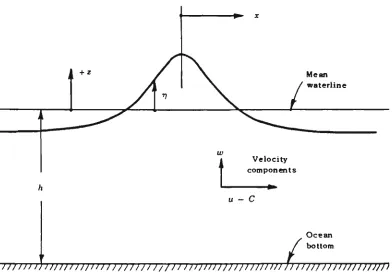
Figure 2.5. Schematic representation of a small amplitude wave.

The Cartesian coordinate system has its origin located on the still water

level (SWL) and the depth, h, of the water is measured from the sea bed to

the SWL. The wave is of height, H, has a wavelength, L, and a phase

velocity or celerity, C. rj denotes the elevation of the free surface

from the SWL at any position x and time t.

velocity normal to sea bed must be zero. The bottom boundary condition may

therefore be written as

w

-il^ 0

If it is assumed that the pressure on the free surface is zero (gauge) at

any position x or time t and that the flow is irrotational, the free

surface boundary condition is obtained by applying Bernoulli's equation at

the free surface (z " n)• Furthermore, by neglecting the second order

terms to satisfy the small amplitude assumptions, the linearized dynamic

boundary condition is

1 £§

g St at z

7 = 0 (2.35)

In physical terms the linearization assumes that the flow is sufficiently

small to render the kinetic energy of the fluid particles negligible

compared with the total mechanical energy in the system.

Since no particle can cross the free surface, the particle velocity at the

free surface must be equal to the normal velocity at the free surface. If it is assumed that the water surface elevations are small relative to the

wavelength, the rate of change of elevation of the water surface at any point may be said to be approximately equal to the vertical velocity

component, w, at the same point

w ^±1

dt

therefore

Sn 4. ST]

St

0

(2.36)

In

at z = 0 (2.37)

Since

The linearized free-surface boundary conditions of equations (2.35) and (2.37) may be combined by eliminating rj to obtain

i . A _ i + i i - 0 for z " -n ^ 0 (2.39) S st^ ^^

Since a continuous fluid within the wave is being considered and

irrotational flow is assumed, the differential equation to be satisfied within the region -h < z < +TJ and -« < x < +« is the

two-dimensional form of Laplace's equation which is written as

sh ^

5 ^ ^ Q (2.40)

5x^ Sz^

Using the method of seperation of variables, in which the solution of the partial differential equation is assumed in product form, the general solution of equation (2.40) may be written as

§Cx,z,t; = X(x) Z(z) T(t) (2.41)

where X is a function of x alone, Z is a function of z alone, and T is a function of t alone.

Substituting equation (2.41) into equation (2.40), dividing by X(x)Z(z)T(t) then seperating the variables yields

!

_ dfx _ _ J_ df2__ _

^ (2.42)

X dx^ Z dz^

where the constant k is the wave number. The general solutions for X(x) and Z(z) respectively are

X(x) =• (72 sin(kx + ^) (2.43)

and

vhere C^ , Cn , a and 3 are arbitrary constants. The

particular solution of Z(z) is obtained by applying the boundary condition

at the sea bed so that equation (2.43) is satisfied at z =• -h. Hence

^ ' Cr, k sinh(-kh + a) ' 0 dz ^

(2.44)

from which a - kh. Equation (2.43) therefore becomes

Z(z) = C2 cosh(kz + kh) (2.45)

By substituting equations (2.41) and (2.45) into the linearized

free-surface boundary condition (eqn. 2.39) the solution of the time

function, T(t), is

A cosh(kz + kh) ^ ^ + sinh(kz + kh)

I g dt^

- 0 _(2.46)

z=0

When the seperation of variables is applied, equation (2.46) becomes

Ail^J- -0

T dt^

where co is the wave circular frequency and is expressed as

(2.47)

CO = [kg tanh(kh)] 0.5 (2.48)

The general solution of equation (2.47) is

T(t) - C-, sin(uit + 1) (2.49)

By equating the phase angles /3 and 7 to zero and combining

equations (2.43), (2.45) and (2.49), the solution to the differential

equation according to equation (2.41) can now be expressed as

i(x,z,t) - A cosh(kz + kh) sin(kx) sin(oot) (2.50)

where the arbitrary constants C-, , C2 and Co are now represented by

Substituting for the velocity potential in the dynamic free-surface

condition yields the expression for the displacement of the free surface of a standing wave:

r7--iii

g 5t _{Z'O S} - - — cosh(kh)- sin(kx)- cos ((jit)

- a sin(kx)' cos((^t) (2.51)

where a is the wave amplitude. By replacing the amplitude coefficient A in equation (2.50) by -ag/ui cosh(kh) , one obtains

i(x,z.t) - - f _ g cosh(kz + ich;.^_.^^^^ ^^^^^^ ^2.52) 00 cosh (kh)

From the combinations of the sine and cosine functions of x and t, there exist three additional standing wave solutions. The four standing waves are

rij^ = a sin(kx)- cos(ut) (2.53)

T]2 ^ a. cos (kx) • cos ("cot; (2.54)

ri2 = a sin(kx)- sin(ut) (2.55)

r ? ^ = a cos(kx)- sin(u>t) (2.56)

Since the above expressions result from the solution of a linear equation, any pair can be superimposed to obtain solutions describing travelling waves:

T]~='rij^ + T]^ = a sin(kx + cot) (2.57)

for left-running waves, and

ri^ = ri2 + n2''^ ^°^(^ - ^^) (2.58)

for right-running waves. The velocity potential functions corresponding to equations (2.57) and (2.58) are respectively

^- . _ a g cosh(kz + kh) _,^,^j,^ + ^t; (2.59)

and

i^ . a j COsh(kz -H kh) , ^ . „ ^ ^ ^ ^^^ ^ ^ ^ 0 ^

to cosh(kh)

If the origin of the coordinate system is allowed to travel with the wave, then the argument of the cosine term in equation (2.58) is constant, or

kx - cot - constant (2.61)

and the differential of the argument is

k dx - (uo dt = 0 (2.62)

The wave velocity or celerity is therefore defined as

C ^ ^ - ^ ^ k ^ f L (2.63) dt k T

where f is the wave frequency, L the wavelength, and T the wave period. The combination of equations (2.48) and (2.63) yields an expression for the wave celerity

C = 1. tanh(kh) <2-^^^ k

and a transcendental equation for the wavelength

^ T2

L = C T = M-L tanh(2nh/L) (2.65) 2n

For deep water waves, customarily defined when the water depth is greater than twice the wavelength, or h/L > 2 , Kinsman (1965), equation (2.65) reduces to

L = gr^/2n (2.66)

equation (2.65) is written as

L = gT^ h/L (2.67)

In considering the fluid particle motion, equations (2.12) and (2.60) are combined to give the velocity components of the fluid in a right-running wave as

5§ a__g_k cosh(kz + kh) ^^^^^ _ ^^^ ^2.68)

Sx CO cosh (kh) and

v - 5 $ ^ S k sinh(kz + kh) ^^^^^ _ ^^^ (2.69)

Sz CO cosh(kh)

It is evident from equations (2.68) and (2.69) that the fluid particle velocities u and w vary sinusoidally in time with a mean position at a fixed point (XQ,ZQ). The fluid particle displacement equations are

obtained by integration of the particle velocity equations with respect to time yielding

i = - ^ g ^ cosh(kzQ + kh) s^n(kxQ - cot; (2.70) CO cosh (kh)

for horizontal particle displacements and

^ = ^ S k sinh(kzQ + kh) cos(kxQ - cot) (2.71) 2

CO cosh (kh)

for vertical particle displacements.

It can be seen from equations (2.70) and (2.71) that the paths of the fluid particles about a mean position (XQ,ZQ) are determined by the ratio of

the water depth to the wavelength, h/L = kh/2n. For deep water waves (0.5 < h/L) the fluid particles move in a circular path which radius decreases exponentially with depth. The fluid particles motion of

major and minor axes decreasing exponentially with depth. For waves in

shallow water (0 < h/L < 1/20), the fluid particles motion is approximated by an eliptic path with the major axis independent of depth as illustrated

in figure 2.6.

miin/m/mwi/iiimiiiii/

Shallow water

L 20

Intemiediate depth

J- < iL < i

20 L 2

wnmmmmnmrmm

Deep water

A > i

L 2

Figure 2.6. Effects of water depth on fluid particle paths.

2.4. Finite Amplitude Waves.

The small amplitude wave theory, presented above, is founded on the premise that the fluid motions are sufficiently small to permit the linearization

of the free surface boundary conditions. Alternatively the validity of the small amplitude wave theory may be defined by

JL

« 1

« 1

or by the Ursell parameter

U„ -MA. < 15 h^

(2.73)

Since these assumptions are no longer valid if the wave amplitudes are finite, it is necessary to retain the higher-order terms to achieve an

accurate representation of the nonlinear wave motion to allow for cases where H/h and H/L approach 1. In order to eliminate the difficulties in

H/L « 1). The validity of various classical wave theories according to

ranges of these important parameters are shown graphically in figure 2.7.

0.001

Figure 2.7. Classification of wave theories.

After Le Mehaute (1976)

-The formulation of the finite amplitude wave boundary value problem is

basically the same as that presented for the small amplitude wave theory

with the exception that the nonlinear higher order terms are retained. For convenience, it is generally assumed that a wave travels at a constant

celerity c and with retention of its shape. A right-running wave of finite

amplitude within a rectangular coordinate system, whose origin travels with

the wave crest at a velocity c, as shown in figure 2.8, is considered.

Since, as in the analysis of linear small amplitude waves, the fluid is

assumed to be incompressible and irrotational, Laplace's equation is

applied

5^$ 5^$

5x2 Sy2

S^

sz'

u - C

)nfn)))}}}))) ))nn)))nnn//nn)))ntnn)i))in) II i}n}nn)i}}}7}}}}

L

Ocean bottom

Figure 2.8. A stationary finite amplitude wave.

The boundary condition at the bottom is such that there is no flow across the boundary and is written as

w 5$ _5z 0 at z = - h (2.75)

There are two boundary conditions at the (stationary) free surface that must be satisfied. The dynamic boundary condition is the requirement that

the total energy along the free surface remains constant. This is

expressed as Bernoulli's equation applied to the quasi-steady flow at the surface

7 9 9

??+-=- (u - C) + w^ = Q at z = n 2g

(2.76)

The kinematic free surface boundary condition requires that no fluid be

transported across the free surface. This can be formulated by specifing that the resultant vector of the fluid velocity at the free surface be

tangent to the free surface.

5x (u - C) at z (2.77)

Equation (2.77) may be expanded by the Maclaurin series in which

,, -^ , , = Z i c " - I + k + k 2 + ^ +

(^ - ^> n=0 (2.78)

Since

Srj ^ w

Sx (u - C) w C (1 - u/C)

(2.79)

then equation (2.77) becomes

ST] _ 5^ _ 2^ f^ 5^ n-o' ^

n

w wu wu WW

if f l + H + [ii

C L C \C

+ (ii _(2.80)

In summary, the derivation of an accurate finite amplitude wave theory was

achieved by finding a solution to Laplace's equation which satisfies the boundary conditions as expressed in equations (2.75), (2.76) and (2.77).

2.5. Stokes Wave Theory.

The nonlinear Stokes wave theory was developed by assuming that the

solutions to the properties of wave motion, such as the velocity potential,

the free surface displacement and the wave celerity can be represented by a

$ - Z e" §^ (2.81) n~l

n - I. e'^ n^ (2.82) n-l

and

$ - C^ + 2 e" C^ (2.83)

n-1

Where C.^ is the lowest order celerity term and is equivalent to equation (2.64). In the solutions above, the sum of the terms up to index n

represent the n order theory. Accordingly, as the number of terms increases, so does the accuracy of approximation to the actual wave properties. The solutions to equations (2.81), (2.82) and (2.83) are obtained by successive approximations and require numerous and detailed

calculations of the coefficients and parameters in which small errors often occur. Consequently, there often exist differences in the final results of

various investigators. As the development of Stokes theory is rather involved, the reader is refered to Kinsman (1965) for a thorough review of Stokes pertubation method.

The results of Stokes first order analysis are identical to those of the

linear, small amplitude wave theory.

When extended to the second order, the solutions to the finite amplitude

Stokes analysis are, for the velocity potential:

^ ^H c co^rfc/^ + kz) _ ^j_^(f^ _ ^^) ^

2 sinh(kh)

Ai 3nC_ cosh(2kh 4- 2kz) , ^-^ ^2kK - 2u>t) (2 .84) 4 41 sinh^(kh)

n - l cos(kx - oot) ^iJASSflll^

2 4 2L sinh^(kh)

[2 + cosh(2kh)] cos(2kx - loot) (2.85)

and for the wave celerity:

£.tanh(kh) - C^

k (2.86)

The wavelength is given by

L - ^.tanh(2Kh/L)

2n (2.87)

The first term of the free surface profile (eqn. 2.85) is the same as the

solution to free surface profile of the linear small amplitude theory while the remaining term is the second order correction for nonlinearity.

However, the expressions for the celerity and the wavelength are identical to those described for the first order small amplitude theory.

Unlike the linear theory, Stokes' second order theory describes a wave form that is asymmetrical about the mean water level as shown in Figure 2.9.

Still-water level Mean water level

Figure 2.9. Second order Stokes wave.

Solutions for the third and higher order Stokes waves that take into

account more terms to improve the approximation have been derived and are given in the Shore Protection Manual (1984).

2.6. Cnoidal Wave Theory.

Long waves of finite amplitude in shallow water are presently best

described by the cnoidal wave theory. It is based on the assumption that

the square of the slope of the water surface is small relative to unity.

The cnoidal wave is periodic and has sharp crests separated by wide troughs

as shown in Figure 2.10. The surface profile of the cnoidal wave is given by the Jacobian elliptical cosine function, hence the term cnoidal.

Solutions for the cnoidal water surface profile, wave celerity and

wavelength may be found in the Shore Protection Manual (1984).

The cnoidal wave theory is considered only valid for h/L < 1/8 and Up > 26. As the wave height becomes small relative to the water depth,

the wave profile approaches a sinusoidal profile as predicted in the

linear small amplitude theory. However, when the wavelength increases and

approaches infinity, the cnoidal wave theory reduces to the solitary wave theory.

2.7. Solitary Wave Theory.

The solitary wave theory describes a wave of permanent form and of infinite wavelength. A solitary wave is neither oscillatory nor does it have a

trough as it lies entirely above the still water level. The profile of a solitary wave is illustrated in figure 2.10. Equations defining the

solitary wave profile and the wave celerity are outlined in the Shore Protection Manual (1984).

2.8. Stream Function Wave Theory.

A numerical approximation to solutions of the hydrodynamic equations

describing wave motion have been proposed by Dean (1965). The stream

function wave theory (more accurately described as a procedure), is a

nonlinear theory based on a stream function representation of the flow.

The theory is similar to that of Stokes in that it is constructed in terms

of sine or cosine functions that satisfy the original differential

equation (Laplace's equation). However, the coefficient of each higher

AIRY WAVES

^7^^*^.'"'•'.*.'.*^'J'.'.''P'"'.'.>T*;*?»7^7^,''.'^.'.'•^'.'.'.'?''T^^'T*T*^'T*?*T*T'.'.'•'•'!''•'.*.''•*•'^

STOKES WAVES

r^p > F'p I"

CNOIDAL WAVES

SOLITARY WAVES

. . . J . 1 . 1 . 1

Figure 2.10. Illustration of various wave profiles.

2.9. Wave Superposition - Small Amplitude Waves.

Due to the linearity of Laplace's equation for small amplitude waves, the

total velocity potential of the wave field, ij., is equal to the sum of the velocity potential of each individual wave:

N

n-1

(2.88)

where N is the total number of individual waves and

$n - fn_! g o ^ ^ C y + ^n^> . cos(k^x + co^t + 5„;

co^ cosh(k^h)

in which S is an arbitrary phase relationship between various

individual waves.

By applying the linear boundary conditions for small amplitude waves, as in section 2.3, the resulting water surface displacement is given by

N

rjj ~ "^ Tin (2.90) n'-l

When a number of small amplitude waves travelling in the same direction in water of constant depth are considered, the water surface displacement may

be written as

N

^T ' ^ ^n s^n(knX " "n + ^n> (2.91) n-1

If the frequency of each individual wave is the same then

^ 2 = co^ = coj = . . . . co^ (2.92)

and

kl ' k2 - kj = . . . . k^ (2.93)

Using the trigonometric identity

sin(A + B; = (sin A • cos B) + (cos A • sin B) (2.94)

equation (2.91) may be written as

N N rjj, = sin(kx - cot) Z a cos(S^) + cos(kx - cot) S a sin(S ) (2.95)

n-1 n-1 If the summations in equation (2.95) are substituted such that

N

2

n-1

2 a^ cos 5^ = r cos A (2.96)

N

2 a^ sin 5_ = r sin A

n-1 (2.97)

then equation (2.95) becomes

•q^ - r sin(kx - cot) cos(X) + r cos(kx - cot) sin(X) (2.98)

or

rjj. - r sin(kx - cot + X) _(2.99)

where r and X are dependents of the amplitudes and phases of the

individual waves and are written as

r = ( 2 a^ cos 5„;2 + C 2 a^ sin S^)'

. n-1 n-1 (2.100)

and

A = tan

N

2 a„ sin 5„

n-1

N

2 a„ cos 5„

n-1

(2.101)

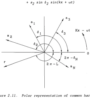
This resulting harmonic oscillation is best illustrated when presented in

polar coordinates as shown in figure 2.11.

When two harmonic progressive waves of the same frequency travelling in

opposite directions are combined, the resulting water surface displacement, obtained by addition of each individual wave, is written as

r]j, = ai sin(kix - ooit + Si) + ao sin(k2X + 002^ + 5^; _(2.102)

Again, by using the trigonometric identity of equation (2.94) equation

rij - a J sin(kx - cot; + ao cos 5^ s i n ("/ex + cot;

+ 32 sin S2 sin(kx + cot) (2.103)

Kx - cjl

Figure 2.11. Polar representation of common harmonics of arbitrary phase.

When the above wave system is considered such that the outgoing wave is generated by the perfect reflection of the oncoming wave from a vertical wall, the amplitude of the reflected (outgoing) wave will be the same as

that of the incident (oncoming) wave. Since the wave frequency co, and hence the wave number k, are assumed to remain constant, the reflection coefficient, K , defined as the ratio of the amplitude of the incident wave to the amplitude of the reflected wave, or

Kj. = 3^/32 (2.104)

must be equal to unity.

The velocity potential of the wave system is obtained by superposition of the velocity potential of each individual wave and is written as

The boundary condition at the impermeable plane vertical wall (x = B) is such that the horizontal partical velocity, Uj, is zero or

S§rr,

Urj, i = 0 at X - B for all t (2.106) ^ Sx

By differentiating equation (2.105) and applying the above boundary condition at x = B

sin(kB - cot; = sin(kB + 5^; (2.107)

Applying the trigonometric identity of equation (2.94),

sin(kB) cos (cot) - cos(kB) sin(oot) = sin(kB + 62) cos (cot)

+ cos(kB + 5^; sin(cot) (2.108)

and equating the sinusoidal and cosinusoidal components,

sin(kB) = sin (kB + 62) (2.109)

and

cos(kB) cos(kB + S2) (2.110)

Ic follows that

62 - n(2n + 1) - 2kB for n =- 0, 1, 2, . . . (2.111)

By substituting for S2 in equation (2.103), and expanding

rjrp = a sin(2kB) cos(kx) cos (cot) - a sin(2kB) sin(kx) sin(cot) - a cos(kx) sin(cot) - a cos(2kB) sin(kx) cos (tot)

+ a sin(kx) cos (cot) - a cos(2kB) cos(kx) sin(cot) (2.112)

By introducing the following trigonometric identities:

and

cos(2kB) - 2 cos'(kB) - 1 = 1 - 2 sin'(kB) (2.114)

equation (2.112) reduces to

rjj, - 2a sin(kB - cot) cos(kx - kB) (2.115)

which is the equation for a standing wave or clapotis, the nodes of which are located at

cos(kx - kB) = 0 (2.116)

or

""node - B -''(''' + ^>. for n - 0, 1, 2 , . . . (2.117) 2k

and the antinodes at

cos(kx - kB) = + 1 (2.118)

or

""antinode = ^ " ""A for n - 0, 1, 2 , . . . . (2.119)

If the boundary, B, is made to be at x — 0, the phase of the reflected wave is reduced to S2 =• n(2n + 1) . Consequently, for n = 0, equation

(2.115) reduces to

rij. 2a sin (cot) cos(kx) (2.120)

When energy dissipation and/or transmission occurs, the reflection is not perfect and the reflection coefficient, K , will therefore be less than unity.

waves, is written as

T}j - aj^ sin(kx - oot) + a2 sin(kx + cot + S2) (2.121)

If it is assumed that the incident wave is partially reflected from a

vertical wall located at x — 0 and that the phase of the reflected wave is n as for the perfect reflection case, then equation (2.121) reduces to

rjj, = a^ sin(kx - oot) - K^a-j^ sin(kx + cot; (2.122)

where K ai = ao

The addition and subtraction of the term K^a-isin(kx - cot; yields

rjj = aj^(l-K^)sin(kx - cot) - 2K^a-j^ sin(o3t) cos(kx) (2.123)

in which a progressive wave and a standing wave are represented by the first and second terms respectively. It can be seen that, as the

reflection coefficient increases, the amplitude of the progressive wave component decreases, and, in the limit when K = 1, equation (2.123) reduces to equation (2.120). Alternatively, equation (2.123) may be written as

Hj - aj^(l-K^)sin(kx) cos (cot) - a-j^(l+K^) cos(kx) sin(cot) (2.124)

The time at which extremes of rjj. at any location, x, occur may be

obtained by differentiating equation (2.124) with respect to time, thus

Sr]j,

= 0 (2.125) X

St

resulting in

[cot]„ = tan' 'Tmax

- ^I^^ "^ ^r^ cot(kx) L 32(1 - icp

(2.126)

By substituting ^Tmax ^^^ ^T ^^^° equation (2.124), the

STI

Tmax - 0

5x

(2.127)

resulting in

[kx]. - nn and i (2n + 1) ^Tmax 2

(2.128)

where n - 0, 1, 2,

Substituting for oot and kx into equation (2.124), it can be seen that the resulting function describes a "standing" wave in that the amplitude envelope is stationary with extremes a and a^ at the nodes and

antinodes respectively, where

i^ - a^(l - K^) (2.129)

'h '^l(l ^

V

The reflection coefficient may therefore be obtained from the envelope of the wave amplitudes from

K, ^h - ^1 au + a.

(2.131)

or, for small amplitude waves where H = 2a,

"h^"x

(2.132)

where H L and H are defined in figure 2.12.

3. STATISTICAL ANALYSIS OF OCEAN WAVES

3.1. Spectral Analysis of Random Processes.

The study of ocean waves has developed as a combination of time series analysis and statistical geometry governed by the laws of hydrodynamics. In this chapter nondeterministic methods of describing the structure of the wave disturbed water surface are presented. The basic ideas of spectral analysis are first considered followed by a review of spectral models of ocean waves. The probability distributions of sea surface parameters, which give concise and useful properties of water waves, are also examined.

Random processes are generally classified into three categories: (1) nonstationary, (2) stationary and (3) stationary and ergodic. A random process is said to be stationary when the governing statistical

characteristics are time invariant. A stationary process is ergodic if any finite record if completely representative of the whole, infinite process. Since any record of ocean wave data is of finite duration, ergodicity has to be assumed. Furthermore, since it is never possible to demonstrate ergodicity, one is forced to make the ergodic assumption.

Although no two wave records are ever identical, they will possess certain identifiable statistical properties. Sverdrup and Munk (1947)

characterised a random sea by introducing the concept of the significant wave. Where the variety of wave forms is great, such as in a random sea, characterisation by a single wave form is inconsistent with the random nature of the process.

Longuet-Higgins (1957) described ocean waves by treating the random process as a combination of an infinite number of monochromatic waves of different amplitude, frequencies, directions and phases expressed as

00

where a is the wave amplitude, k is the wave number, 9 is the wave direction, f is the wave frequency and 5 is the phase angle.

Although the correctness of this interpretation of random ocean waves as a linear superposition of free progressive waves cannot be proven, it has been successfully used to characterise most properties of ocean waves. This interpretation of ocean waves rests on four conditions: (1) the

frequencies f^ must be densely distributed between zero and infinity such that an infinitesimal interval df contains an infinite number of

frequencies f^. (2) the wave directions 9 must be densely

distributed between -n and n such that an infinitesimal interval d9 contains an infinite number of directions 9 . (3) the phase

angle 5^ must be randomly and uniformly distributed between 0 and

2n. And (4) although the amplitude of each wave is infinitely small, 2

the summation of a^ should have a finite and unique value G(f,9) expressed as

f+df 9+d9

2 2 0.5 a^ = G(f,9) df d9 (3.2)

f 9

The directional wave spectrum G(f,9) defined by equation (3.2) is an

expression of the distribution of wave energy with respect to frequency and direction. When waves are observed at a fixed single point in the ocean, the wave profile is expressed as

n(t) = 2 a„ cos(2nf^ + S^) (3.3) n=l

The sum of the squares of the wave amplitudes over an interval f to f+df is given by

f+df

2 0.5 a^' = G(f) df (3.4) f

considered. Random waves will therefore be represented in the frequency domain by the frequency spectrum . The use of spectral or frequency analysis to describe ocean waves has now been well established and is discussed by Kinsman (1965).

Linear physical systems are defined as being additive and homogeneous. Specifically, a system is additive when the response to a sum of inputs equals the sum of the responses due to each individual input. If y(x) is the response to an input x^ then

y(xj^ + x^; = 7CX2; + y(x2) (3.5)

A system is considered homogeneous if the response to a an input,x , times a constant, c, is equal to the constant times the response of the input alone, or

y(cx) - c y(x) (3.6)

Consequently, when the random input into a linear system is Gaussian, the response will also be Gaussian.

The mathematical basis of spectral analysis is the Fourier Transform which assumes that the signal is composed of a number of sinusoidal or

cosinusoidal components of various frequency, amplitude and initial phase. The one-sided discrete Fourier Transform of a sampled time signal g(t) is given by

n-1

^(^k^ ' i ^ S(^J exp(-j2Tmk/N) (3.7)

where k and n are positive integers. It can be seen from equation (3.7) that in order to obtain N frequency components from N time samples requires

2

N complex multiplications. Since its introduction in the mid 1960's,

the alogarithm known as the Fast Fourier Transform or FFT which obtains the same results with Nlog2(N) complex multiplications has been widely used.

Power Spectral Density, or PSD, wich has the units of energy per unit

frequency or, in the case of water surface elevation, or/Hz.

The frequency response function of a. system represents the output to input

ratio in the frequency domain and as such characterises stable, linear,

stationary systems. The relationships between the input signal a(t) and the output b(t) of a stable, linear, stationary system in the absence of

noise are shown in figure 3.1.

a(t)

A(f) - *

hit)

Hlf)

b(t) = a{t) • h(t)

B(f) = A(f) • H(f)

Figure 3.1. Linear system input - output relationships

The system is characterised in the time domain by its impulse response h(t)

and the output signal b(t) is the convolution of aCt; with h(t) or

b(t) - a(t) * h(t) (3.8)

where * indicates convolved with. Application of the convolution theorem

yields

B(f) - A(f) H(f) (3.9)

where A(f) is the Fourier transform of a(t), B(f) that of b(t) and H(f)

that of h(t). A more thorough discussion of the convolution theorem is

presented by Randall (1987).

The frequency response function, H(f), of the linear system in the absence

of noise is obtained by

If noise is present in the output signal, errors in the result are

minimized by multiplying the numerator and denominator of equation (3.10) by the complex conjugate of the Fourier transform of the input thus.

H.(f) -^(f> A (f) = (^AB(^) (3-W

'AA''

A(f) A*(f) G.Jf)

which represents the one-sided cross spectrum normalised by the one-sided autospectrum of the input.

It has been shown by Bendat and Piersol (1971 & 1986) that the normalized standard error (random portion of estimation error) in spectral density

estimates of a stationary (ergodic) Gaussian random process, obtained by the Fourier Transform, is a function of the bandwidth, B^ (Hz), of the measurement and the record length T (sec) written as

^r

' VCBgr;^--^

(3.12)

For a raw spectral estimate, it turns out that

Bg = Af = 1/T (3.13)

It follows, from equation (3.12), that the normalized standard error of a raw spectral estimate is unity. This indicates that the standard deviation of the estimate is equal to the value of the estimate, hence poor accuracy is obtained.

The distribution of each frequency component of the estimate may be approximated by a chi-square distribution, ;

statistical degrees of freedom, n, being 2. 2

approximated by a chi-square distribution, x„ . with the number of

Furthermore, it can be seen from equations (3.12) and (3.13) that an

increase in record length will not yield improvement of the random error of spectral estimates.

raw spectral estimates from independent sample records is computed. This method requires the measurement and analysis of a number of independent

records. The second method of improving the accuracy of spectral estimates is by smooching of the estimate over frequency by averaging a number of

adjacent spectral components according to one of several weighting

functions. Smoothing by this method is usually performed on the estimate from a single sample record. This technique is only valid under the

assumption that the spectral density varies only gradually with respect to frequency.

If p adjacent frequency components of the raw spectral estimates are averaged, the smoothed spectral estimate will be a yc variable with approximately n - 2p degrees of freedom. The resulting effective resolution bandwidth becomes

Sg = p/T (3.14)

so that the normalized standard error is given by

Similarly for ensemble averaging

where N^ is the number of raw spectral estimates, and for a combination of both frequency smoothing and ensemble averaging, the normalized standard error is given by

e^^ l/(pN^)^-^ (3.17)

It can be seen from the above analysis that smoothing of raw spectral estimates by averaging adjacent estimates always results in loss of

3.2. Spectral Models of Ocean Waves.

There have been numerous attempts at formulating mathematical spectral models of ocean waves and there now exists a number of empirical and

semi-empirical frequency spectrum models. These mathematical models,

generally based on one or more parameters such as the significant wave

height, wave period, shape factor, wind velocity, etc., are usually derived

from experimental ocean wave records and hydrodynamic theories.

The Neumann spectral model was developed in 1953 and is expressed in terms of prevalent wind velocity, U^, and is written as

G(ui) - Boo-^ exp[-2g^/(dU^)'] (3.19)

In which B is a dimensional constant. As one of the earlier mathematical

models, it was derived from limited data. With later developments in measurement techniques, the shortcomings of this model have been

demonstrated and it is now regarded as outdated.

The majority of recent spectral models are based on the spectral function proposed by Phillips (1958) who defined the equilibrium range of the

frequency spectrum for a fully developed sea as

G(ui) - ag'(ijo)-^ (3.18)

where a is the Phillips constant, g the acceleration due to gravity and CO the angular wave frequency.

Although seldom employed in practice, the Phillips spectrum has been used

as a basis for the formulation of other spectral models.

The Bretshneider spectrum, developed in 1959, may be used to represent

fully-developed sea conditions. The model is based on the assumptions that

the spectrum is narrow-banded and that the distribution of the wave height and wave period follow the Rayleigh distribution. It is written as

where H^ is the significant wave height in feet, T the significant wave period in seconds defined as the average period of the significant waves and co_ - 2nT^. _{s s}

In 1964, a slight modification to the Bretshneider spectrum was suggested at the International Ship Structures Congress. The ISSC spectrum is written as

G(oi) - 0.1107(H^)'(^)^(co)'^ exp[-0.4427(co/oo)^] (3.23)

where ZS — 1.296 OOQ in which OOQ is the spectral peak frequency.

Pierson and Moskowitz (1964) developed a spectral model also based on wind velocity. This model, commonly referred to as the P-M spectrum, is based on more accurately recorded data and represents a fully developed sea state. It is formulated on the assumptions that the wind has blown at a steady velocity and fixed direction for many hours over a large area.

Despite the fact that the model is derived from steady sea and wind conditions and that ocean waves rarely approach a fully developed sea state, it has been widely used in the design of offshore structures to represent severe storms. The P-M spectrum is

G(co) - ag'uT^ exp[-0.74(uo U^/g)-^] (3.20)

Where a - 0.0081

and U - prevalent wind velocity [ft/s] at 54 ft above the mean sea level.

Alternatively, the P-M spectrum may be expressed in terms of spectral peak frequency, COQ, as

G(co) = ag^co"-^ exp[-1.25(co/ooQ)-^] (3.21)

The International Towing Tank Conference (ITTC) spectrum is a modified

The P-M, Bretshneider, ISSC and ITTC spectral models are of the same class

and may all be described by a two parameter spectrum expressed in terms of

a statistical wave height and a characteristic wave period as shown by

Chakrabarti (1987). Since the P-M based and Bretshneider based spectral

models rely on wind speed measurements taken at different heights above the

water surface, the difference between the two forms may be considerably

reduced by taking into account the gradients of the wind velocity with

respect to altitude.

The Scott spectral model, developed in 1965, is independent of wind speed,

fetch or duration and was formulated to represent the spectrum of a

fully-developed sea. It is expressed in terms of significant wave height

and spectral peak frequency as.

G(co) = 0.214 HJ exp

(00 - . , ) ' \0-'

\0.065(co - COQ + 0.26)J

for - 0.26 < (co - co^; < 1.65 (3.25)

G(co) — 0 elsewhere

where H is the significant wave height in feet.

Derived from wave data recorded on Lake Michigan, the Liu spectral model

was developed in 1971 and contains a fetch-dependence parameter. The model

is similar in form to the P-M spectrum and is written as,

G(co; = ag'(XQ)-^-'^(i^)-^ exp[-0(oo U^/g)-^X(j-^/^] (3.26)

where a = 0.4, 13 = 5500, Xg = gX/uJ- and U^ = U^(U^/gX)^^^ in which U^

is the wind velocity at 10 metres.

Mitsuyasu (1972) proposed another fetch-limited spectral model based on

data recorded from waves generated in a laboratory and in a bay. Unlike an

earlier model, which did not give consistent results at low frequencies,

this revised model of the fetch limited spectrum consists of two parts and

is written as,

where a - 9.12 x 10~^^ and 3 = 3.55, and

, G(co; - ag'(ao)-^(XQ)-^-308 co > co^ (3.28)

where a = 0.589.

Since both the Liu and Mitsuyasu spectra are fetch dependent and are based on lakes and reservoirs of limited fetch, they may have limited application in ocean conditions.

The JONSWAP spectrum was developed during the Joint North Sea Wave Project by Hasselman et. al. (1973). The model was derived from experimental data based on unsaturated (or not fully developed) sea conditions. Comparison between the experimental JONSWAP spectrum and the P-M spectrum showed discrepancies near the spectral peak. The JONSWAP model is therefore basically the P-M model with an additional peak enhancement function and is expressed in terms of five parameters. Even though three of the five

parameters may be reduced to constants via empirical relationships, the model is somewhat inaccurate and inconvenient to use since the agreement between some of these empirical formulae and the data are rather crude as shown by Hasselman et. al. (1976). The JONSWAP spectrum is written as

GCco; = ag^co-^ expl-1.25(co/u>Q)-''] jexp[-(oo-Oo)'/(2r'c,o')] (^.24)

Where 7 is the peakedness parameter and r the shape parameter. For a prevailing wind of velocity U (in ft/s at 54 ft above the mean sea level) and a fetch X (ft), the parameters are defined as

1 < 1 < 7 ( average = 3 .3 ) .

T = 0.07 for CO < U)Q (considered fixed). T = 0.09 for CO > COQ (considered fixed) .

a = 0.076 (XQ)~^-'' (a = 0.0081 when X is unknown). CO - 2vi (g/U^) (XQ)~^'^^ (frequency in rad/s)

^0

=

sx/uj