Simple composition theorems of one-way functions -- proofs and presentations

(1)

Simple composition theorems of one-way functions

– proofs and presentations

Jaime Gaspar

∗

Eerke Boiten

†

December 18, 2014

Abstract

One-way functions are both central to cryptographic theory and a clear example of its complexity as a theory. From the aim to understand theories, proofs, and communicability of proofs in the area better, we study some small theorems on one-way functions, namely: composition theorems of one-way functions of the form “if f (or h) is well-behaved in some sense and g is a one-way function, then f◦g (respectively,g◦h) is a one-way function”.

We present two basic composition theorems, and generalisations of them which may well be folklore. Then we experiment with different proof presen-tations, including using the Coq theorem prover, using one of the theorems as a case study.

1 Composition theorems

1.1 Introduction

One-way functions are perhaps the most basic building blocks in cryptography. The basic building blocks are composed in order to produce more complicated structures. So composition theorems about one-way functions, that assert the behaviour of these basic building blocks under composition, seem fundamental to assess more compli-cated structures in cryptography. In this article we study two basic composition theorems, two generalisations of them, and then we use one of the generalisations as a case study in proof presentation.

Notation 1. Let us denote by P the set of all functions from{0,1}∗ _to_{₀_,₁_}∗ _that

are computable by a deterministic polynomial-time algorithm.

∗_{School of Computing, University of Kent, Canterbury, Kent, CT2 7NF, United Kingdom.}

Cen-tro de Matem´atica e Aplica¸c˜oes (CMA), FCT, UNL. [email protected] / [email protected], www.jaimegaspar.com / www.cs.kent.ac.uk/people/rpg/jg478. Financially supported by a Re-search Postgraduate Scholarship from the Engineering and Physical Sciences ReRe-search Council / School of Computing, University of Kent.

†_{School of Computing & Centre for Cyber Security, University of Kent, Canterbury, Kent,}

(2)

Informally, a one-way functiongis a function that is easy to compute but difficult to invert: x 7→g(x) is easy to compute but x←_[ g(x) (or more precisely, y ←_[ g(x) such thatg(x) = g(y)) is difficult to compute.

Definition 2 ([1, definition 2.2.1]). A functiong ∈ P is one-way if and only if

∀A, p,∃N: ∀n > N , Prg A(g(Un),1n)

=g(Un)

<1/p(n),

where

• A ranges over all probabilistic polynomial-time algorithms;

• p ranges over all positive polynomials with real coefficients;

• N and n range overN;

• the internal coin tosses of A are uniformly distributed;

• Un is a random variable uniformly distributed on{0,1}n;

• Pr is taken over Un and the internal coin tosses of A.

1.2 Specialised composition theorems

Theorem 3(left composition, particular variant). If f ∈ P is an injective function and g ∈ P is a one-way function, then f◦g ∈ P is a one-way function.

Proof (sketch). We essentially need to show that if Pr

g A(g(Un),1n)

=g(Un)

<

1/p(n), then Pr(f ◦g) A0((f ◦g)(Un),1n)

= (f ◦g)(Un)

< 1/p(n), and this is true taking A(x, y) =A0(f(x), y) and usingx=y ⇔ f(x) = f(y).

Definition 4 ([1, definition 2.2.4]). A function h ∈ P is length-preserving if and only if∀x∈ {0,1}∗_,_|_h₍_x₎_|₌_|_x_|_.

Theorem 5(right composition, particular variant). If g ∈ P is a one-way function and h ∈ P is a length-preserving injective function, then g ◦h ∈ P is a one-way function.

Proof (sketch). We essentially need to show that if Prg A(g(Un),1n)

=g(Un)

<

1/p(n), then Pr(g ◦h) A0((g ◦h)(U_n0),1n₎

= (g ◦h)(U_n0) < 1/p(n), and this is true taking A(x, y) = h(A0(x, y)) and making the change of variable Un = h(Un0),

which preserves probabilities because h|{0,1}n: {0,1}n → {0,1}n is injective and so bijective.

(3)

1.3 General composition theorems

A collision of a function f is a pair (x, y) such that x 6= y and f(x) = f(y). Informally, a collision-resistant function is a function such that it is difficult to find collisions. If we naively try to formalise this notion by

∀A, p, ∃N: ∀n > N ,

Pr[A(0,1n)6=A(1,1n)∧f(A(0,1n)) =f(A(1,1n))]<1/p(n), (1)

then: f is collision-resistant if and onlyf is injective. Informally this is because the existential choice of algorithm A allows the collision to be picked directly. Let us sketch a proof:

if f is not injective, then there is a collision (x, y), so the constant (on

z) algorithm A(0, z) = x and A(1, z) = y falsifies (1); if f is injective, then there is no collision, so the probability Pr[. . .] in (1) is 0, thus we have (1).

So the formalisation (1) is uninteresting as it reduces to injectivity. The problem, as suggested by the proof, is that if there is a collision (x, y), then the constant algorithm A(0, z) = x and A(1, z) = y satisfies the condition inside the brackets in (1). So we need to change (1) so as to exclude the constant algorithm.

• The traditional way of changing (1) is to replace a single functionf by a family

{fi}i of functions, randomly pick anfi and require that the algorithm outputs

a collision for this fi; since fi may change, the algorithm cannot be constant.

But this way forces us not to speak of “a collision-resistant function f” but rather of “a collision-resistant family of functions {fi}i”, which displeases us

[2, page 137] [3, lecture 21] [4, section 2.2].

• We propose another way of changing (1) by demanding that the algorithm outputs arbitrary large collisions, or equivalently, infinitely many collision; then the algorithm cannot be constant. This way allows us to continue to speak of “a collision-resistant function f” instead of “a collision-resistant family of functions {fi}i”, which pleases us.

We welcome comments on our proposed way of changing (1) resulting in the next definition.

Definition 7. A function f ∈ P is collision-resistant if and only if

∀A, p,∃N: ∀n > N , Pr[(|A(0,1n)| ≥n∨ |A(1,1n)| ≥n)∧

A(0,1n)6=A(1,1n)∧f(A(0,1n)) =f(A(1,1n))]<1/p(n),

where

• A ranges over all probabilistic polynomial-time algorithms;

(4)

• the internal coin tosses of A are uniformly distributed;

• Pr is taken over the internal coin tosses of A.

Definition 8. A function g ∈ P is length-nondecreasing if and only if ∀x ∈ {0,1}∗_, _|_h₍_x₎_{| ≥ |}_x_|_.

The following theorem almost generalises theorem 3 because collision-resistance generalises injectivity, but fails to truly generalise because it has the additional hy-pothesis thatg is length-nondecreasing. We welcome suggestions on how to dismiss this additional hypothesis.

Theorem 9 (left composition, general variant). If f ∈ P is a collision-resistant function andg ∈ P is a length-nondecreasing one-way function, then f◦g ∈ P is a one-way function.

Proof (sketch). We essentially need to show that if (a)g A(g(Un),1n)

=g(Un) has

low probability, then (b) (f◦g) A0((f◦g)(Un),1n)

= (f◦g)(Un) has low probability,

and this is true because

• (b) is the disjunction of

g A0((f ◦g)(Un)),1n

=g(Un) (c)

∨

g A0((f ◦g)(Un),1n)

6

=g(Un)∧

(f◦g) A0((f ◦g)(Un),1n)

= (f ◦g)(Un);

(d)

• (c) has low probability because it is (a) with A(x, y) = A0(f(x), y), and (d) has low probability because it is a collision of f (with |g(Un)| ≥n).

An unusual way of defining injectiveness (one-to-oneness) of a function h is to say ∀x∈ {0,1}∗_, _|_h−1_[_x_]_{| ≤}_{1. In the next definition, we generalise this by allowing}

q(|x|) (where q is polynomial) in place of 1.

Definition 10. A function h ∈ P is polynomial-to-one if and only if ∃q: ∀x ∈ {0,1}∗_, _|_f−1_[_x_]_{| ≤} _q₍_|_x_|_{), where} _q _{ranges over all positive polynomial with real}

coefficients.

The following theorem generalises theorem 5 because polynomial-to-oneness gen-eralises injectivity.

Theorem 11 (right composition, general variant). If g ∈ P is a one-way function and h ∈ P is a length-preserving polynomial-to-one function, then g ◦h ∈ P is a one-way function.

Proof (sketch). We essentially need to show that if Pr[g(A(g(Un),1n)) = g(Un)] <

1/p(n), then Pr

(g ◦h) A0((g ◦h)(U_n0),1n₎

= (g ◦h)(U_n0)

(5)

true taking A(x, y) = h(A0(x, y)) and p = p0q, and making the change of variable

Un =h(Un0), which increases probabilities at most q(n) times because

{x∈ {0,1}n_:_P₍_h₍_x₎₎_}₌[

y∈{0,1}n_:_P₍_y₎

h−1[y] ⇒

Pr[P(h(x))] = X

y∈{0,1}n_:_P₍_y₎

Pr[h−1[y]] = X

y∈{0,1}n_:_P₍_y₎

|h−1[y]|/2n ≤

X

y∈{0,1}n_:_P₍_y₎

q(n)/2n =q(n)X

y∈{0,1}n_:_P₍_y₎

1/2n=q(n) Pr[P(y)].

whereP is a predicate on {0,1}n _and _x _and _y _{are uniformly distributed on} _{₀_,₁_}n_.

Corollary 12(left and right compositions, general variant). Iff ∈ P is a collision-resistant function, g ∈ P is a length-nondecreasing one-way function and h ∈ P is a length-preserving polynomial-to-one function, then f ◦ g ◦ h ∈ P is a one-way function.

2 A case study in proof presentation

2.1 Introduction

Proofs in cryptography tend to be difficult to check due to the simultaneous use of four theories:

• probability theory (for example, when talking about the probability of certain events being low);

• computability theory (for example, when talking about certain problems being solved by probabilistic polynomial-time algorithms);

• asymptotic theory (for example, when talking about certain functions being negligible);

• cryptographic theory itself.

So proof presentation becomes especially important to facilitate to check proofs. In this section we show some possible proof presentations taking as a case study the proof of theorem 9.

2.2 Traditional proof

(6)

1. We assume

∀A, p, ∃N: ∀n > N , Pr[(|A(0,1n)| ≥n∨ |A(1,1n)| ≥n)∧

A(0,1n)6=A(1,1n)∧f(A(0,1n)) =f(A(1,1n))]<1/p(n), (2)

∀A0, p0, ∃N0: ∀n > N0, Prg A0(g(Un),1n)

=g(Un)

<1/p0(n), (3)

and we prove

∀A00, p00, ∃N00: ∀n > N00,

Pr(f ◦g) A00((f ◦g)(Un),1n)

= (f ◦g)(Un)

<1/p00(n). (4)

2. Let us take arbitraryA00 and p00. Taking

• A(i, x) to be the algorithm that uniformly and randomly choosesUn ∈ {0,1}n

and outputs

g A00((f ◦g)(Un), x)

if i= 0

g(Un) if i6= 0

in (2);

• p= 2p00 in (2);

• A0(x, y) =A00(f(x), y) in (3);

• p0 = 2p00 in (3);

we get N and N0 such that for alln > N00 = max(N, N0) we have

Pr[(|

=g(A00((f◦g)(Un),1n))

z }| {

A(0,1n)| ≥n∨ |

=g(Un)

z }| {

A(1,1n)| ≥n

| {z }

true

)∧

A(0,1n)

| {z } =g(A00₍₍_f_◦_g₎₍_U

n),1n))

6

=A(1,1n)

| {z } =g(Un)

∧f(A(0,1n)

| {z } =g(A00₍₍_f_◦_g₎₍_U

n),1n)

) =f(A(1,1n)

| {z } =g(Un)

)]<1/ p(n)

|{z} 2p00₍_n₎

,

Prg A0(g(Un),1n)

| {z }

=g(A00₍₍_f_◦_g₎₍_U n),1n))

=g(Un)

<1/ p0(n)

| {z } 2p00(n)

.

3. The condition (f ◦g) A00((f ◦g)(Un),1n)

= (f ◦g)(Un) in (4) is equivalent to

the disjunction

g A00((f◦g)(Un),1n)

=g(Un)

∨

g A00((f◦g)(Un),1n)

6

=g(Un)∧(f◦g) A00((f◦g)(Un),1n)

= (f◦g)(Un)

so

Pr

(f ◦g) A00((f ◦g)(Un),1n)

= (f ◦g)(Un)

≤

Prg A00((f ◦g)(Un),1n)

=g(Un)

+

Prg A00((f◦g)(Un),1n)

6

=g(Un)∧

(f◦g) A00((f◦g)(Un),1n)

= (f◦g)(Un)

<

1/(2p00(n)) + 1/(2p00(n)) = 1/p00(n).

(7)

2.3 Schematic proof

Proof. We essentially need to show that (f ◦g) A0((f ◦g)(Un),1n)

= (f ◦g)(Un)

has low probability, and we do this by showing that it is the disjunction of two conditions, each one with low probability:

(f◦g) A0((f ◦g)(Un),1n)

= (f ◦g)(Un)

⇔



           

           

low probability becausegis one-way

g A0((f◦g)(Un),1n)

=g(Un)

∨

g A0((f◦g)(U_n),1n)

≥n∨

true becausegis length-nondecreasing

|g(Un)| ≥n

∧

g A0((f◦g)(Un),1n)

6

=g(Un)∧

(f◦g) A0((f ◦g)(Un),1n)

= (f ◦g)(Un)

(8)

2.4 Calculus proof

fis collision-resistant

z }| {

∀p, A,∃N: ∀n > N , Pr[(|A(0,1n)| ≥n∨ |A(1,1n)≥n|)∧

A(0,1n)6=A(1,1n)∧f(A(0,1n)) = f(A(1,1n))]<1/p(n)∧

∀p, A0, ∃N0: ∀n > N0, Prg A0(g(Un),1n)

=g(Un)

<1/p(n)

| {z }

gis one-way

w

takeA(i, x) =

(

g(A((f◦g)(Un),1n)) ifi= 0

g(Un) ifi6= 0

,

p= 2pandA0(x, y) =A(f(x), y), and notice|g(Un)| ≥n

∀p, A, ∃N:∀n > N , Prg A((f ◦g)(Un),1n)

6

=g(Un)∧

(f◦g) A((f ◦g)(Un),1n)

= (f ◦g)(Un)

<1/(2p(n))∧

∀p, A, ∃N0: ∀n > N0, Prg A((f ◦g)(Un),1n)

=g(Un)

<1/(2p(n))

w

takeN= max(N, N0)

∀p, A, ∃N:∀n > N , Prg A((f◦g)(Un),1n)

6

=g(Un)∧

(f ◦g) A((f ◦g)(Un),1n)

= (f ◦g)(Un)

<1/(2p(n))∧

Pr

g A((f ◦g)(Un),1n)

=g(Un)

<1/(2p(n))

w

use Pr[P∨Q]≤Pr[P] + Pr[Q]

∀p, A, ∃N:∀n > N , Pr g A((f◦g)(Un),1n)

6

=g(Un)∧

(f◦g) A((f ◦g)(Un),1n)

= (f ◦g)(Un)

∨

g A((f ◦g)(Un),1n)

=g(Un)

<1/p(n)

w

use (x6=y∧f(x) =f(y))∨x=y ⇔ f(x) =f(y)

∀p, A, ∃N: ∀n > N ,

Pr(f ◦g) A((f◦g)(Un),1n)

= (f◦g)(Un)

<1/p(n)

| {z }

f◦gis one-way

2.5 Algebraic proof

Definition 13. A function f: N → R is negligible if and only if ∀p, ∃N: ∀n > N ,|f(n)| ≤1/p(n), where

• N and n range overN.

We denote the set of all negligible functions by N.

Proof. A functionf ∈ P is one-way if and only if

∀A, f¯A(n) = Pr[(|A(0,1n)| ≥n∨ |A(1,1n)| ≥n)∧

(9)

A functiong ∈ P is one-way if and only if

∀A, g¯A(n) = Pr

g A(g(Un),1n)

=g(Un)

∈ N.

A functionf ◦g ∈ P is one-way if and only if

∀A, f g_A(n) = Pr

(f ◦g) A((f◦g)(Un),1n)

= (f◦g)(Un)

∈ N.

We have

(f ◦g) A((f ◦g)(Un),1n)

= (f ◦g)(Un) ⇔ g A((f◦g)(Un),1n)

=g(Un)∨

g A((f◦g)(Un),1n)

6

=g(Un)∧(f◦g) A((f ◦g)(Un),1n)

= (f ◦g)(Un)

so

Pr

(f ◦g) A((f◦g)(Un),1n)

= (f◦g)(Un)

| {z }

f gA(n)

≤

Prg A((f◦g)(Un),1n)

=g(Un)

| {z }

¯

gB(n)

+

Prg A((f ◦g)(Un),1n)

6

=g(Un)∧(f◦g) A((f ◦g)(Un),1n)

= (f ◦g)(Un)

| {z }

¯

fC(n)

.

whereB(x, y) =A(f(x), y) andC(i, x) =

g A((f ◦g)(Un), x)

if i= 0

g(Un) if i6= 0

, and notice

|C(1,1n)| ≥n.

We know f g_A ≤ g¯B+ ¯fC where ¯gB,f¯C ∈ N, and we want to prove f gA ∈ N.

This follows from two “algebraic” facts aboutN:

• N is closed under addition, that is, N +N ⊆ N (where N +N = {f +g :

f, g ∈ N }), or in other words, ∀f, g∈ N, f +g ∈ N;

• N is downwards closed, that is, ∀f: N → R, ∀g ∈ N, (f ≤ g ⇒ f ∈ N) (where f ≤g means ∀n ∈N, f(n)≤g(n)).

2.6 Coq proof

Coq is a proof assistant: a software that helps us to write formal proofs and verifies the correction of the proofs. To write a formal proof in Coq, we need to tell Coq the following four items:

• the language of our theory;

• the axioms of our theory;

• the claim of our lemmas and theorem;

• the proofs of our lemmas and theorem.

(10)

Language At first sight, it may look like that our theory talks only about a collision-resistant function f and a length-nondecreasing one-way function g. How-ever, below the “bonnet”, we also talk about probabilistic polynomial-time algo-rithmsA, polynomialsp, probabilities Pr, and even objects that we take for granted like natural numbersN and n and their order relation >. All this needs to be told to Coq. Actually, we could rely on the fact that Coq has libraries for dealing with some objects like N, n and >. However, since we need to introduce other objects like A, pand Pr from scratch, we may as well also do the same for N, n and >.

Let us see a representative example. In line 1 below we introduce a setNfor the natural numbers, then in line 2 we introduce the relation “Greater Than” between natural numbers, and finally in line 3 we introduce the usual notation > for that relation. In line 5 we introduce a setTfor{0,1}∗_{, and in lines 6, 7 and 8 we introduce}

predicates NP, NP’ and NP’’ for probabilistic polynomial-time algorithms that differ in the number and type of their inputs.

1 P a r a m e t e r N : Set .

2 P a r a m e t e r GT : N -> N -> Prop .

3 N o t a t i o n " x ’>’ y " := ( GT x y ) .

4

5 P a r a m e t e r T : Set .

6 P a r a m e t e r NP : (T -> N -> T) -> Prop .

7 P a r a m e t e r NP’ : (T -> T -> N -> T) -> Prop .

8 P a r a m e t e r NP’’ : (N -> T -> N -> T) -> Prop .

Axioms Once we have introduced from scratch the language of our theory, we need to characterise the behaviour of the objects in that language by giving their axioms. We adopt a minimal approach in which we introduce only the axioms that we really use in the proof.

Let us see a representative example. In the code below, we introduce an ax-iom saying that for all probabilistic polynomial-time algorithm A and function g

computable in polynomial time, the algorithm B(i, x) =

A(x) ifi= 0

g(x) ifi= 1 is a prob-abilistic polynomial-time algorithm (the extra input n in the code means that x

ranges on {0,1}n_).

1 A x i o m NP1 : f o r a l l ( A : T -> N -> T) ( g : T -> T) , (NP A

-> P g -> e x i s t s B : N -> T -> N -> T, NP’’ B /\ f o r a l l ( x : T) ( n : N) , B _0 x n = A x n /\ B _1 x n = g x ) .

Lemmas and theorem To simplify the presentation of the proof, we split it in three parts: two lemmas and one theorem. In the code below, lemma L1 essentially

says that the algorithm B(i, x) =

g A00((f◦g)(x), x) if i= 0

(11)

polynomial-time algorithm. Lemma L2 essentially says P ⇔ Q∨R where

P = (f ◦g)(A((f ◦g)(x),1n)) = (f ◦g)(x), Q=g(A((f ◦g)(x),1n)) =g(x),

R = g A((f◦g)(x),1n)

≥n∨ |g(x)| ≥n

∧

g A((f ◦g)(x), n)6=g(x)∧(f◦g) A((f ◦g)(x),1n) = (f ◦g)(x), R0 = (|B(0, r,1n)| ≥n∨ |B(1, r,1n)| ≥n)∧

B(0, r, n)6=B(1, r, n)∧f(B(0, r, n)) = f(B(1, r, n))

(R0 will appear later). Finally, theorem T1 is theorem 9. (The variable xr encodes the argument x = xr1 of g and the input r = xr2 on the random strip of the

probabilistic Turing machine computingA, where ·1 and ·2 are respectively the first

and second projections.)

1 L e m m a L1 : f o r a l l ( A : T -> T -> N -> T) , NP’ A ->

e x i s t s ( B : N -> T -> N -> T) , NP’’ B /\ f o r a l l ( xr : T) ( n : N) , B _0 xr n = g ( A ( f ( g xr 1) ) xr 2 n ) /\ B

_1 xr n = g xr 1.

2 L e m m a L2 : f o r a l l ( A : T -> T -> N -> T) ( n : N) ( xr : T

) , | xr 1 | ≥ n -> | xr 2 | ≥ n -> ( f ( g ( A ( f ( g xr 1) ) xr 2 n ) ) = f ( g xr 1) < - > g ( A ( f ( g xr 1) ) xr 2 n ) = g xr 1

\/ (| g ( A ( f ( g xr 1) ) xr 2 n ) | ≥ n \/ | g xr 1 | ≥ n ) /\ g ( A ( f ( g xr 1) ) xr 2 n ) <> g xr 1 /\ f ( g ( A ( f ( g xr 1) ) xr 2 n ) ) = f ( g xr 1) ) .

3 T h e o r e m T1 : f o r a l l A : T -> T -> N -> T, (NP’ A ->

f o r a l l p : N -> N, (Π p -> e x i s t s N : N, f o r a l l n : N , ( n > N -> Pr n { xr : T | f ( g ( A ( f ( g xr 1) ) xr 2 n ) ) = f ( g xr 1) } < (1 / p n ) ) ) ) .

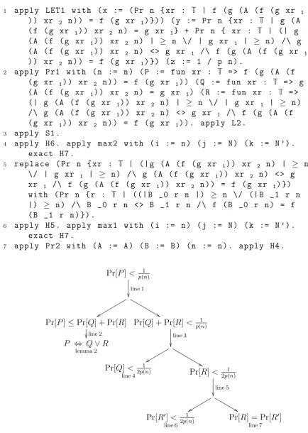
Proof Let us focus on the last part of the proof (paragraph 3 of the traditional proof) because is the more difficult one. At this point of the proof

• we have N and N0, and took n > N00 = max(N, N0), which is such that Pr[Q] < 1/(2p(n)) and Pr[R0] < 1/(2p(n)) (paragraph 2 of the traditional proof);

• we are about to prove Pr[P] ≤ Pr[Q] + Pr[R] and Pr[Q] + Pr[R] < 1/p(n) (paragraph 3 of the traditional proof).

(12)

1 a p p l y LET1 with ( x := ( Pr n { xr : T | f ( g ( A ( f ( g xr 1 ) ) xr 2 n ) ) = f ( g xr 1) }) ) ( y := Pr n { xr : T | g ( A ( f ( g xr 1) ) xr 2 n ) = g xr 1} + Pr n { xr : T | (| g ( A ( f ( g xr 1) ) xr 2 n ) | ≥ n \/ | g xr 1 | ≥ n ) /\ g ( A ( f ( g xr 1) ) xr 2 n ) <> g xr 1 /\ f ( g ( A ( f ( g xr 1 ) ) xr 2 n ) ) = f ( g xr 1) }) ( z := 1 / p n ) .

2 a p p l y Pr1 with ( n := n ) ( P := fun xr : T = > f ( g ( A ( f ( g xr 1) ) xr 2 n ) ) = f ( g xr 1) ) ( Q := fun xr : T = > g ( A ( f ( g xr 1) ) xr 2 n ) = g xr 1) ( R := fun xr : T = > (| g ( A ( f ( g xr 1) ) xr 2 n ) | ≥ n \/ | g xr 1 | ≥ n ) /\ g ( A ( f ( g xr 1) ) xr 2 n ) <> g xr 1 /\ f ( g ( A ( f ( g xr 1) ) xr 2 n ) ) = f ( g xr 1) ) . a p p l y L2 .

3 a p p l y S1 .

4 a p p l y H6 . a p p l y max2 with ( i := n ) ( j := N ) ( k := N ’) .

e x a c t H7 .

5 r e p l a c e ( Pr n { xr : T | (| g ( A ( f ( g xr 1) ) xr 2 n ) | ≥ n \/ | g xr 1 | ≥ n ) /\ g ( A ( f ( g xr 1) ) xr 2 n ) <> g xr 1 /\ f ( g ( A ( f ( g xr 1) ) xr 2 n ) ) = f ( g xr 1) }) with ( Pr n { r : T | ((| B _0 r n |) ≥ n \/ (| B _1 r n |) ≥ n ) /\ B _0 r n <> B _1 r n /\ f ( B _0 r n ) = f ( B _1 r n ) }) .

6 a p p l y H5 . a p p l y max1 with ( i := n ) ( j := N ) ( k := N ’) . e x a c t H7 .

7 a p p l y Pr2 with ( A := A ) ( B := B ) ( n := n ) . a p p l y H4 .

Pr[P]< 1

p(n)

line 1

x

x &&

Pr[P]≤Pr[Q] + Pr[R]

line 2

Pr[Q] + Pr[R]< _p₍1_n₎

line 3

P ⇔ Q∨R

lemma 2

x

x _&_&

Pr[Q]< ₂_p1₍_n₎

line 4 Pr[R]<

1 2p(n)

line 5

x

x &&

Pr[R0]< ₂_p1₍_n₎

line 6

Pr[R] = Pr[R0]

line 7

(13)

Annex

1 (* L A N G U A G E *)

2 P a r a m e t e r R: Set . (* Real n u m b e r s *)

3 P a r a m e t e r N : Set . (* N a t u r a l n u m b e r s *)

4 P a r a m e t e r T : Set . (* Two - star , that is , 2* = {0 ,1}* *)

5 P a r a m e t e r P : (T -> T) -> Prop . (* C o m p u t a b l e in p o l y n o m i a l time ( on the l e n g t h of the i n p u t ) *)

6 P a r a m e t e r NP : (T -> N -> T) -> Prop . (* R a n d o m i s e d

p o l y n o m i a l time a l g o r i t h m s ( on the l e n g t h of the i n p u t ) *)

7 P a r a m e t e r NP’ : (T -> T -> N -> T) -> Prop . (*

R a n d o m i s e d p o l y n o m i a l time a l g o r i t h m s ( on the l e n g t h of the i n p u t ) *)

8 P a r a m e t e r NP’’ : (N -> T -> N -> T) -> Prop . (*

R a n d o m i s e d p o l y n o m i a l time a l g o r i t h m s ( on the l e n g t h of the i n p u t ) *)

9 P a r a m e t e r Pr : N -> Set -> R. (* P r o b a b i l i t y p r e d i c a t e *)

10 P a r a m e t e r Π : (N -> N) -> Prop . (* P o s i t i v e p o l y n o m i a l s *)

11 P a r a m e t e r GT : N -> N -> Prop . (* " G r e a t e r than " b e t w e e n

n a t u r a l n u m b e r s *)

12 N o t a t i o n " x ’ > ’ y " := ( GT x y ) . (* " >" for " g r e a t e r

than " *)

13 P a r a m e t e r GET : N -> N -> Prop . (* " G r e a t e r than or e q u a l to " b e t w e e n n a t u r a l n u m b e r s *)

14 N o t a t i o n " x ’≥’ y " := ( GET x y ) ( at l e v e l 70) . (* "≥"

for " g r e a t e r than or e q u a l to " *)

15 P a r a m e t e r LT : R -> R -> Prop . (* " Less than " b e t w e e n

real n u m b e r s *)

16 N o t a t i o n " x ’ < ’ y " := ( LT x y ) ( at l e v e l 70) . (* " <" for " less than " *)

17 P a r a m e t e r LET : R -> R -> Prop . (* " Less than or e q u a l

to " b e t w e e n real n u m b e r s *)

18 N o t a t i o n " x ’≤’ y " := ( LET x y ) ( at l e v e l 70) . (* "≤"

for " less than or e q u a l to " *)

19 P a r a m e t e r I : N -> R. (* " I n v e r s i o n of " a n a t u r a l n u m b e r *)

20 N o t a t i o n "1 / x " := ( I x ) ( at l e v e l 60) . (* "1 /" for

" i n v e r s e of " *)

21 P a r a m e t e r S : R -> R -> R. (* " sum of " real n u m b e r s *)

22 N o t a t i o n " x + y " := ( S x y ) . (* "+" for " sum of " *)

23 P a r a m e t e r D : N -> N. (* " D o u b l e of " a n a t u r a l n u m b e r *)

24 N o t a t i o n "2 x " := ( D x ) ( at l e v e l 70) . (* "2" for

(14)

25 P a r a m e t e r max : N -> N -> N. (* " M a x i m u m of " n a t u r a l n u m b e r s *)

26 P a r a m e t e r p_1 : T -> T. (* F i r s t and s e c o n d p r o j e c t s of

a b i n a r y s t r i n g r e g a r d e d as an ... *)

27 P a r a m e t e r p_2 : T -> T. (* ... o r d e r e d pair of b i n a r y

s t r i n g s u n d e r some s u i t a b l e e n c o d i n g *)

28 N o t a t i o n " x 1" := ( p_1 x ) ( at l e v e l 1) . (* "1" for " f i r s t p r o j e c t i o n " *)

29 N o t a t i o n " x 2" := ( p_2 x ) ( at l e v e l 1) . (* "2" for " f i r s t p r o j e c t i o n " *)

30 P a r a m e t e r L : T -> N. (* " L e n g t h of " a s t r i n g *)

31 N o t a t i o n "| x |" := ( L x ) ( at l e v e l 70) . (* "| |" for

" l e n g t h of " *)

32 P a r a m e t e r _0 _1 : N. (* N a t u r a l n u m b e r s zero and one *)

33 P a r a m e t e r f g : T -> T. (* F u n c t i o n s f and g *)

34

35 (* A X I O M S *)

36 R e q u i r e I m p o r t Coq . L o g i c . C l a s s i c a l _ P r o p . (* C l a s s i c a l

l o g i c *)

37 A x i o m P1 : f o r a l l g : T -> T, P g -> P ( fun xr : T = > g

xr 1) . (* g ( xr1) is c o m p u t a b l e in p o l y n o m i a l time *)

38 A x i o m NP1 : f o r a l l ( A : T -> N -> T) ( g : T -> T) , (NP A -> P g -> e x i s t s B : N -> T -> N -> T, NP’’ B /\

f o r a l l ( x : T) ( n : N) , B _0 x n = A x n /\ B _1 x n = g x ) . (* A l g o r i t h m d e f i n i t i o n by c a s e s B (0 , x ) = A ( x ) , B (1 , x ) = g ( x ) *)

39 A x i o m NP2 : f o r a l l ( A : T -> T -> N -> T) ( f g : T -> T

) , NP’ A -> P f -> P g -> NP ( fun ( xr : T) ( n : N) = > g ( A ( f ( g xr 1) ) xr 2 n ) ) . (* g ( A ( f ( g ( xr1) ) , xr2, n ) ) is a r a n d o m i s e d p o l y n o m i a l time a l g o r i t h m *)

40 A x i o m NP3 : f o r a l l ( A : T -> T -> N -> T) ( f : T -> T) , NP’ A -> P f -> NP’ ( fun ( x y : T) ( n : N) = > A ( f x ) y n ) . (* A ( f ( x ) ,y , n ) is a r a n d o m i s e d p o l y n o m i a l time a l g o r i t h m *)

41 A x i o m Π1 : f o r a l l p : N -> N, (Π p -> Π ( fun n : N = > 2

p n ) ) . (* The d o u b l e of a p o s i t i v e p o l y n o m i a l is a p o s i t i v e p o l y n o m i a l *)

42 A x i o m max1 : f o r a l l i j k : N, i > max j k -> i > j . (*

i > max ( j , k ) -> i > j *)

43 A x i o m max2 : f o r a l l i j k : N, i > max j k -> i > k . (* i > max ( j , k ) -> i > k *)

44 A x i o m S1 : f o r a l l ( n : N) ( p : N -> N) ( X Y : R) , X < 1

/ (2 p n ) -> Y < 1 / (2 p n ) -> ( X + Y ) < 1 / p n . (* E s s e n t i a l l y x , y < 1/2 -> x + y < 1 *)

45 A x i o m GET1 : f o r a l l x y z : N, x ≥ y -> y ≥ z -> x ≥ z .

(15)

46 A x i o m LET1 : f o r a l l x y z : R, x ≤ y -> y < z -> x < z . (* M i x e d t r a n s i t i v i t y of ≤ and < *)

47 A x i o m Pr1 : f o r a l l ( n : N) ( P Q R : T -> Prop ) , ( f o r a l l

x : T, | x 1 | ≥ n -> | x 2 | ≥ n -> ( P x < - > Q x \/ R x ) ) -> Pr n { x : T | P x } ≤ Pr n { x : T | Q x } + Pr n { x : T | R x }. (* E s s e n t i a l l y Pr [ A U B ] ≤ Pr A + Pr B *)

48 A x i o m Pr2 : f o r a l l ( A : T -> T -> N -> T) ( B : N -> T ->

N -> T) ( n : N) , ( f o r a l l ( x : T) ( n : N) , B _0 x n = g ( A ( f ( g x 1) ) x 2 n ) /\ B _1 x n = g x 1) -> Pr n { r : T | (| B _0 r n | ≥ n \/ | B _1 r n | ≥ n ) /\ B _0 r n <> B _1 r n /\ f ( B _0 r n ) = f ( B _1 r n ) } = ( Pr n { xr : T | (| g ( A ( f ( g xr 1) ) xr 2 n ) | ≥ n \/ | g xr 1 | ≥ n ) /\ g ( A ( f ( g xr 1) ) xr 2 n ) <> g xr 1 /\ f ( g ( A ( f ( g xr 1) ) xr 2 n ) ) = f ( g xr 1) }) . (* E s s e n t i a l l y A = B -> Pr A = Pr B *)

49 A x i o m F1 : P f . (* f is ... *)

50 A x i o m F2 : f o r a l l A : N -> T -> N -> T, (NP’’ A ->

f o r a l l p : N -> N, (Π p -> e x i s t s N : N, f o r a l l n : N , ( n > N -> Pr n { r : T | (| A _0 r n | ≥ n \/ | A _1 r n | ≥ n ) /\ A _0 r n <> A _1 r n /\ f ( A _0 r n ) = f ( A _1 r n ) } < (1 / p n ) ) ) ) . (*

... c o l l i s i o n - r e s i s t a n t *)

51 A x i o m G1 : P g . (* g is ... *)

52 A x i o m G2 : f o r a l l A : T -> T -> N -> T, (NP’ A -> f o r a l l p : N -> N, (Π p -> e x i s t s N : N, f o r a l l n : N, ( n >

N -> Pr n { xr : T | g ( A ( g xr 1) xr 2 n ) = g xr 1} < (1 / p n ) ) ) ) . (* ... one - way *)

53 A x i o m G3 : f o r a l l x : T, | g x | ≥ | x |. (* g is

length - n o n d e c r e a s i n g *)

54

55 (* LEMMAS , T H E O R E M AND P R O O F S *)

56 L e m m a L1 : f o r a l l ( A : T -> T -> N -> T) , NP’ A ->

e x i s t s ( B : N -> T -> N -> T) , NP’’ B /\ f o r a l l ( xr : T) ( n : N) , B _0 xr n = g ( A ( f ( g xr 1) ) xr 2 n ) /\ B

_1 xr n = g xr 1.

57

58 P r o o f .

59 i n t r o s A H1 .

60 d e s t r u c t NP1 with ( A := fun ( xr : T) ( n : N) = > g ( A ( f ( g xr 1) ) xr 2 n ) ) ( g := fun ( xr : T) = > g xr 1) as [ B [ H2 H3 ]].

61 a p p l y NP2 with ( A := A ) . e x a c t H1 .

62 e x a c t F1 .

63 e x a c t G1 .

(16)

65 e x i s t s B .

66 s p l i t .

67 e x a c t H2 .

68 e x a c t H3 .

69 Qed .

70

71 L e m m a L2 : f o r a l l ( A : T -> T -> N -> T) ( n : N) ( xr : T ) , | xr 1 | ≥ n -> | xr 2 | ≥ n -> ( f ( g ( A ( f ( g xr 1) ) xr 2 n ) ) = f ( g xr 1) < - > g ( A ( f ( g xr 1) ) xr 2 n ) = g xr 1

\/ (| g ( A ( f ( g xr 1) ) xr 2 n ) | ≥ n \/ | g xr 1 | ≥ n ) /\ g ( A ( f ( g xr 1) ) xr 2 n ) <> g xr 1 /\ f ( g ( A ( f ( g xr 1) ) xr 2 n ) ) = f ( g xr 1) ) .

72

73 P r o o f .

74 i n t r o s A n xr H1 H2 .

75 s p l i t .

76 i n t r o H3 .

77 d e s t r u c t c l a s s i c with ( P := g ( A ( f ( g xr 1) ) xr 2 n ) = g xr 1) as [ H4 | H5 ].

78 left . e x a c t H4 .

79 r i g h t . s p l i t .

80 r i g h t . a p p l y GET1 with ( x := | g xr 1 |) ( y := | xr 1 |) ( z := n ) .

81 a p p l y G3 .

82 e x a c t H1 .

83 s p l i t .

84 e x a c t H5 .

85 e x a c t H3 .

86 i n t r o s [ H6 | [ H7 [ H8 H9 ]]].

87 r e p l a c e ( g ( A ( f ( g xr 1) ) xr 2 n ) ) with ( g xr 1) . r e f l e x i v i t y .

88 e x a c t H9 .

89 Qed .

90

91 T h e o r e m T1 : f o r a l l A : T -> T -> N -> T, (NP’ A ->

f o r a l l p : N -> N, (Π p -> e x i s t s N : N, f o r a l l n : N , ( n > N -> Pr n { xr : T | f ( g ( A ( f ( g xr 1) ) xr 2 n ) ) = f ( g xr 1) } < (1 / p n ) ) ) ) .

92

93 P r o o f .

94 i n t r o s A H1 p H2 .

95 (* I n t r o d u c i n g B such that B (0 , xr , n ) =

g ( A ( f ( g ( xr1) ) ) , xr2, n ) and B (1 , xr , n ) = g ( xr1) *)

96 d e s t r u c t L1 with ( A := A ) as [ B [ H3 H4 ]].

97 e x a c t H1 .

(17)

99 d e s t r u c t F2 with ( A := B ) ( p := fun n : N = > 2 p n ) as [ N H5 ].

100 e x a c t H3 .

101 a p p l y Π1 with ( p := p ) . e x a c t H2 .

102 (* G e t t i n g N2 from one - w a y n e s s of g *)

103 d e s t r u c t G2 with ( A := fun ( x y : T) ( n : N) = > A ( f

x ) y n ) ( p := fun n : N = > 2 p n ) as [ N ’ H6 ].

104 a p p l y NP3 with ( A := A ) . e x a c t H1 . e x a c t F1 .

105 a p p l y Π1 with ( p := p ) . e x a c t H2 .

106 (* T a k i n g N = max ( N1 , N2 ) *)

107 e x i s t s ( max N N ’) .

108 i n t r o s n H7 .

109 (* S p l i t i n g a p r o b a b i l i t y into the sum of two p r o b a b i l i t i e s *)

110 a p p l y LET1 with ( x := ( Pr n { xr : T | f ( g ( A ( f ( g xr

1) ) xr 2 n ) ) = f ( g xr 1) }) ) ( y := Pr n { xr : T | g ( A ( f ( g xr 1) ) xr 2 n ) = g xr 1} + Pr n { xr : T | (| g ( A ( f ( g xr 1) ) xr 2 n ) | ≥ n \/ | g xr 1 | ≥ n ) /\ g ( A ( f ( g xr 1) ) xr 2 n ) <> g xr 1 /\ f ( g ( A ( f ( g xr 1) ) xr 2 n ) ) = f ( g xr 1) }) ( z := 1 / p n ) .

111 a p p l y Pr1 with ( n := n ) ( P := fun xr : T = > f ( g ( A

( f ( g xr 1) ) xr 2 n ) ) = f ( g xr 1) ) ( Q := fun xr : T = > g ( A ( f ( g xr 1) ) xr 2 n ) = g xr 1) ( R := fun xr : T = > (| g ( A ( f ( g xr 1) ) xr 2 n ) | ≥ n \/ | g xr 1 | ≥ n ) /\ g ( A ( f ( g xr 1) ) xr 2 n ) <> g xr 1

/\ f ( g ( A ( f ( g xr 1) ) xr 2 n ) ) = f ( g xr 1) ) . a p p l y L2 .

112 a p p l y S1 .

113 a p p l y H6 . a p p l y max2 with ( i := n ) ( j := N ) ( k :=

N ’) . e x a c t H7 .

114 r e p l a c e ( Pr n { xr : T | (| g ( A ( f ( g xr 1) ) xr 2 n ) | ≥ n \/ | g xr 1 | ≥ n ) /\ g ( A ( f ( g xr 1) ) xr

2 n ) <> g xr 1 /\ f ( g ( A ( f ( g xr 1) ) xr 2 n ) ) = f ( g xr 1) }) with ( Pr n { r : T | (| B _0 r n | ≥ n \/ | B _1 r n | ≥ n ) /\ B _0 r n <> B _1 r n /\ f ( B _0 r n ) = f ( B _1 r n ) }) .

115 a p p l y H5 . a p p l y max1 with ( i := n ) ( j := N ) ( k := N ’) . e x a c t H7 .

116 a p p l y Pr2 with ( A := A ) ( B := B ) ( n := n ) . a p p l y

H4 .

117 Qed .

References

(18)

[2] Shafi Goldwasser and Mihir Bellare. Lecture notes on cryptography. http://cseweb.ucsd.edu/ mihir/papers/gb.pdf.

[3] Rafael Pass and Chin Isradisaikul. Cryptography. https://www.cs.cornell.edu/courses/cs6830/2009fa/.