DOI: 10.1534/genetics.107.072009
Fixation Probabilities When Generation Times Are Variable:
The Burst–Death Model
J. E. Hubbarde,
1G. Wild and L. M. Wahl
Department of Applied Mathematics, University of Western Ontario, London, Ontario N6A 5B7, Canada
Manuscript received February 12, 2007 Accepted for publication May 1, 2007
ABSTRACT
Estimating the fixation probability of a beneficial mutation has a rich history in theoretical population genetics. Typically, to attain mathematical tractability, we assume that generation times are fixed, while the number of offspring per individual is stochastic. However, fixation probabilities are extremely sensitive to these assumptions regarding life history. In this article, we compute the fixation probability for a ‘‘burst– death’’ life-history model. The model assumes that generation times are exponentially distributed, but the number of offspring per individual is constant. We estimate the fixation probability for populations of constant size and for populations that grow exponentially between periodic population bottlenecks. We find that the fixation probability is, in general, substantially lower in the burst–death model than in classical models. We also note striking qualitative differences between the fates of beneficial mutations that increase burst size and mutations that increase the burst rate. In particular, once the burst size is sufficiently large relative to the wild type, the burst–death model predicts that fixation probability de-pends only on burst rate.
E
STIMATING the fixation probability of an initially rare beneficial mutation is fundamental to our understanding of adaptation. Such estimates are crit-ical to studies of evolution under controlled laboratory conditions and are also essential for predicting the rate of adaptation of natural populations—for example, the rate of adaptation in response to environmental change or the rate of emergence of novel, or drug-resistant, pathogens.To date, a considerable body of theoretical literature has been devoted to this question, beginning with classic articles such as Fisher(1922) and Haldane(1927). To
attain mathematical tractability, these approaches have necessarily imposed a number of simplifying assump-tions. In particular, the life-history models of classical popu-lation genetics typically assume that generation times are fixed, with no death between generations. However, recent work in our group (e.g., Wahl and DeHaan
2004) has emphasized that fixation probabilities are extremely sensitive to the underlying life-history model. The work described here is motivated, in part, by the extensive and important body of literature regarding the experimental evolution of lytic viruses (e.g., Bull et al.
1997, 2000; Burchand Chao1999, 2000; Wichmanet al.
1999; Sanjua´ net al. 2005; Manrubiaet al. 2005). For lytic
bacteriophages in particular, each ‘‘generation’’ time consists of an attachment time, during which the viral
particle ‘‘searches’’ for a cell to infect, and alysis time, the time between attachment and lysis, during which phage accumulate within the infected cell. Although the lysis (or ‘‘phage-accumulation’’) time may be tightly regu-lated, attachment times are well modeled by a first-order process;i.e., they are exponentially distributed (Abedon
et al. 2001).
When attachment times are very short, the standard assumption of fixed generation times is clearly valid. In this article, however, we develop a life-history model in which generation times vary. In particular, we treat the case when ‘‘death’’ occurs at a constant rate, and thus generation times (or, more correctly, lifetimes) are exponentially distributed. This may be an appropriate model for estimating fixation probabilities for lytic vi-ruses, particularly when the attachment time is long compared to the phage-accumulation time, and may also be applied to other natural and experimental pop-ulations where generation times vary widely.
A BURST–DEATH LIFE-HISTORY MODEL
We have developed the ‘‘burst–death’’ life-history model in analogy to the well-studied birth–death process. There are two ways, intuitively, to derive this model. First, we can consider an individual with a constant probability of death,MDt, in any small interval of time,Dt. An example of such a process is the clearance of free virus or bacteria from a chemostat, or, more generally, any failure of a virion to infect a new cell. We also note thatMmay be zero, a case we treat explicitly in the sections that follow. While alive, 1Corresponding author:Department of Applied Mathematics, Middlesex
College, Room 255, University of Western Ontario, London, ON N6A 5B7, Canada. E-mail: [email protected]
the individual has a constant probability of reproducing, LDt, in time interval Dt. These assumptions yield an exponential distribution of lifetimes. Note, however, that the latter assumption also implies that the time until reproduction doesnotdepend on the age of the organism. The assumption that the probability of reproducing is constant for any age is the main limitation of the burst– death model and is clearly an avenue for future work. We return to this idea in thediscussion.
If the individual reproduces, a ‘‘burst’’ of a fixed number of offspring is produced. In analogy to a linear birth–death process, we can either assume that the par-ent organism survives whenBnew offspring enter the population or assume that the parent dies when the offspring are produced, but B 1 1 offspring are pro-duced. These are mathematically equivalent since the age of the organism does not matter.
A second way to derive the same model is to imagine that each individual has a lifetime drawn from an ex-ponential distribution. At the end of its life, the indi-vidual reproduces, producing either zero or B 1 1 offspring. Although this second formulation may seem somewhat different from the first, for the purposes of computing fixation probabilities they are precisely equiv-alent. In particular, we have equivalence when lifetimes (generation times) in the second model are drawn from an exponential distribution with mean 1/(M1L), and the probability of having zero offspring is given byM/ (M1L). We note that whileMandLare positive real numbers,Bis constrained to be a positive integer.
In the results anddiscussion to follow, we often
compare the predictions of the burst–death model to the predictions of what we refer to as the ‘‘classic’’ model (Fisher1922; Haldane1927), which has the following
assumptions: (1) generation times are fixed, (2) there is no death between generations, (3) the number of off-spring produced by each individual follows a Poisson distribution, and (4) beneficial mutations confer an increased average number of offspring. Thus in the clas-sic model, lifetimes are fixed but stochasticity occurs via the Poisson distribution of offspring, whereas in the burst–death model, lifetimes are stochastic but the number of offspring is fixed.
Selective advantage: Suppose that the wild-type pop-ulation consists of individuals as described above, with constant burst rateL, constant death rateM, and burst sizeB. A population of sizeN0at time zero would then
have total expected sizeN0e(BLM)tat timet. We initially
restrict our attention to the case whenBL¼M; other-wise the population is on average growing or decaying exponentially, and the fixation probability is of little in-terest. In the next section, we relax this assumption and introduce population bottlenecks.
Analogously, an individual with a beneficial mutation has burst ratel, death ratem, and burst sizeb. Since the mutant reproduces more effectively than the wild type, we might have, for example,b¼B1DB, whereb,B, and
DBare all integers. To find the selective advantage,s, of such a mutant, recall that in standard population ge-netics models, a beneficial mutation increases the ex-pected number of offspring in a generation fromWto W(11 s). In this case, however, the expected number of offspring in a mean wild-type generation time of 1/ (L1M) increases from
W ¼eðBLMÞ=ðL1MÞ
to
Wð11sÞ ¼eððB1DBÞLMÞ=ðL1MÞ:
Solving, we find that the classically defined selective advantage,s, is given by
s¼eDBL=ðL1MÞ1; forb¼B1DB: ð1Þ
Note that Equation 1 applies only when the beneficial mutation confers an increased burst size,b¼B1DB. A similar expression can likewise be derived forswhen the mutation confers an increased burst rate,l.L, or de-creased death rate, m, M. For a mutation with burst ratel¼L(11d), for example, we find that
s¼eBLd=ðL1MÞ1; forl¼Lð11dÞ: ð2Þ
The selective advantagesthus depends on the wild-type burst size, as well as on the wild-type burst and death rates (this factor becomes important in interpreting Figure 2 in theresults).
Fixation and extinction probabilities: We use X to denote the extinction probability, the probability that a lineage carrying a beneficial mutant is ultimately lost due to stochastic fluctuations in the size of the lineage. Throughout this article, we also use p to denote the complement of this probability, p¼1X. In reality, a beneficial mutation could also be driven to extinction through clonal interference (Gerrishand Lenski1998)
or could fix through quasispecies interactions (Wilke
2003); we ignore both of these possibilities. Thus tech-nically, p does not give the fixation probability; we nonetheless use this parameter extensively (for exam-ple, in the figures) as shorthand for 1X.
Linear birth–death process:Whenb¼1, the burst– death model yields the classic linear birth–death pro-cess, which has been studied in depth (Taylor and
Karlin1998). It is well known that the extinction
pro-bability for a birth–death process is one ifm $ l, which can occur only ifsis negative. The more interesting case occurs for positives; in this case we havem,land the extinction probability is given byX¼m/l(Grimmett
and Stirzaker2001).
offspring, but each of these lineages goes extinct. This yields
X ¼ m
m1l1 l m1lX
b11; ð3Þ
wherem/(m1l) gives the probability that an individual dies before bursting. Solving this equation forX, we find that as long asb.4 or 5,Xm/(m1l). This result is quite straightforward from a mathematical point of view, but is somewhat surprising from a biological per-spective. In particular, we would typically expect that ass grows very large, the fixation probability should ap-proach one. Here, when either m decreases or l in-creases, this remains true. However, when s increases through an increase in burst size,b, the fixation prob-ability approaches a plateau,l/(m1l), which may be much less than one. In fact, this maximum value ofpis equal to the probability of bursting before dying. This feature comes up again in theresults(Figures 1 and 2).
POPULATION BOTTLENECKS
A limitation of the burst–death model is that unless the overall rate at which offspring are produced exactly balances the death rate, BL ¼M, the population will grow exponentially without bound or decay exponen-tially to extinction. We extend this model, relaxing the assumption that BL is precisely balanced by M. In particular, we explore the case whenBL.M, such that the population on average experiences sustained inter-vals of growth. We then assume that these growth in-tervals are balanced by population bottlenecks that reduce the population to its initial size.
Once again, we use the simplest possible model to allow tractability. We assume, as in previous work (Wahl
and Gerrish2001; Heffernanand Wahl2002), that
the wild-type population grows forttime units, at which point a population bottleneck occurs. Each individual in the population independently survives the bottleneck with probabilityD, and the process repeats. Assuming that, on average, the bottleneck restores the population to its size at the start of the growth phase, we find thatD must be given byD¼e(BLM)t.
To solve for the fixation or extinction probability in this case is somewhat more difficult. Our approach is as follows. We first consider a beneficial mutation that ex-ists as a single copy at the beginning of a growth phase. We then derive an implicit equation for G(x, t), the probability generating function (pgf) that describes the number of offspring in this mutant lineage at the end of the growth phase. Each individual in the population survives the bottleneck with probabilityDand does not survive with probability 1D; thus the pgf for the bot-tleneck process is given byH(x)¼1D1Dx. Overall, then, the pgf for the number of individuals in the mu-tant lineage after one cycle of growth and sampling is
given byF(x)¼G(H(x),t). Finally, the extinction pro-bability for a single lineage present at the start of a growth phase, which we denoteX0, is given by the fixed
point of this pgf,i.e., by the solution to
X0 ¼Gð1D1DX0;tÞ: ð4Þ The extinction probability for mutations that first occur at other times during the growth phase can be computed very simply fromX0, as described in a later section. The
difficult step in this approach is deriving, and then solv-ing, an implicit equation forG(x,t).
Birth–death model with bottlenecks: For the linear birth–death model (b¼1), the probability generating functionG(x,t) is well known and is typically found as the solution to the following partial differential equa-tion (PDE), which can be derived from first principles in a straightforward way (Grimmettand Stirzaker2001):
@G
@t ¼ ðlx
2 ðl1mÞx1mÞ@G
@x; forb¼1:
This is a PDE of the Lagrange type and can be solved us-ing the partial fraction expansion of the auxiliary equa-tion and the usual boundary condiequa-tions (G(x, 0)¼x, G(1,t)¼1), to give
Gðx;tÞ ¼me
ðlmÞtðx1Þ lx1m
leðlmÞtðx1Þ lx1m; forb¼1
(Grimmettand Stirzaker2001). The fixed point of
G(1D1Dx,t) gives the extinction probability,X0, and
can be found exactly:
X0 ¼
meðlmÞtl1ðlmÞ=D leðlmÞtl :
WhileX0explicitly depends on the life-history
parame-ters of the mutant (landm), the analogous parameters for the wild type (LandM) also affectX0through the
constantD.
Burst–death model with bottlenecks: For b.1, we can derive the following PDE from first principles, as de-scribed in detail in theappendix:
@G
@t ¼ ðlx
b11 ðl1mÞx1mÞ@G
@x: ð5Þ
Once again this is a PDE of the Lagrange type and can be solved in an analogous way to theb ¼1 case. The details of this solution are provided in the appendix,
which demonstrates thatG(x,t) is given by the value ofy on½0, 1that satisfies
0¼wY i
ðyxiÞLi y11;
where the xi are the b roots of the polynomiallxb1 lxb11. . .1lxm, and the formulas forwand for the
This solution is inelegant, but numerically tractable even for very large values ofb, for example,b¼100.
Pure burst model with bottlenecks: A more elegant description ofG(x,t) can be found for the case when
m¼ 0, which we call a pure burst processwith periodic bottlenecks. In this simpler case, we can use a result from the study of continuous-time branching processes; for a very clear derivation, see Allen(2003, p. 240). This
result holds when individuals in the population have exponentially distributed lifetimes with mean 1/l, and at the end of a lifetime produce a random number of offspring according to the probability generating func-tionf(x). In this case, if a lineage begins with a single individual at time zero, the pgf describing the total number of individuals in a lineage at timet,P(x,t), must satisfy
@Pðx;tÞ
@t ¼ l½Pðx;tÞ fðPðx;tÞÞ: ð6Þ
This formulation yields the pure burst process whenf(x) is given byf(x)¼xb11; that is, lifetimes are exponentially
distributed with mean 1/l, and each individual has exactlyb11 offspring.
Substituting f(x) into Equation 6, we obtain the solution
Pðx;tÞ ¼ ð11ebltðxb1ÞÞ1=b:
Once again, if regular bottlenecks are imposed every
t-time units, the extinction probability for a novel bene-ficial mutation that first occurs at time zero, just after a bottleneck, is given by the solution to
X0 ¼Pð1D1DX0;tÞ: ð7Þ
Mutations that occur at timetduring growth:We now consider the case of mutations that occur at timet dur-ing a growth phase, with 0,t# t. In this case, the line-age hastttime units to grow before facing the first bottleneck. ThusG(x,tt) gives the pgf describing the number of individuals in the lineage just before the first bottleneck, andG(1D1Dx,tt) gives the pgf for the number of individuals in the lineage after the first bot-tleneck. Thus, ifpidenotes the probability that there are iindividuals in the lineage just after the first bottleneck, we could write
Gð1D1Dx;ttÞ ¼p01p1x1p2x21. . .: Now consider the extinction probability,Xt, for a lineage that first appears as a single copy at timet. If this lineage has no survivors after the first bottleneck, the lineage is extinct; this occurs with probabilityp0. Or, a single
indi-vidual could survive the first bottleneck, with probability p1, but that lineage could go extinct, with probabilityX0,
as derived in Equation 4. Or, two individuals could sur-vive the first bottleneck (probability p2), but both of
those lineages independently go extinct, with
probabil-ity (X0)2. This line of reasoning leads us to the following
result:
Xt¼p01p1X01p2ðX0Þ21. . .
¼Gð1D1DX0;ttÞ; ð8Þ where in the most general case X0 is the solution to
Equation 4 andG(x,t) is the solution to Equation 5.
RESULTS
Here we illustrate the fixation probability as obtained through the numerical solution of the equations pre-sented in the previous section. To verify this analytical and numerical work, we also performed extensive Monte Carlo (individual-based) simulation. In the simulations, we start with a single individual with a beneficial mu-tation, whose burst time is drawn from an exponential distribution, and who faces a constant probability of death, at ratem. If the individual survives until the burst time,b11 offspring are produced. The offspring each behave independently, dying or bursting as described above, with independently drawn burst times. At timet, each individual in the population survives the bottle-neck with probabilityD. This process is repeated until the mutant population either becomes extinct or grows to a size sufficient that the probability of future ex-tinction is negligible. This procedure constitutes a sin-gle ‘‘run’’ of the Monte Carlo simulation; we typically use 100,000 runs to estimate fixation probabilities. In all cases, we found that the simulation results were indistin-guishable from the numerical results reported below.
Figure 1 illustrates the fixation probability vs. the selective advantage,s, as defined in Equations 1 and 2, for a burst–death model with a constant population size. In this case there are no population bottlenecks, and the rate at which new individuals are produced,BL, must be exactly balanced by the death rate,M. In Figure 1, we have setL¼1 and increased the wild-type burst size,B, from 1 to 100 (labels on the right). The fixation prob-ability is given for beneficial mutations that increase the burst size to give the selective advantage as described in Equation 1. We see that for populations with larger wild-type burst sizes, and thus correspondingly large death rates, the fixation probability is dramatically reduced, even for large values ofs.
burst size,b, this probability remains fixed, and results in an upper bound onp.
For comparison, the thick line in Figure 1 shows the classic fixation probability obtained in a constant
pop-ulation size, under the assumptions for the classic case that we enumerated earlier. Herepapproaches one ass grows large, as expected. This is because assgrows large, the mean of the Poisson distribution of offspring grows large, and the probability of having zero offspring be-comes negligible. We also note, as an aside, that the classic approach yields the same values ofpfor any value ofBoffspring per generation. This is because a Poisson distribution with meanB, randomly sampled with prob-ability 1/B (such that only one offspring survives on average, maintaining a constant population size) gives the same Poisson distribution, with mean one, for any value ofB.
In Figure 1b, we again explore the case without pop-ulation bottlenecks (M¼BL) and plot the fixation prob-ability for beneficial mutations that increase the burst rate,l¼L(11d). In this case, the probability of dying before bursting, m/(m 1 l), approaches zero as l
increases, and thuspapproaches one, albeit only when sis very large (not shown). We also note that pis very different, at the same value ofs, between Figure 1a and 1b; in the burst–death model, the fixation probability is extremely sensitive to the mechanismof the selective advantage. In a constant population, increases in burst rate are more likely to fix than increases in burst size.
In Figures 2–4, we explore fixation probabilities for cases when BL$ M, and thus population bottlenecks must be imposed, everyt-time units, to restrict popula-tion growth. For all of these figures, we have assumed that the wild-type population has burst rateL¼1 and burst sizeB¼100. The beneficial mutation first occurs in a single copy at time zero (we vary this in Figure 4). The death rate, M, varies between zero, a pure burst process, andM¼BL, a constant population size.
We note that despite these differences inM, the over-all probability that a single individual will die, over one cycle of growth and sampling, is constant. At M ¼0, however, all death occurs at the bottleneck, whereas at M¼BL, all death occursbetweenbottlenecks. This is be-cause the latter case represents the limit at whichD¼1, and effectively bottlenecks no longer occur. Thus de-creasingMfromBLto zero can be thought of as gradually imposing more severe bottlenecks, while concomitantly reducing the death rate between bottlenecks.
Also in Figures 2–4, we typically show results fort¼
0.3. Since the mean lifetime is given by 1/L¼1, this bottleneck time may appear short compared to exper-imental practice. However, when the burst size is 100, and there is no delay between attachment and lysis (as our model assumes), the wild-type population size grows extremely quickly. For example, at the highest death rate, M¼BL, the bottleneck ratio,D, is one. However consider the next highest death rate,M¼BL/2. Here the virus is cleared 50 times faster than the burst rate, yet att¼0.3 the bottleneck ratio is given byD¼exp((BL
BL/2)t)107, and this becomes even more severe for
lower death rates. Thus t¼0.3 represents a relatively Figure1.—Fixation probabilities in a population of
‘‘long’’ bottleneck time, and we explore shorter times (less severe bottleneck ratios) in Figures 3 and 4c.
In Figure 2, we illustrate the behavior of p with in-creases in burst size (Figure 2a) and burst rate (Figure 2b). We find that as the wild-type death rate,M, increases, the fixation probability decreases. Thus p decreases even though the bottlenecks are becominglesssevere. This result critically depends on the time at which the beneficial mutation first occurs, however; in Figure 2 we
consider a mutation that occurs at the beginning of a growth phase. Thus, for mutations that occur early dur-ing growth, the death rate between bottlenecks is a more important factor than the severity of the bottleneck it-self (but see Figure 4).
In Figure 2a, we again observe an upper bound im-posed on p when the beneficial mutation confers an increase in burst size, due to the fixed probability of dy-ing before burstdy-ing. No such upper bound occurs when the burst rate is increased; although not illustrated in the figure, each of the curves in Figure 2b approaches one when the burst rate is sufficiently high. For Figure 2, a and b, we have plotted pvs. the relevant life-history parameter, rather thans. This is in part becausesvaries with B, L, and M as described previously, and this additional transformation of the data does not improve clarity. We do note, however, that changes inb andl
may confer extremely larges-values, particularly whenB is large. For example, when B¼ 100, m¼BL/5, and L¼1, doubling the burst rate tol¼2 yields a selective advantages¼116. Thus the mutant population is pre-dicted to grow 117 times as quickly as the wild type in a single wild-type generation.
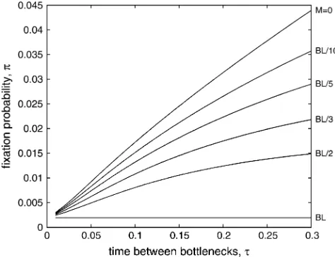
Figure 3 explores the effect of varying the time between bottlenecks, t. Similar to the case when Figure3.—Fixation probability depends on the time
be-tween bottlenecks. The fixation probability for a beneficial mutation that first occurs just after a bottleneck (at time 0) is plotted againstt, the time between bottlenecks. The wild-type population has a constant burst size,B¼100, and a con-stant burst rate,L¼1, while the death rate,M, is zero (pure burst),BL/10,BL/5,BL/3,BL/2, orBL. Beneficial mutations confer an increased burst rate, such that the mutant burst rate
lis given byL(11d). We plot results for each wild-type death rate (labels on right axis) fort-values ranging from 0.01 to 0.3. WhenM¼BL, the population size is constant; this represents the limit when the fraction of individuals who survive each bottleneck,D, is one. In all other cases, fixation probability for a mutation that occurs early during the growth phase in-creases with longer intervals between bottlenecks. We vary the time of first occurrence of the mutation in Figure 4.
Figure2.—Fixation probabilities in populations with
peri-odic bottlenecks. Here BL $ M such that the population grows between bottlenecks, which occur in these examples ev-eryt¼0.3 time units. The fixation probability for a beneficial mutation that first occurs just after a bottleneck (at time 0) is plotted against the mutant burst size or burst rate. The wild-type population has a constant burst size,B¼100 and con-stant burst rate,L¼1, while the death rate,M, is zero (pure burst model),BL/10,BL/5,BL/3,BL/2, orBL. In a, benefi-cial mutations confer an increase inB, such that the mutant burst sizebis given byB1DB. We plot results for each wild-type death rate (labels on right axis), forDBranging from 1 to 100. In all cases, as burst size increases the fixation probability approaches a plateau that is,1. In b, beneficial mutations in-stead confer an increase in mutant burst rate, such thatl¼
population bottlenecks are added to classic life-history models (Wahl and Gerrish 2001; Heffernan and
Wahl 2002), we find that longer periods of growth
between bottlenecks increase the chance that a benefi-cial mutation will survive. Once again, this effect is most pronounced when growth between bottlenecks is rapid, and bottlenecks are severe (M¼0). We note that for the parameter sets illustrated here, the bottleneck fraction D¼e(BLM)t
ranges from 1 (atM¼BL) to 1013(atM¼
0) whent¼0.3. Thus values ofton the right side of Figure 3 may not be experimentally feasible whenMis small.
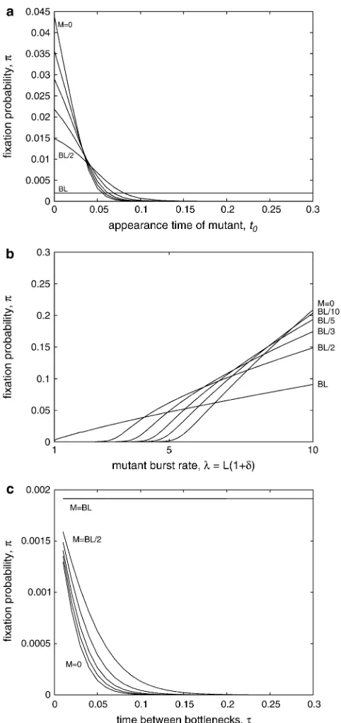
The results illustrated in Figures 2 and 3 sensitively depend on the time at which the mutation first occurs; we explore this effect in Figure 4. In Figure 4a, we find, not surprisingly, that p is much higher for mutations that occur early during the growth phase and that this effect is more pronounced when the bottlenecks are more severe. In the limit, for a constant population size (M¼BL), the time at which the mutation occurs does not affect the fixation probability.
In Figure 4b, we repeat the results shown in Figure 2b, but use a mutation that first occurs near the end of the growth phase, at t0¼0.25 when t¼0.3. We see that
whensis small, the relative influence of death between or during bottlenecks is reversed: for mutations that occur just before the bottleneck, severe bottlenecks are a more important factor than the death rate between bottlenecks. This effect is mitigated whensis very large, presumably because the burst rate is sufficiently high that a burst may occur before the bottleneck.
Finally, in Figure 4c, we repeat the results shown in Figure 3, but for a mutation that occurs near the end of the growth phase, att0¼0.85t. Here again we observe a
reversal of previous observations: for mutations that occur late in the growth phase, a long period of growth does not increase the fixation probability; rather, a less severe bottleneck increasesp. We present and discuss a summary of the key results from these figures in the following section.
DISCUSSION
The fixation probability of a beneficial mutation is sensitive both to the life history of the organism and to the means by which the mutation changes that life his-tory, which we call themechanismof the selective advan-tage. The burst–death model examined here proposes a life-history model that is mathematically tractable, but
Figure 4.—Fixation probability depends on the time at
which the mutation first appears. In a, we plot the fixation probability for a beneficial mutation that first occurs at time
t0, whent, the time between bottlenecks is 0.3. The wild-type
population has a constant burst size, B¼ 100, and constant burst rate, L ¼ 1, while the death rate, M is zero, BL/10,
BL/5,BL/3,BL/2, orBL(labels on left). Beneficial mutations confer an increased burst rate, such that the mutant burst rate
lis given byL(11d), withd¼0.1. Note that whenM¼BL, the population size is constant; in all other cases, fixation probability decreases for mutations which occur late in the growth phase. In b, we consider the case whent¼0.3 and
t0¼0.25, butlvaries. For mutations of small to moderate
ef-fect that occur near the end of the growth phase, fixation probability is increased when the background death rate is in-creased, and thus the bottleneck is less severe. In c, we repeat the results shown in Figure 3, but for a mutation that occurs near the end of the growth phase, att0¼0.85t. For mutations
may be more appropriate, for many organisms, than classic models that assume fixed generation times and no death between generations.
For populations that maintain a constant size, we find that the fixation probability,p, predicted in a burst-death model is substantially lower than that predicted in the classic case. This is because the death rate has an impor-tant effect onp, and this death rate must be quite high to maintain a constant population size when the burst size is large. Overall, we see that the classic 2s approx-imation is a very poor predictor of fixation probability when death occurs between generations.
We also note that the mechanism of the selective ad-vantage plays a crucial role in predicting p. For pop-ulations that maintain a constant size, the fixation probability is higher for mutations that increase burst rate, rather than increase burst size, for the same se-lective advantage. The fundamental insight here is that extinction is almost entirely determined by the ways in which the mutant lineage may die, be cleared, or fail to produce offspring during the first few generations of its existence. In constant-size populations, there is no death via bottlenecks, and new mutations are lost only through the death ratem, during the period before the first burst. Since the probability of dying before bursting ism/(m1l), increases inlthus have a profound effect on extinction probabilities in the burst–death model.
In contrast, in the classic model (generation times are fixed but offspring numbers are stochastic, with no death between generations), we find the reverse effect: increases in offspring number are predicted to confer a largerp, for the same value ofs, than reductions in gen-eration time (Wahland DeHaan2004). This is because,
in the classic model, mutant lineages are lost only by having zero offspring. Since increasing offspring number (the mean of the stochastic offspring distribution) re-duces the probability of having zero offspring, increas-ing burst size has a profound effect on extinction.
When population bottlenecks are imposed, the pre-dictions of the burst–death model depend on when, during the growth phase, the mutation first occurs. For mutations that occur early during growth,pis increased by reducing the death rate between bottlenecks and in-creasing the time between bottlenecks. For mutations that occur late in the growth phase,p is increased by reducing the severity of the bottleneck, which occurs when the time between bottlenecks is short. We also see thatpmay be orders of magnitude larger for mutations that occur early during the growth phase. However, since many more mutations will occur late during growth when the wild-type population is large, the ‘‘best’’ time at which to impose bottlenecks is unclear. Thus a goal for future work is to predict, using the burst–death model, the time between bottlenecks that will maximize the overall rate of adaptation (see Wahlet al. 2002).
The dichotomy between burst rate and burst size mu-tations described above for constant populations may or
may not hold, in general, once population bottlenecks are introduced. When new mutant lineages may also be lost in the bottleneck, we expect that the effect of burst size or burst rate mutations will be sensitive to the time at which the mutation first appears or to the balance be-tween death rate and bottleneck severity. Elucidating this dependence on the other model parameters, in detail, is beyond the scope of this article. We are, how-ever, able to draw some conclusions in the limiting case whensis large, even in the presence of bottlenecks. In this situation, the burst–death model predicts thatphas an upper bound, which can be much less than one, for mutations that increase burst size. In other words, once the burst size is sufficiently large relative to the wild type, the fixation probability no longer depends on burst size, but depends only on the probability of bursting before dying. In contrast, the fixation probability does ap-proach one in the burst–death model when the burst rate,l, is increased andsis very large. Recent work by Bullet al. (2006) has elucidated the dynamics of
adap-tation when changes in both burst size and lysis time are possible.
A necessary extension of our approach is to relax the assumption that the probability of reproducing is con-stant, irrespective of the age of the organism. In partic-ular, a model that is appropriate for lytic viruses when both attachment and lysis times are nonnegligible would clearly extend the experimental relevance of the work. Such a model introduces a delay term in the partial dif-ferential equation (Equation 5) and thus presents both analytical and numerical challenges.
We thank two anonymous referees whose insightful comments im-proved the manuscript. This work was supported by the Natural Sciences and Engineering Research Council of Canada and by the Ontario Ministry of Science, Technology and Industry.
LITERATURE CITED
Abedon, S. T., T. D. Herschlerand D. Stopar, 2001 Bacteriophage
latent-period evolution as a response to resource availability. Appl. Environ. Microbiol.67:4233–4241.
Allen, L. J. S., 2003 An Introduction to Stochastic Processes With Appli-cations to Biology, Ed. 1. Prentice-Hall, Upper Saddle River, NJ. Bull, J. J., M. R. Badgett, H. A. Wichman, J. P. Huelsenbeck, D. M.
Hilliset al., 1997 Exceptional convergent evolution in a virus.
Genetics147:1497–1507.
Bull, J. J., M. R. Badgettand H. A. Wichman, 2000 Big-benefit
mu-tations in a bacteriophage inhibited with heat. Mol. Biol. Evol.
17:942–950.
Bull, J. J., J. Millstein, J. Orcuttand H. A. Wichman, 2006
Evo-lutionary feedback mediated through population density, illustrated with viruses in chemostats. Am. Nat. 167: E39– E51.
Burch, C. L., and L. Chao, 1999 Evolution by small steps and
rug-ged landscapes in the RNA virusf6. Genetics151:921–927. Burch, C. L., and L. Chao, 2000 Evolvability of an RNA virus is
de-termined by its mutational neighbourhood. Nature 406:625– 628.
Fisher, R. A., 1922 On the dominance ratio. Proc. R. Soc. Edinb.50:
204–219.
Gerrish, P. J., and R. E. Lenski, 1998 The fate of competing
ben-eficial mutations in an asexual population. Genetica102/103:
Grimmett, G. R., and D. R. Stirzaker, 2001 Probability and Random Processes, Ed. 3, pp. 268–273. Oxford University Press, Oxford. Haldane, J. B. S., 1927 The mathematical theory of natural and
artificial selection. V. Selection and mutation. Proc. Camb. Philos. Soc.23:838–844.
Heffernan, J. M., and L. M. Wahl, 2002 The effects of genetic drift
in experimental evolution. Theor. Popul. Biol.62:349–356. Manrubia, S. C., C. Escarmis, E. Domingo and E. Lazaro,
2005 High mutation rates, bottlenecks, and robustness of RNA viral quasispecies. Gene347:273–282.
Sanjua´ n, R., J. M. Cuevas, A. Moyaand S. F. Elena, 2005 Epistasis
and the adaptability of an RNA virus. Genetics 170:1001– 1008.
Taylor, H. M., and S. Karlin, 1998 An Introduction to Stochastic Mod-eling, Ed. 3, pp. 355–364. Academic Press, San Diego.
Wahl, L. M., and C. S. DeHaan, 2004 Fixation probability favors increased
fecundity over reduced generation time. Genetics168:1009–1018. Wahl, L. M., and P. J. Gerrish, 2001 The probability that beneficial
mutations are lost in populations with periodic bottlenecks. Evolution55:2606–2610.
Wahl, L. M., P. J. Gerrishand I. Saika-Voivod, 2002 Evaluating the
impact of population bottlenecks in experimental evolution. Genetics162:961–971.
Wichman, H. A., M. R. Badgett, L. A. Scott, C. M. Boulianneand
J. J. Bull, 1999 Different trajectories of parallel evolution
dur-ing viral adaptation. Science285:422–424.
Wilke, C. O., 2003 Probability of fixation of an advantageous
mu-tant in a viral quasispecies. Genetics163:467–474.
Communicating editor: M. W. Feldman
APPENDIX
To derive Equation 5, from first principles, we letG(x,t) be the probability generating function for the number of individuals in the mutant lineage at time t,
Gðx;tÞ ¼p0ðtÞ1p1ðtÞx1p2ðtÞx21 . . . ¼
X‘
i¼0 piðtÞxi;
wherepi(t) is the probability that there areiindividuals in the lineage at timet. For convenience, we usepito denote pi(t) in the following. Note that
@G
@x ¼p112p2x13p3x
21 . . . ¼X
‘
i¼1
ipixi1: ðA1Þ
Now consider the possible changes toG(x,t) in a small interval of time,Dt. At timet, the lineage consists of a single individual with probabilityp1, and a burst occurs with probabilitylDt. If such an event occurs, the probability mass
must be subtracted from the coefficient ofxand added to the coefficient ofx11B. There are two individuals in the lineage at timetwith probabilityp2, and in this case a burst occurs with probability 2lDt. Using the same logic for
deaths, we derive
Gðx;t1DtÞ Gðx;tÞ ¼ ð1Þp1lDtx1ð1Þp1lDtx11b
ð2Þp2lDtx21ð2Þp2lDtx21b
.. .
ð1Þp1mDtx1ð1Þp1mDt
ð2Þp2mDtx21ð2Þp2mDtx
.. .
In the limit asDt/0, we therefore have
@G
@t ¼ ðl1mÞ
X‘
i¼1
ipixi1lX
‘
i¼1
ipixi1b1mX
‘
i¼1 ipixi1
¼ ðl1mÞxX
‘
i¼1
ipixi11lxb11
X‘
i¼1
ipixi11m
X‘
i¼1 ipixi1:
Using Equation A1, we have thus derived Equation 5:
@G
@t ¼ ðlx
b11 ðl1mÞ
x1mÞ@G @x:
This equation is a Lagrange-type partial differential equation, which takes the form
Pðx;t;GÞ@G
@x1Qðx;t;GÞ
@G
This can be solved using the auxiliary equation
dx P ¼
dt Q ¼
dG R;
which in our case yields the following two equations:
dx P ¼
dt
Q ðA2Þ
Rdt¼QdG: ðA3Þ
If we are able to solve for two independent solutions of the auxiliary equation,
f1ðx;t;GÞ ¼c1; f2ðx;t;GÞ ¼c2;
wherec1andc2are constants, then the general solution of the Lagrange-type PDE can be given as
Fðf1ðx;t;GÞ; f2ðx;t;GÞÞ ¼0; whereFis an arbitrary analytical function and can be solved explicitly forG.
From Equation A3, we find thatdG¼0, orG(x,t)¼c1, and so we takef1to be simplyG. Integrating Equation A2, we
find
ð dt¼
ð
1
lxb11 ðl1mÞx1mdx t1c2¼
ð 1
ðx1Þðlxb1lxb11 . . . 1lxmÞdx
t1c2¼ 1
blm logðx1Þ Xb
i¼1
logðxxiÞLi
! :
The previous step is obtained by partial fraction expansion, wherexiare thebroots of the polynomiallxb1l
xb11
. . .1lxm, and theLiare given by
Li¼ Pb
j¼1jx
bj i
Pb
k¼1kxik1
:
In general, these roots cannot be found analytically, especially asbincreases, but can be easily found numerically. We thus take the arbitrary analytical functionFðGðx;tÞ;ðblmÞt1logðx1Þ Pb
i¼1logðxxiÞLiÞ ¼0:We rearrange
this to find thatG(x,t) is given by some analytical functionH(w), where
w ¼e
ðblmÞtðx1Þ
Qð
xxiÞLi : ðA4Þ
Our solution must satisfy the boundary conditionG(x, 0)¼x, so we sett¼0 in Equation A4 and solve forx. The solution to this procedure yieldsG(x,t), which must be on the interval½0, 1. In simple cases, such as whereb¼1, this can be solved analytically. In the general case, we find thatG(x,t) is given by the value ofyon½0, 1that is a root of the equation
eðblmÞtðx1Þ Q
ðxxiÞLi
Y
i
ðyxiÞLiy11¼0: ðA5Þ