Model based recognition of 3-D surfaces using curvature parameterization

(1)

Model Based Recognition Of

3-D

Surfaces

Using

Curvature Parameterization

by

s.

J. Garnier

G. L.

Bilbro W. E. Snyder

Center for Communication.s and Signal Processing Department of Electrical and Computer Engineering

North Carolina State University

CCSP-TR-89/6

(2)

A new approach to rigid object recognition in range imagery is presented. This approach is based on a special re-parameterization of a smooth surface that is independent of rotation, translation, or surface parameterization. An observed surface point always transforms to identical coordinates in the special parameter system. This property allows a correspondence between points on two surfaces and permits comparison of the surfaces by correlation techniques.

(3)

Model Based Recognition Of 3-D Surfaces Using Curvature Parameterization 1

1 Introduction

This paper investigates a recently developed [6] approach to rigid object

recog-nition in range imagery, and is based on a special re-parameterization of a smooth

surface that does not depend on the conditions of rotation, translation, or

param-eterization of the surface.

The special re-parameterization utilizes a differential geometric formalism, and

is based on determining the principal curvatures of the points of interest, and then

using the principal curvatures as axes of the parameterized coordinate space.

For a continuous surface, an arbitrary point on the surface will always

trans-form to numerically identical coordinates in the special parameter system,

inde-pendent of observation pose. This amounts to a continuous correspondence

be-tween points on two surfaces and permits the matching of surfaces by correlation

techniques.

In section 2, a general derivation for the parameterization is given, utilizing

a continuous formulation. In section 3, the concept is formulated in a discrete

manner amenable to implementation on a digital computer. This formulation is

stated as an algorithm in section 4. The technique is tested on range images in

section 5, and shown to be an effective visible-invariant means for recognizing

(4)

2 Problem Formulation

We consider a surface in 3-space as a mapping, X, from a set of points in a

parameterizing plane U ~ R2

, to a set of points in 3-space

(1)

(2)

In this paper, we assume X is a three times differentiable manifold. That is,

~Y is specified by three parametric equations

x(u) = [

:~:::~

] where u = (u,v). z(u,v)

The actual surface X(U) is invariant to observation viewpoint, but the details of the parameterization are not unique. The same surface may be represented by Al(V) where AI :V - 4 ~3, and M is some triple of functions different from those of X defined on some different domain set V. Or, the surface M(V) may be a rotated or translated duplicate of X(U). Or it may be another surface entirely. If we denote the image or observed surjace as ~Y(U) and the model surface as

AI(v

Y

),

the question of interest is whether X(U) is congruent to 1\J(V). That is to say, does there exist a rigid body motion, R, such that ..IY(U)

==

RM(V)?

We will employ the surface curvature to answer this question. We are particu-larly interested in curvature since it is viewpoint-invariant. That is, the curvature of a surface at a point is a property of the surface, and not a property of how the surface is observed. We will make extensive use of this property.

(5)

range camera [2] , we determine the principal curvatures through the use of the

first and second fundamental forms [14, pp.107-112] [19, pp.67-93] of differential

geometry. The first fundamental form is the determinant of G where

Br 8r 8r 8r

Gu v

=

8~ 8~ Bu • av

(3)

8r Br 8r Br Bv · Bu Bv •

av

and where the parametric surface r

=

r(u,v)

=

[!(u,v),g(u,v),h(u,v)]T.

G (also known as "the metric of the surface") may also be written in terms of the

[x,

y,

z]T

Cartesian coordinate vector where

z

==

z(x,

y),

Gx y

==

8zBz

8:r

By

8z 8z

8:rBy

(4)

The second fundamental form is the determinant of D where

82r ₈2r

n· - - n· - _.-Du v

==

8u2 _8u8v

(5)

82r ₈2r

n · -_8v8u n · -_8v2

and where n is the surface normal at the point of interest. Again we may write D

in terms of the

[x,

y,

z]T

Cartesian coordinate vector,

82z ₈2z

1 8;;2 8~8y

Dx y = -

(6)

s:

82z ₈2z 8:r8y 8y2

where 5, the square root of the determinant of the first fundamental matrix is.

,

the differential surface area

[25,

pp.437-441] at the point of interest:

(6)

We determine the principal curvatures, k₁ and k2 , by solving the quadratic

equation [14, pp.107-112]

det (D - kG)

==

o.

(8)

The solutions, k

==

k1 and k

==

k2 are the minimum and maximum normal

curva-tures at the point of interest. For convenience, we introduce the notation

k(x,y,z)

to represent the process of solving Equation 8 at a particular (~,y,z) on the sur-face. We refer to the mapping from the measurement parameterization to principal curvat ures as the curvature map

(9)

We will further restrict our attention to those surfaces (or segments of surfaces) which satisfy an additional property:

Consider a domain U of the imaged surface, on which the curvature map has a nonsingular Jacobian everywhere

[

8(

»;

k2 ) ]

detJ

==

det ---

==

det 8(u,v)

fu fu

au 8v

(10)

We shall call any region on which J is never singular, and where the region is the

image of a rectangle by a map which is one-to-one, a regular segment. On a regular

segment, K[ has a local inverse everywhere. [28]

Postulate: On a regular segment, the curvature map has a global inverse.

(7)

anticipation-Model Based Recognition Of 3-D Surfaces Using Curvature Parameterization 5

We have shown [6] this postulate to be true on the additional condition that the regular segment is part of a quadric surface. We believe that the quadric condition is unnecessary but we have not been able to prove our conjecture. The conjecture simplifies the theory and we will assume it to be true. Even if it is not true, the theory could be modified by using the notion of multiple valued functions borrowed

[22]

from the study of complex variables.

If K[ is invertible, then the composite function JY

0

K

1-

1 :

K1(U)

~ X(U) is

a single-valued visible-invariant parameterization of the segment, that is, for each pair of principal curvatures, a unique point on the surface is determined. A similar map can be constructed on any model segment M

0

KA{-1 : KM(V) ~ 1Vf(V).

Thus, since this type of composite map takes a pair of principal curvatures to a Cartesian triple on the surface, the entire surface is exactly represented and can be accessed by curvature pairs. As an immediate result of the curvature mapping, we have:

Corollary: If regular surfaces tJl1 and ~2 have identical curvature maps, then fill is a similarity transform of <1'2 and vice-versa.

Thus, recognition of a regular surface becomes a simple comparison of curvature maps. We are not limited to regular surfaces, however, as we will see in section 3, by taking account of the area subtended by a particular curvature map, we can distinguish even umbilic surfaces such as spheres.

(8)

curvature plane

by

dA

==

PI(k)dk2 •

(11)

pr(k)

is determined from

_{G r,}

the first fundamental form of the imaged surface by

Pr(k)

=

J(detG r) where

G_r

=

(J-l)T

GroJ-1

(12)

(13)

and the Jacobian is as defined in Equation 10. The metric G1 is positive definite

[28] in this parameterization just as is the metric in the original parameterization,

G1o , from which it is derived.

[28]

Here G10 is simply the metric in the original

(camera frame) parameterization, put forth by Equation 4.

Definition

(1):

An imaged segment is said to be congruentwith a model segment

if and only if the curvature image of the former is contained within the curvature

image of the lat ter, that is,

2. VkE

K1(U), pr(k)

==

PM(k).

From 2) it follows that,

3. _{f fkEK J}Pr(k)dk = f fkEKJPM(k)dk ·

We refer to condition 1) above as the domain test. Simply put, no point on

the imaged surface may have a principal curvature pair which is not in the model

(9)

two segments must be identical whenever the imaged surface is observed. Note

that since this comparison is only over the visible portions of the imaged surface,

occlusions are automatically handled. Similarly, condition 3) requires that the

total area subtended by the two segments be the same, again, considering only

visible area. To see that condition 3) represents the area, consider the different

parameterizations based upon, say,

(u, v)

and (z,y) of the same surface, ~, and let

tP_{u v} and cI>~ybe the domain of the surface in the

(u, v)

and (z,y) pararneterizations,

respecti vely.

(14)

(15)

(16)

Thus, if the imaged surface consists of exactly one regular segment, the

curva-ture parameterization provides a transformation which will exactly match (in the

absence of noise) the transformed model segment.

Note that in this work, we use a mapping of the entire surface into

(10)

3 Implementation

3.1 Effects of Sampling

In order to apply the strategy of Section 2 to realistic problems, we must first

consider the discrete nature of the data. Let _{M s} be the finite set of points resulting

from a sampling of the model surface AI{. Let I

=

R1Yf represent the (unknown) rigid body motion applied to M to result in the observation I, and similarly, let

Is

be the sampled version of

I.

Due to the sampling it is a virtual certainty that

there do not exist any two points XI E Is and XM E !lIs which satisfy exactly

XI

==

Rx},;/. Due to the sampling of the segments, we simply are not looking at

the same point on both the imaged and modeled surfaces.

Sampling causes no significant problems with the domain test. The sampled

representation is in error by, at most, the displacement of one pixel, and curvature

changes very little between adjacent pixels (except near a singularity, and we avoid

such points). The range test is violated by sampled data, but for the most part,

such violations nearly cancel out. When the violations do not cancel out, they are

dealt with robustly by the recognition algorithm discussed in Section 4.

We define the curvature hisioqram of the image as a douhly-indexed array

(We use notation analogous to that of Section 2, to represent analogous concepts,

(11)

confusion). We calculate SI by

Sl(k1, k2 ) =

L

pl(k(x,y,z)) where z

=

z(x,y) · ~,YEI

(18)

That is, over the surface, we sum the area subtended by all pixels in the range

image whose principal curvatures fall within the span defined by k1

±

~ ~k, k2

±

~ ~k.

Theorem (1): The volume of the curvature histogram is equal to the surface

area of the imaged segment.

This follows directly from Equations 14, 15 and 16. It is only approximately true

for sampled data, however it illustrates the strength of the method. Since the

curvature histogram is visible-invariant, and the computation of its volume is an

integral process, we have a method which is relatively robust against noise.

Definition

(2):

Let x

=

(Xl,X2) and y

=

(Yl,Y2) be two vectors in the plane ~2.

A vector z

=

(Z1,

Z2)

is said to be between x and y if and only if Xl

<

Zl

<

Y1 and

surface. Let k, and k, be the curvature mappings of a and b. Now, suppose k,

is between k, and kb • We ask the question, can S(kc )

==

O? That is, can there be

curvatures in this range which correspond to no points on the surface? Since the

(12)

think of the problem as a continuous mapping. IIowever, since both the surface and the curvature space are sampled, we should more properly ask, can holes ezisi in the curvature histogram

r

The answer is certainly yes. We could force this to happen in a trivial way by simply making ~k very small, thus producing a curvature map of fine granularity. Since each sampled point on the surface contributes to exactly one bin in 51, by sampling SI more finely, we guarantee some empty cells. Clearly, the details of the conditions under which these holes appear depend upon the sampling rate used in Cartesian space, the sampling rate in curvature space, and the rates at which the surface bends. Certainly, if the surface can undergo an abrupt change in curvature between two pixels, then with respect to a discrete curvature space mapping, there will exist at least one curvature histogram cell between the two pixels curvature histogram cells which receives no contribution. We quantify this notion with a one-dimensional argument. Let the image consist of one cycle of the function y

==

sin{ e ), and let this function be uniformly sampled by N samples spaced 6 units apart, thus 6

==

iJ.

We will now derive a relationship between N,

h

_,

and allowable values ofD&k. Given the vector r

=

[x,

y,

zf

where

r = [x,sin(x),OjT ,

r

=

[l,cos(x),OjT ,

r

=

[0, - sin(x),OjT ,

(19)

(20)

(13)

Model Based Recognition Of 3- D Surfaces Using Curvature Parameterization 11 the curvature, K, ofr is [28]

sin(

x)

3 •

(1

+

cos2

_{(x)) i}

(22)

The rate of change of curvature with respect to x is then k(x)

=

2cos(x)[1

+

sin2~x)]

(1

+

cos2₍_{X ) )}

2

and the curvature extrema occur when

(23)

By solving Equation 24, we determine the location of the maximum rate of change of curvat ure to occur at (}kmQ:I:

==

64.285 degrees. If dropouts are to occur, they

will occur in those areas of the function where K changes most rapidly. One such

point is 8k m a :I:. Moving one pixel away, we have

~

I

sin(lhmaa:

+

.5) -

sin(O;maa:)

I

==

(26)

(1

+

cos2

_(8kmQ:I:))i

==

I

sin(Okmaa:)cos(.5)

+

sin(.5) cos(

Ok~aa:)

- sin(Okmaa:)

~

(27)

(1+cos2

_(8kmQ:I:))i

6 cos(8k m a

:r )

2.1

~ (l+~o~2{8k-m-aa:))~

N (28)

(14)

4 Algorithm

In this section, we discuss the development of the model based curvature space

histogram library, and the recognition algorithm which uses this library.

4.1 Histogram Library Generation

1. For all model range images, Zm(x,

y)

where m

=

1, ... ,M, compute k_{1m(x ,}y), k2m( x ,y), and Pm(x,y).

2. For model range image Zm, determine maxkIm Similarly determine max_k2m.

3. Find the global maximum curvature maxk

==

maXm= l ,...,M(maxkIm'maxk_{2 m )}

4. Using maxk, linearly partition the principal curvature space into NxN

par-titions, which span a range of (2n

+

l)~k, from - maxk to

+

maxk. (Note

the redefinition of N, as distinguished from that used in Section 3.) We

specified N as a positive odd integer, N

==

2n

+

1, in order to force all

pla-nar surfaces to map exactly onto an origin-centered partition, all spherical

surfaces to map exactly onto partitions on the k1 == k2 line, and all minimal

surfaces to map exactly onto partitions on the k1

==

-k2 line.

(15)

In solving Equation 8 for k₁ and k2 , we arbitrarily choose the sign of the square root so that k₁

2:

k2 , and choose k1 and k2 to be the vertical and horizontal axes, respectively. This assignment maps all surfaces onto or above the 45 degree line.

If this line, originally defined by k1

=

k2 (the line of umbilic surfaces), is rotated

into the horizontal axis, then the line k1

==

-k2 (the line of minimal surfaces) is

also rotated into the vertical axis. The new horizontal "urn axis is proportional to

mean curvature, whereas the new vertical axis represents a difference curvature.

This new representation requires roughly half the storage of the original k1 ,k2

representation, since all points below the 45 degree line are of zero value. A range

image view of the exterior of an ellipsoid transforms to the second quadrant of this

new sum-difference curvature plane, and an interior view of the same object would

transform to the first quadrant, as a mirror reflection about the vertical axis.

4.2 Recognition

Surfaces are recognized USIng a rrurumum error classifier, which is based on

maximum likelihood probability estimation. The maximum likelihood estimator

we utilize compares the curvature-space histograms of the observation with the

histograms of the models. Therefore, this comparison provides a visible-invariant

method for recognition.

We wish to find the model

Zm

which maximizes the conditional probability

(16)

we define two sources of such corruption:

• accretion error

curvature value, more area has occurred in the image than in the model. The larger

the accreted area, the lower the probability that the observed surface belongs to

the model .

• occlusion error

this implies that some part of the observed surface is occluded, either by the surface itself, or by some other surface. The larger the occluded surface, the lower

the probability that the observed surface belongs to the model.

4.2.1 Likelihood of Accretion

Accretion error occurs when a binin the image curvature histogram violates either

the range test or the domain test; that is, the bin's surface area is greater than

the models surface area. We cllaractcrize this error in the following manner: Using Bayes rule, given an image

I,

the probability of accretion of a particular

(17)

We ignore the constant denominator and define the likelihood of accretion of a

particular model to be

(30)

Considering only the conditional probability, and assuming independence,

PA(IIZm)

==

PA(~lIZm)PA(~2IZm)···

=

II

PA(~iIZm)Wi (31)

+iE+

where ~ is the set of curvature bins which violate the range or domain tests. From

this we define the probability of accretion within one bin,

(32)

where NSm is the number of non-zero curvature bins in SZm.. Finally, we choose a

form for PA(tI>ilkj E SZm.). We choose a zero mean, unit variance model,

(33)

where _dij is the Euclidean distance from bin j to bin i in the curvature histogram.

In Equation 31, ltl'i is a weight which reflects our intuitive understanding that

the magnitude of the range test violation should effect the probability of

occur-renee:

(34)

The probability of accretion within one bin should reflect the relative size of ea.ch

(18)

has a greater probability of contributing accretion area to an image bin than does

a smaller model bin. We modify Equation 32 in order to weight the probability of

occurrence with respect to the relative sizes olfeach donor bin:

4.2.2 Likelihood of Occlusion

The probability of occlusion of a particular model is determined using Bayes rule,

and is similar to that expressed in Equation 29:

Again ignoring the constant denominator, we define the likelihood of occlusion of

a particular model to be

Assuming independence of the individual occluded curvature bins, we obtain

Po(IIZm)

==

II

Po

(0

iIZm) 0iE0

(37)

(38)

where 0 is the set of curvature bins which exhibit occlusion. We define the

prob-ability of occlusion within one bin,

(39)

where a is an appropriate normalization. Here we assume that for each curvature

(19)

error applied to the corresponding pixels in the model is Gaussian. SinceSZm(ki )

-SI(k_{i )} is strictly positive for all

E>i

E

e

(by definition of occlusion error), and we will momentarily take the logarithm, we omit the square and define a

non-normalized likelihood:

Hence, by reflecting this likelihood into Eqllation 38, we have

Lo(IIZm)

==

II

exp {-[Szm(ki ) - SI(ki ) ] } • 0iE0

4.2.3 Minimum Error Classification

(40)

(41)

Finally, we define total likelihood as the product of the independent probabilities

and likelihoods due to occlusion and accretion:

(42)

We derive a minimum error classifier from the maximum likelihood estimator

by taking the negative of the natural logarithm of Equation 42. We obtain the

total error:

Error(m) = Erroro(m)

+

ErrorA(m) . (43) The model with the minimum error is selected as the most likely match for the

Image.

We now develop the accretion error by taking the negative logarithm of the

(20)

exhibit accretion with respect to each model is N~m.

ErrorA(m) = -log{PA(Zm)}

+

N~mlog{NSmlTy!2;

L

SZm(k_j

)}+

(44) kjESzm

+

L

[Sr(ki ) - SZm(ki ) ] -

L

log [

L

exp

{_!

(d

ii

)2}Szm(k

_j) ]

+iE+ +iE~ kjESz", 2 o

Similarly, we develop the occlusion error by taking the negative logarithm of

the occlusion likelihood:

Erroro(m)

=

-log{PO(Zm)}

+

L

[Szm(k_{i ) -} Sr(k_{i ) ] •} (45) E>iE0

In Section 5, we assume the a priori probabilities, PA(Zm) and PO(Zm),to be

identical for all models, and therefore ignore this term while calculating the total

error.

4.3 Recognition Algor-ithm

1. The curvature histogram of the range image to be recognized is computed

in a manner similar to tile method described in Section 4.1.

2. For each model, m, the total error is computed as shown in Equation 43.

3. The image is recognized as belonging to the model wit.h the minimum error.

5 Performance

The recognition algorithm discussed in Section4 was tested using both synthetic

(21)

deter-Model Based Recognition Of 3-D Surfaces Using Curvature Parameterization 19

mine the sensitivity of the algorithm to noise, data with well-controlled statistical

properties was required. Therefore, synthetic images were generated [20] which

represent rotated and translated octant and sub-octant patches from one of the ten

ellipsoid octant models (specifically ellipsoid model 5). These ten ellipsoid models

vary in only one of their major axes. We note from Tables 1 and 2 that models 4,

6 and 7 are very similar to model 5 (indistinguishable to a human observer), and

the algorithm matching corrupted images extracted from model 5 can be expected

to fail most often by classifying the unknown as case 4, 6 or 7. Indeed, the

experi-ments confirm this expectation. The synthetic image patches were corrupted with

white Gaussian noise. After preprocessing, the resulting range image was matched

using the total error measure defined by Equation 43.

To build the model histogram library, a range image synthesis program [20]

was used to generate three quarter-cylinder models, ten different ellipsoid-octant

models, and cone, hyperboloid, and sphere models. The model-based curvature

histogram library is developed using the algorithm described in Section 4. Even

though these surfaces are used in our experiments, it should be emphasized that

the objective of this work is not to recognize only quadric surfaces. (See Faugeras

[13] for an excellent approach to quadric surface recognition.) Ellipsoids arid other

quadric surfaces were used in these experiments for ease of synthesis a.nd analytic

tractability. However, there is nothing in the algorithm that requires analytic

(22)

Table 1: The Quadric Models

Semi -majo~Axi~--tm-ith~--(pixei-;fiit-Ieng

t~---Models a b c

ellipsoid model 1 66.6667 100 200

ellipsoid model 2 66.6667 100 141.421

ellipsoid model 3 66.6667 100 115.47

~liipsoid~od~i4

--66:66670-

100

_..

-100

eilip~~id

mo-del

5 66.6-667

-

_._-~--100 89.4427

ellipsoid model 6 66.6667 100 81.6497

ellipsoid model 7 66.6667 100 75.5929

ellipsoid model 8 66.6667 100 70.7107

ellipsoid model 9 66.6667 100 66.6667

ellipsoid model 10 66.6667 100 63.2456 t~~~cat~J-~one2model

11

--_.-._----.50 to 100- 50 to 100--- - - - - -hY·p-erb-oloi~:f3m~-dei-12-n_.--_.- -- --- ----. _.._.-- .---.

-100 89.4427

-sphere model 13 100 100 100

cylinder model 1 16.1937 16.1937

-cylinder model 2 14.7479 14.7479

-cylinder model 3 12.6491 12.6491

-The sensitivity of the algorithm was tested with respect to cardinality and to

noise. By cardinality, we mean the number of pixels in the observed portion of

the image surface. Cardinality is distinguished from area since a single pixel can

subtend a vast range of possible areas, depending on its orientation with respect to

the viewpoint. In the following sections, the term noise will refer to the variance

of white Gaussian noise added to the image. Tests were run with preprocessing

described in Section 5.1.

2See Table 2for additional clarification.

(23)

Model Based Recognition Of 3· D Surfaces Using Curvature Parameterization

21

Table 2: Coefficients of the Quadric Models r---A~-2

+-B

y

2 -

+--0

~-2

-~-'b2---Models

A

B

C

D

ellipsoid model

1

9 4 1

200

ellipsoid model

2

9 4

2

200

ellipsoid model 3 9 4 3

200

~~iiips;;rJ mod~l

4-

-_._- - - -- - - - f _ . ._

-9 4 4

200

-.-- - -

-

-200--~ilip-;~id mod~i-5 9 4 5

ellipsoid model 6 9 4

6

200

ellipsoid model

7

9 4 7

200

ellipsoid model

10

9 4

10

200

--t~~ncated co~~4model

11

4

-1

4

0

-·hyp;ib~i~fd5m~d~f-l~--9

--4

5

200

sphere model 13 1

1

100

cylinder model 1 0 1 1 16.1937 cylinder model

2

0

1

14.7479

cylinder model 3 0 1 1

12.6491

5.1 Preprocessing

Prior to mapping a noisy surface into principal curvature space, we must

pre-process the noisy range image in order to extract meaningful first and second order

derivatives from the underlying surface of the data. This is accomplished in this

paper by using various combinations of three techniques:

1. Iterative Gaussian smoothing, or

2. Mean Field restoration, or

4The cone is truncated such that 50 ::;

J

Z 2

+

z2 ::; 100.

5The hyperboloid suboctant patch is constrained by z > 0, Y> 0, and z >

o.

Then, in order, it is pitched 35.26 degrees about the y-axis, yawed 45 degrees about the x-axis, translated 10, 70, and 60units in the x, y, and z directions, respectively, and finally constrained within a 256by 256

(24)

3. MSE fitting of the data to some particular surface type, such as a quadric [13].

Iterative Gaussian smoothing [10] uses the smallest smoothing kernel possible

[26],

thus preserving resolution, and produces floating point output. Iterating the

pro-cess results in the equivalent of a large kernel.

In a separate work [5]

[16] ,

the authors of this paper set up a restoration

problem which required that

1. the restored data should be similar (in the MSE sense) to the data, and

2. the restored data should be locally smooth.

This problem formulation resulted in a minimization problem which was solved

using Mean Field Annealing [7]

[16]

(MFA). The algorithm performed

spectacu-larly well on range images of polyhedra, removing noise while preserving edges.

When applied to quadric surfaces, the algorithm produced excellent, although not

perfect, restorations. This same software was used in some experiments described

in this section.

In Figures 1 through 4, we show the error generated when comparing rotated,

translated, noisy subimages of ellipsoid model 5 with each of the ten ellipsoids,

truncated cone, hyperboloid, and sphere models. In each graph, the error resulting

from comparing the model 5 subimages with model i is indicated by the numberi

immediately adjacent to the corresponding error curve. Thus, whenever the error

(25)

occurs. In Figures 1 through 4, note the relatively large separation between the

recognition error measurements of model 5 and models 11, 12, and 13 (truncated

cone, hyperboloid, and sphere, respectively).

5.2 Results: Preprocessing Using Gaussian Smoothing

Noisy synthetic quadric data was processed with iterative Gaussian smoothing.

Curvatures were determined from the smoothed surface.

5.2.1 Sensitivity to Cardinality

Figure 1 illustrates the recognition results after smoothing by showing the error

measure versus cardinality for a fixed Gaussian noise standard deviation, a.;

==

0.30. Figure 1 clearly shows how important it is to have relatively large image

segments to work with, when trying to classify very similar objects. Error for

the correct class drops, while erroneous matches have errors which grow relatively

rapidly (note log scale) with cardinality. The error "spikes" which occur at lower

cardinalities are due to the relative placement of a small image with respect to

ellipsoid model 5. Extracting a small image from a highly identifiable portion of

a model will cause the algorithm to produce relatively large errors for models not

possessing those image curvatures. Conversely, extracting a small image from an

area which is not uniquely identifiable will cause similar error values for several

models. Lower cardinality images were extracted from different regions of model 5.

(26)

Figure 1: Error vs. Cardinality, Un = 0.30

tn

o

~r----'---,r---'---r---_

___ ---·12

L

a

L L

tl)

11

:t-O

-t

0.00

0.50 c ar-d

i

na

l

i

ty

1.00 (x

1

O~)

5.2.2 Sensitivity to Noise

Figure2 illustrates the recognition results after smoothing by showing the error

measure versus the Gaussian noise standard deviation for a fixed cardinality of

8530. Here, the error associated with grossly incorrect matches actually declines

with increasing noise. This rather anomalous result is explained by the fact that

an increase in the standard deviation of noise was dealt with by a linear increase

(27)

Figure 2: Error vs. O"n, Cardinality

=

8530

If')

~..---...--..,.--~-...,.--r---r---r--.--...---'

12

---11

L

o~

L ...

L

~

I I5

I

0.80 0.20

(T1

0L.---..l._----L_-L-_...L..-_L--..l.----'----L.--...I.-~

-0.00

o.

~o 0.60 1.00

sIgma

5.3 Results: Preprocessing Using Quadric Fitting

Noisy synthetic quadric data was

MSE

fitted with a quadric surface. Curvatures were determined from the fitted surface.

5.3.1 Sensitivity to Cardinality

Figure 3 illustrates the recognition results after quadric surface fitting by

show-ing the error measure versus cardinality for a fixed Gaussian noise standard

de-viation of 0.30. Again, we note that the decline in error rate for larger images

is dramatic, and that error "spikes" (explained in Section 5.2.1) occur for lower

(28)

5.3.2 Sensitivity to Noise

Figure 4 illustrates the recognition results after quadric surface fitting by

show-ing the error measure versus the Gaussian noise standard deviation for a fixed

cardinality of 8530.

5.4 Tests 'With Industrial Tmages

To further test the algorithm, two images of cylinders were obtained, using the

GE [1] range camera. In addition to the high levels of noise found in present laser

triangulation range scanners, these images (Figure 5) exhibited a large number of

dropouts (points where the scanner simply returned no data), and some geometric

distortion. Dropouts apparently occurred often in this data because the surfaces

were metallic and somewhat specular.

In order to correct for dropouts in these cylinder images, prior to submittal

to the recognition algorithm, these images were first preprocessed by a median

filter. Noise was removed from the median filter output by the MFA restoration

algorithm mentioned in Section 5.1. The MFA output was then operated upon by

quadric surface fitting. After fitting, the result.ing range images were compared

to cylindrical models using the total error measure, defined by Equation 43. The cylinder images have cardinalities of 1595 and 1424 pixels. Gaussian smoothing

(29)

Model Based Recognition Of 3- D Surfaces Using Curvature Parameterization 27

Figure 3: Error VB. Cardinality, Un = 0.30

If) l,....'l

--4.---...---...----,---,.---r---,---,

_ - - - 12

--,---L_r

0 0 L -4

L (l)

0.50 1.00 1.50

card1na

11

ty (xlO't)

Figure 4: Error V5. Un, Cardinality

=

8530

J

1 I

I

t.n

o

--4r---....---r---~--__r_---_--_

__________________________________ - - - 12

-I I I

2.00

sigma

«in»

I

i.en

(30)

compared to all the models are presented in Table 3.6

M

Table 3· C 1·yIn erd Recognl Ion rror easurements total error total error Models for cylinder 1 for cylinder 2 ellipsoid 1 _1.70e+38 _1.70e+38 ellipsoid 2 _1.70e+38 _1.70e+38 ellipsoid 3 1.70e+38 1.70e+38 ellipsoid 4 1.70e+38 1.70e+38 ellipsoid 5 1.70e+38 1.70e+38 ellipsoid 6 1.70e+38 1.70e+38 ellipsoid 7 1.70e+38 1.70e+38 ellipsoid 8 1.70e+38 1.70e+38 ellipsoid 9 1.70e+38 1.70e+38 ellipsoid 10 1.70e+38 1.70e+38 truncated cone 11 1.70e+38 1.70e+38 hyperboloid 12 1.70e+38 1.70e+38

sphere 13 1.70e+38 1.70e+38

cylinder 1 2.06e+03 2.0ge+03 cylinder 2 2.00e+03 1.5ge+03 cylinder 3 1.70e+38 1.64e+03

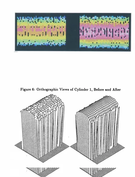
--In Table 3, we note that while the algorithm clearly distinguishes between the

cylinders and the other surfaces,it confuses the range image of cylinder 1 with the model of cylinder 2. To see the reason for this, observe Figure 6 which presents

orthographic views of cylinder 1, before and after preprocessing. It is clear from

these images that, due to geometric distortion in the camera, the image is simply

not cylindrical.

(31)

Model Based Recognition Of 3-0 Surfaces Using Curvature Parameterization 29

Figure 5: Dropouts in Range Data

(32)

6 Conclusion

In this paper, we have presented a viewpoint-invariant method for recognition

of curved surfaces in range images. Although we have given considerable

atten-tion to regular surfaces, the method is by no means limited to such surfaces. A

sphere, for example, will produce a sharp peak somewhere along the line k₁ = k₂

-Furthermore, two spheres may be distinguished by the location of the peak along

that line, which is determined by the radius.

The method is tolerant of partial occlusion. Such an occlusion simply reduces

the height of some bins in the histogram. This fact contributes significantly to

the power of the result: the method does not depend on an accurate

segmenta-tion. Segmentation errors which cause region fragmentation [30] or which, due to

boundary effects, reduce region size, are automatically accommodated. The

con-struction of the curvature histogram is fundamentally an integral process, making

the method somewhat robust under such errors. Region blending [3]

[17] ,

the other type of common segmentation error, will cause erroneous results. However,

most segmentation algorithms may be tuned to favor either region fragmentation

or region blending. To use this algorithm, one should tune the segmenter to be prone to fragmentation (also referred to as over seqmerdaiion.[. The curvature

histogram may then be used to not only recognize the region, but will also serve

(33)

strategies [11] , or as mappings onto a parameter space such as the Gauss sphere

[18, 365-391] .

The principal criticism which may be leveled against this technique has nothing

to do with the technique at all: it is the fact that given a noise-corrupted surface,

the input (curvature of the underlying surface) is difficult to accurately estimate.

The purpose of this paper is not to address how to calculate curvature. In this

sense, we philosophically follow the lead of researchers in optical flow [21] [24]

[27] who assume that a disparity map [27] or motion field [21] [24] is available,

and show that a wide variety of powerful conclusions may be drawn. Accurate

estimation of disparity maps and motion fields is often exceedingly difficult since

it requires solution of the correspondence problem.

We are not discouraged by the difficulty inherent in curvature calculation. In

this paper we used three different preprocessing techniques to smooth the images

and then computed curvatures in a rather straightforward way. We had reasonable

success in distinguishing between surfaces which were very similar (recall Table 1).

Other researchers in our own laboratory, as well as others [9] [23] , are actively

pursuing improved methods of curvature estimation. Guckin [15] has shown that

fitting a paraboloid can provide invariant local estimates of curvature, provided

that fit is performed in the locally tangent frame. (Of course, the tangent frame

is also unknown, requiring an iterative algorithm). Guckin's work is similar to

(34)

that Guckin does not explicitly model discontinuities. Guckin finds this adequate

for invariant detection of step and roof edges using a single constant threshold.

Other researchers have posed restoration problems which remove noise while

pre-serving edges, using assumptions that the surface is locally constant

[16] [29]

[8]

or locally planar [4] [8] , with excellent results. Although we have not yet had

the opportunity to perform the experiment, it seems straightforward to formulate

such a restoration which assumes the surface is locally homogeneous in curvature.

It is likely that such a restoration technique would further reduce the frequency

of image misclassification,

Finally, if one is fortunate enough to be dealing with surfaces of a known

analytic form (e.g. quadrics) [13] , truly superior curvature estimates may be

produced by first fitting the entire surface with a single function.

Thus we have a 3-D surface recognition method which is robust and

viewpoint-invariant, provided relatively good estimates of curvature may be determined, and

(35)

References

[1]

Vivek Badami, Nelson R. Corby, Nancy H. Irwin, and Ken Overton. Using range data for inspecting printed wiring boards. In Proceedinqs of Interna-tional Conference on Robotics and A utomation, IEEE, Philadelphia, April 1988.

[2] P.J. Besl. Active, optical range imaging sensors. Machine Vi3ion and Appli-cations, 1(2), 1988.

[3] G. L. Bilbro, Carla D. Savage, and W. E. Snyder. Identifying Region Adja-cency Graphs Degraded by Feature Blending. Technical Report CCSP- WP-85/12, Available from the Center for Communications and Signal Processing, North Carolina State University - Raleigh, June 1985.

[4] G. L. Bilbro and W. E. Snyder. Range Image Restoration Using Mean Field Annealing. Technical Report NETR 88-19, Available from the Center for Communications and Signal Processing, North Carolina State University, 1988.

[5] G. L. Bilbro and W. E. Snyder. Range image restoration using mean field annealing. In Advances in Neural Network Information Processing Systems, Morgan-Kauffman, San Matao, CA, 1989.

[6] G. L. Bilbro, W. E. Snyder, and J. E. Franke. A Linear Time Theory for Recognizing Surfaces in :J-D. Technical Report CCSP-TR-86/8, Available from the Center for Communications and Signal Processing, North Carolina State University Raleigh, April 1986.

[7] G.L. Bilbro, T.K. Miller, W.E. Snyder, D. VandenBout, M. White, and R. Mann. Simulated Annealing using the Mean Field Approximation. In Advance8 in Neural Network Information Processing Sy8tems, Morgan-Kauffman, San Matao, 1989.

[8] A. Blake and A. Zisserman. llisual Reconstruction. The MIT Press, Cam-bridge, Mass., 1987.

[9] M. Brady. Representing shape. In International Conference on Robotics, IEEE Computer Society, IEEE Computer Society Press, Silver Spring, Mary-land, March 1984.

[10] M. Brady, A. Yiulle, and H. Asada. Describing surfaces. Computer llision,

(36)

[11] R.O. Duda and P.E. Hart. Use of the Hough Transformation to detect lines and curves in pictures. Communication" of the ACM, 15(1):11-15, January

1972.

[12] O.D. Faugeras. Conversion algorithms between 3-d shape representations.

In O.D. Faugeras, editor, Fundamental~in Computer Vision, pages 305-314, Cambridge University Press, Cambridge, 1983.

[13] O.D. Faugeras and M. Herbert. The representation, recognition, and locating

of 3-d objects. The International Journal of Robotics Research, 5(3), Fall

1986.

[14] I. D. Faux and M. J. Pratt. Computational Geometry for Design and Manu-facture. Ellis Horwood Ltd., Chichester, 1983.

[15] M.E. Guckin. Tangent Frame Surface Fits. Technical Report CCSP-

WP-89-1, Available from the Center for Communications and Signal Processing, North Carolina State University - Raleigh, January 1989.

[16] H. Hiriyannaiah, G. Bilbro, W. Snyder, and R. Mann. Restoration of piece-wise constant images via mean field annealing. Journal of the Optical Society

0/

America A, December, 1989.

[17] R. Hoffman and A. K. Jain. Segmentation and classification of range images. IEEE Transactions on Pattern Analysis and Macliine Intelligence,

PAMI-9(5):608-620, September 1987.

[18] B. K. P. Horn. Robot Vision. MIT Press, 1986.

[19] E. Kreyszig. Introduction to Differential Geometry and Riemannian Geome-try. University of Toronto Press, Toronto, 1975.

[20] M. Lanzo. Qsyn: quadratic surface synthesizer. Technical Report 87-1, 1987.

[21] D.T. Lawton. The Processing of Dynamic Images and the Control of Robot Behavior. PhD thesis, University of Massachusettes, 1981.

[22] Z. Nehari. Introduction to Complex Analusis. Alyn and Bacon, Inc., Boston,

1968.

[23] T. Ponce and M. Brady. Toward a surface primal sketch. In T. Kanade,

editor

_,

Three Dimensional Machine ~/''ision,Kluwer Press, 1987.

(37)

[25] A. E. Taylor and W. R. Mann. Advanced Calculus. John Wiley & Sons, Inc., New York, 1983.

[26] D. Terzopoulos. The role of constraints and discontiuities in visible-surface reconstruction. In Proc.

0/

8th International Con]. on AI, pages 1073-1077, Karlsruehe, West Germany, 1983.

[27] W. B. Thompson and S. T. Barnard. Low level estimation and interpretation of visual motion. Computer, 14(8):20-28, August 1981.

[28] T.J. Willmore. A n Introduction to Differential Geometry. Oxford University Press, London, 1959.

[29] G. Wolberg and T. Pavlidis. Restoration of binary images using stochastic relaxation with annealing. Pattern Recognition Letters, 3(6):375-388, Decem-ber 1985.