c
Owned by the authors, published by EDP Sciences, 2015
Numerical analysis of high strain rate failure of electro-magnetically
loaded steel sheets
Borja Erice1,aand Dirk Mohr1,2,3
1Solid Mechanics Laboratory (CNRS-UMR 7649), Department of Mechanics, ´Ecole Polytechnique, Palaiseau, France 2Impact and Crashworthiness Lab, Department of Mechanical Engineering, Massachusetts Institute of Technology,
Cambridge MA, USA
3Department of Mechanical and Process Engineering, ETH Zurich, Switzerland
Abstract. Electro-magnetic forces provide a potentially power full means in designing dynamic experiments with active control of the loading conditions. This article deals with the development of computational models to simulate the thermo-mechanical response of electro-magnetically loaded metallic structures. The model assumes linear electromagnetic constitutive equations and time-independent electric induction to estimate the Joule heating and the Lorentz forces. The latter are then taken into account when evaluating stress equilibrium. A thermo-visco-plastic model with Johnson-Cook type of temperature and strain rate dependence and combined Swift-Voce hardening is used to evaluate the material’s thermo-mechanical response. As a first application, the model is used to analyse the effect of electro-magnetic loading on the ductility of advanced high strength steels.
1. Introduction
Modern equipment is able to discharge large capacitor energies in specifically designed coils generating electro-magnetic (EM) forces in conductive workpieces in periods of time in the order of 0.1 ms. Far from being spatially concentrated forces, their area of influence extends to that of the EM field generated in the coil. This might give an unprecedented level of tailoring and control on dynamic experiments. Additionally, a significant increase in ductility on conductive metals is reported with respect to conventional mechanical forming processes.
The objective of this numerical study is twofold. First, understand how the EM loading can affect to a dynamic deformation process and second dilucidate which are the underlying mechanisms behind the increase on ductility and delayed fracture. To do so, numerical simulations of electro-magnetically vs. mechanically loaded sheet metal plates were compared.
2. Problem description
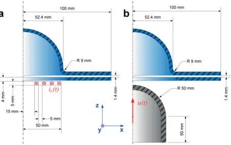
Our analysis is concerned with the introduction of a hemispherical dome (of 50 mm radius) into an initially flat 1.4 mm thick steel sheet (see Fig.1). Two different high speed loading scenarios are considered to achieve this: (1) electro-magnetic loading, and (2) mechanical impact loading. The goal is to compare these two techniques and to come up with an explanation of the well-known failure retardation in forming processes through electro-magnetic load application.
aCorresponding author:[email protected]
2.1. Electro-magnetically applied load
The magnetic field is created by circulating a pulsed electric current through a coil that is positioned next to a conductor material. Figure 2 shows a serial RLC circuit that provides the required current, with LRLC and
RRLCdenoting the inductance and resistivity of the circuit, respectively. The current of intensity ic(t) circulating through the coil with a resistance Rcoiland an inductance
Lcoil is generated by the sudden discharge of the energy stored in capacitor C. Assuming an equivalent ¯R, ¯L, C circuit, the expression for the current intensity of the underdamped response circuit [1] reads
ic(t)=
V0 ω¯L exp
− ¯R
2 ¯Lt
sin (ωt ), ω=
1 ¯LC −
¯R 2 ¯L
2
(1) withωdenoting the natural frequency.
Figure 1. Schematic view of the EM (a) and mechanical (b)
problems.
Figure 2. Simplified RLC circuit used in the electro-magnetic
loading processes. M represents the mutual inductance.
calculated based Eq. (1) with an initial voltage of V0= 11 kV, a capacitance of C=900µF and an inductance of
L =1µH. The capacitor energy is released rapidly, generating a damped current intensity that is attenuated within about 0.3 ms. The entire forming process will also be completed within this duration.
2.2. Mechanically applied load
In the mechanical process, the sheet is loaded through a hemispherical punch. The duration of a conventional mechanical sheet metal forming process is of the order of seconds, while the typical duration of the electro-magnetic process is about four orders of magnitude shorter. In our comparative study, we consider two mechanical loading scenarios: a slow case that is complete within 1s, and a fast case that completes the forming within 0.3 ms. Moreover, to ensure the direct comparability, the punch velocity history in the fast process is chosen such that it matched the velocity of the dome apex in the electro-magnetic process.
3. Thermo-mechanical constitutive
model
The mechanical constitutive response of the material presented here is based on the work by Mohr et al. [3], which subsequently was modified by Roth and Mohr [4] to take into account strain rate and thermal softening effects.
The model assumes the additive decomposition the strain tensorεas:
ε=εe+εp
(2) with the elastic and plastic parts εe andεp. The elastic strain and Cauchy stress tensors are related through Hooke’s law as follows:
σ =C :ε−εp (3)
where C is the positive-definite fourth-order symmetric tensor that contains the elastic modulus E and the Poisson’s ratioν,
C= νE
(1+ν) (1−2ν)I⊗I+
E
(1+ν)I (4) being I and I the identity second-order and fourth-order tensors, respectively.
The Hill 1948 orthotropic yield function [5] is adopted: φ(σ,α)=σ¯φ(σ)−Y (α,α˙)=0 (5) where Y is a deformation resistance,αis a set of internal hardening variables, and ˙α=dα/dt their time derivative.
¯
σφ is the yield function equivalent stress that can be expressed conveniently with a linear transformation of the stress tensor as follows [6]:
¯ σφ(σ)=
√
σ : P :σ (6)
with the positive-definite fourth-order symmetric tensor,
P=
1 P12 −(1+P12) 0 0 0
P22 −(P12+P22) 0 0 0 1+2P12+P22 0 0 0
P330 0
sym 3 0
3
. (7)
The three independent components P12, P22 and P33 can be expressed as a function of the uniaxial tension yield stresses in three directions with respect to the rolling direction, typically at 0, 45 and 90 degrees and the equi-biaxial tension yield stress [3]. The yield function defines a von Mises yield surface in the case of isotropic yielding being P12=−0.5, P22=1.0 and P33 =3.0. A non-associated flow potential of the form,
¯
σψ(σ)=√σ : G :σ (8) has been chosen to represent the flow rule ˙εp=
˙
The set of internal variables are the equivalent plastic strain, the equivalent plastic strain rate and the temperature; their evolution equations read:
˙¯ εp=λ˙
¯ σψ
¯ σφ,ε¨¯p=
d ˙¯εp
dt = d dt ˙ λσ¯ψ ¯ σφ
,T˙ =λ˙χ
˙¯ εp
ρCp ¯ σψ
(9) where ρ is the mass density andCp is the specific heat. Typically, the temperature increase is assumed to be only due to adiabatic effects and the Taylor-Quinney coefficient χ is assumed to be constant and equal to 0.9. In an isothermal situation such a coefficient would be null. A smooth transition between isothermal and adiabatic conditions is proposed as [4]:
χε˙¯p
=χ0
˙¯ εp−ε˙0
2
3˙εa−2˙¯εp−ε˙0
(˙εa−ε˙0)3 (10) being ˙ε0and ˙εathe limit strain rates for the isothermal and adiabatic domains, respectively.
Isotropic hardening is assumed accounting for strain hardening, strain rate hardening and the thermal softening has been considered independent [7–9]. Therefore, the constitutive response can be conveniently expressed in three separate terms that multiply each other as [4]:
Yε¯p,ε˙¯p,T
=Yεε¯p
Y˙εε˙¯p
YT(T ). (11) The strain hardening is defined as a weighted linear combination of a Swift and Voce laws. It reads:
Yε=αAε0+ε¯p n
+(1−α){σ0+Q1
1−exp−C1ε¯p
(12) where A,ε0, n,σ0, Q1, C1are material constants andαis the weighting coefficient. The strain rate hardening and the thermal softening have the same form as those defined by Johnson and Cook [9],
Yε˙ =1+C ln ˙¯ εp ˙ ε0
,YT =1−
T −Tr
Tm−Tr m
(13) where C and m are material constants, Tr and Tm are the reference and melting temperatures respectively.
The Hosford-Coulomb failure criterion is a stress state dependent failure criterion. The stress state is characterized by the stress triaxialityηand the Lode angle parameter ¯θ. The expression of the equivalent plastic strain to failure is composed of three independent terms. The first term represents the stress-state-dependent failure criterion, while the second and the third are the expressions that introduce the strain rate and temperature effects defined as in [10]. The equivalent plastic strain to failure of the failure criterion is:
¯ εf
p =ε¯ f
η,θ¯
η,θ¯ε¯f ˙ ε ˙¯ εp ¯ εf
T(T ). (14) The independent terms are defined as follows:
¯ εf
η,θ¯ =b (1+c)
1 n
F1a+F2a+F3a
2
1 a
+c (2η+ f1 + f3) −1
n
(15)
F1= f1− f2, F2= f2− f3, F3= f1− f3
f1= 2 3cos
π 6
1−θ¯, f2= 2 3cos
π 6
3+θ¯ (16)
f3 =− 2 3cos
π 6
1+θ¯
¯ εf
˙
ε =1+D4ln ˙¯ εp ˙ ε0
, ¯εTf =1+D5
T −Tr
Tm−Tr (17) where a, b, c, D4 and D5 are material constants. The damage indicator evolution law (failure for D=1) is defined as
˙
D= 1
¯ εf
p
η,θ,¯ ε˙¯p,T
ε˙¯p. (18)
It should be noted that since the model is uncoupled, i.e. no softening due to damage evolution; the damage indicator is not an internal variable of the plasticity model. The time discretized equations were integrated in an elastic predictor-plastic corrector-type set of equations and the return to the yield surface was executed with a cutting plane algorithm. The calibration procedure for the DP590 steel can be found in [4] (see Table1).
4. Numerical set-up
Due to its symmetry conditions only one fourth of the geometry was modeled. The discretization was performed using eight-node reduced-integration solid elements with stiffness-based hourglass control. The die and the punch were modelled as non-conductive rigid bodies. The die was fixed in space, while a displacement u(t) was prescribed to the punch. Six elements over the thickness were used for the work piece, whereas for the die and punch, since they were modelled as rigid bodies, only one element was used through the thickness. The in-plane element size of the plate and dies was 1 mm. The end of the plate was considered to be free of constrains. The only constraint comes from the blanket holder that prevents any specimen motion in z-direction (see Table1).
Table 1. Material constants for the DP590 steel.
ρkg
m3
Cp
J kg◦C
E (GPa) ν χ0 ε˙a
s−1 0
S m
7850.0 420.0 210.0 0.3 0.9 1.379 1.5×10⁶ P12 P22 P33 G12 G22 G33 −0.5000 1.0000 3.0000 −0.4946 0.9318 2.4653
A (MPa) ε0 n σ0(MPa) Q1(MPa) C1 α 1031.00 0.00128 0.199 350.00 324.25 25.92 0.64 C ε˙0
s−1 m T0(◦C) T
r(◦C) Tm(◦C)
0.0136 0.001164 0.921 25.0 25.0 1400.6
a b c n D4 D5
1.970 0.820 0.000 0.199 0.025 0.000
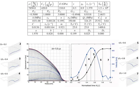
Figure 3. Evolution of the cross-section upper surface depicted in blue in the lateral pictures (left). Displacement and velocity vs.
normalized time of the point located on the center of the plate (right).
5. Results and discussion
Firstly, we analyze the EM forming process and the characteristic steps leading to the final sheet shape. The right hand side plot in Fig. 3 shows the displacement (black) and velocity (blue) histories of the point located in the center of the upper surface of the sheet. The time has been normalized by the total duration of the simulations (tf). The plot is marked with seven solid points that correspond to t/tf =[0.0,0.2,0.4,0.5,0.6,0.8,1.0]. For each of these positions, a snapshot of the deformed geometry was taken (see left and right of Fig. 3). To enhance the visualization of the progressive deformation of the sheet, a cross-section cut along one of the specimen symmetry planes is illustrated in blue over a grid formed by 5×5 mm squares. Additionally, on the left hand side of Fig.3the evolution with time of such cross-section upper line is plotted every 5µs time intervals. The red curves correspond to the initial and final states, t/tf =[0.0,1.0], whereas the blue curves correspond to the intermediate steps, t/tf =[0.2,0.4,0.5,0.6,0.8].
In the initial stage of the plate forming, i.e. from steps one to two, the Lorentz forces generated on the sheet metal plate were concentrated in the area of influence of the coils. As a result, there was a lack of magnetic pressure on the center of the specimen. Its effect on the deformed shape vanished quickly after about 10µs (beyond point two in Fig.3).
From there onwards, the velocity was then transferred from the part driven by Lorentz forces towards the center
of the plate. Moreover, the inertia of the workpiece appeared to be driving the deformation process beyond point four where the velocity was about to reach its maximum (see Fig.3(right)). In the next stage, from point four to five, the displacement of the area close to the center kept displacing at the same pace as it did it the stage before. Conversely, there was a significant loss of velocity that indicated the commencing of the progressive slow-down of the plate (see Fig.3(right)). During the subsequent stage, from step five to six, it suffered a dramatic drop on velocity completing the slow-down process and attaining virtually its maximum displacement. In the last simulated stage, between points six and seven, there were nearly null forces that could affect the deformation of the workpiece. Hence, the center point practically maintained its displacement, while the velocity oscillated around zero.
Figure 4. Evolution with time of the slow (a), EM (b) and fast (c) cases.
Figure 5. Evolution of the thickness with time of the slow (a),
EM (b) and fast (c) cases.
formed made the thinning to be localized within a narrow plastic zone. Therefore, the workpiece necked rapidly in the center area causing its fracture before it reached the pre-established maximum displacement. The progressive thinning and necking on the center area can be seen in Fig.5(a).
The fast case resembles an impact problem, where the punch acts like a guided projectile and the sheet as the target. The only difference here is that the projectile has a prescribed motion in contrast with a typical impact problem. In Fig. 4(c) we observe that even though the principle applied to move the plate was the same as that in the slow case, the plate did not deform in the same way. The center of the workpiece “saw” the contact but the rest of it still did not noticed the impact yet. Figure5(c) depicts perhaps more clearly such phenomenon. There was a stress wave that travelled from the first point where the punch impacted, the center, towards the end of the plate. This relieved such part from strains. There was a moment when the plate did not move by the effect of the punch but by the effect of the inertia. Recall that a similar effect occurred in the in the EM case. The inertia then dragged the central part of the plate, which was not in contact with the punch anymore, necking severely the zone that was highly strained shortly before.
Figure 6. Damage contours of the numerical simulations carried
out for the slow (a), EM (b) and fast (c) cases.
accumulation in the fast case central zone can be clearly seen. In fact, the plastic strain accumulation, as explained before, occurs away from the specimen center. In any case, both slow and fast cases presented a severe thinning and subsequent necking as can be seen in Fig. 5. Conversely to these cases, the more uniform force distribution of the EM case, allowed the plate to thin relatively uniformly and without necking, revealing EM loaded process as the less harmful for the material in terms of fracture. The manner in which the load was applied in this case allowed the strains to distribute more uniformly over the plate and extend the load-applying area not solely to the center, but to far more distance than the mechanically-driven forces allowed. On top of that, the load-applying period was small enough to benefit from strain rate and thermal softening effects which also increase the material’s ductility. Indeed, Fig.6shows how the damage accumulation in the plate is far from the levels of the mechanically loaded cases.
6. Conclusions
This paper presents a computational model predicting the high strain rate failure of electro-magnetically loaded structures. In addition to the electro-magnetic and mechanical solvers, it makes use of a newly-developed rate- and temperature dependent user material subroutine. In particular, the Hill yield surface with a non-associated flow rule was used in conjunction with a Johnson-Cook type of isotropic rate-dependent hardening law. The stress-state, strain-rate and temperature dependent Hosford-Coulomb fracture initiation model was used to evaluate the damage accumulation on the deformation processes.
In a first application, the modeling approach was used to analyze the apparent ductility increase in electromag-netic forming through comparison with simulations with conventional mechanical loading. The analysis showed that the load application in the mechanical cases caused pronounced strain localization within the deforming sheet, whereas significantly more uniform strain distributions are observed for electromagnetic loading. The delayed failure in electromagnetic forming is thus mainly attributed to the increased strain field uniformity, whereas the increase in ductility due to strain rate and temperature effects is seen as secondary.
The first author is grateful for the partial financial support through the French National Research Agency (Grant ANR-11-BS09-0008, LOTERIE).
References
[1] A. Alonso Rodriguez and A. Valli, Eddy Current
Approximation of Maxwell Equations. MS&A, ed.
T.Y. Hou, et al. Vol. 4. (2010): Springer.
[2] V. Psyk, D. Risch, B.L. Kinsey, A.E. Tekkaya, and M. Kleiner, Electromagnetic forming—A review. Journal of Materials Processing Technology, (2011). 211(5): p. 787–829.
[3] D. Mohr, M. Dunand, and K.-H. Kim, Evaluation
of associated and non-associated quadratic plasticity models for advanced high strength steel sheets under multi-axial loading. International Journal of
Plasticity, (2010). 26(7): p. 939–956.
[4] C.C. Roth and D. Mohr, Effect of Strain Rate
on Ductile Fracture Initiation in Advanced High Strength Steel Sheets: Experiments and Mod-eling. International Journal of Plasticity (2014)
(In press).
[5] R. Hill, A theory of the yielding and plastic flow of
anisotropic metals. roceedings of the Royal Society
of London. Series A, Mathematical and Physical Sciences, (1948). 193(1033): p. 281–297.
[6] M.A. Crisfield, Non-linear Finite Element Analysis
of Solids and Structures, Volume 2: Advanced Topics.
(1997), London: John Wiley & Sons.
[7] T. Børvik, Hopperstad, O.S., Berstad, T., Langseth, M., A computational model of viscoplasticity and
ductile damage for impact and penetration. European
Journal of Mechanics – A/Solids, (2001). 20: p. 685–712.
[8] S. Chocron, B. Erice, and C.E. Anderson, A new
plasticity and failure model for ballistic application.
International Journal of Impact Engineering, (2011). 38(8-9): p. 755–764.
[9] G.R. Johnson and W.H. Cook. A Constitutive Model
and Data for Metals Subjected to Large Strains, High Strain Rates and High Temperatures. in 7th International Symposium on Ballistics. (1983). The
Hague.
[10] G.R. Johnson and W.H. Cook, Fracture
character-istics of three metals subjected to various strains, strain rates, temperatures and pressures. Engineering
Fracture Mechanics, (1985). 21: p. 31–48.
[11] P. L’Eplanettenier and I. C¸ aldichoury, EM Theory
Manual, Livermore Software Technology Corpora-tion (LSTC). (2012). 40.
[12] LSTC, LS-DYNA KEYWORD USER’S MANUAL
Version 971 R7.0. (2013), Livermore, California: