Visualization for Molecular Dynamics Simulation of Gas and Metal Surface Interaction

(1)

Visualization for Molecular Dynamics Simulation of Gas

and Metal Surface Interaction

D. Puzyrkov1,a, S. Polyakov1,b, and V. Podryga1,c

1_{Keldysh Institute of Applied Mathematics (Russian Academy of Sciences), Miusskaya sq., 4, Moscow,}

125047, Russia

Abstract.The development of methods, algorithms and applications for visualization of molecular dynamics simulation outputs is discussed. The visual analysis of the results of such calculations is a complex and actual problem especially in case of the large scale simulations. To solve this challenging task it is necessary to decide on: 1) what data parameters to render, 2) what type of visualization to choose, 3) what development tools to use. In the present work an attempt to answer these questions was made. For visual-ization it was offered to draw particles in the corresponding 3D coordinates and also their velocity vectors, trajectories and volume density in the form of isosurfaces or fog. We tested the way of post-processing and visualization based on the Python language with use of additional libraries. Also parallel software was developed that allows processing large volumes of data in the 3D regions of the examined system. This software gives the opportunity to achieve desired results that are obtained in parallel with the calculations, and at the end to collect discrete received frames into a video file. The software package “Enthought Mayavi2” was used as the tool for visualization. This visualization applica-tion gave us the opportunity to study the interacapplica-tion of a gas with a metal surface and to closely observe the adsorption effect.

1 Introduction

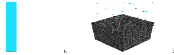
The current stage of the computer technologies development and their computational potential makes it possible the calculation of the properties of complex systems at the molecular and even atomic levels. The mathematical models which describe such processes with the methods of molecular dy-namics (MD) [1] can contain a huge amount of particles, up to several billion, and each particle can have dozens of properties. Such data volumes can amount to terabytes and they make it difficult to study the involved processes properly. It brings us over to the problem of calculation result repre-sentation in a convenient form for further analysis. As we know, MD calculations result in a set of investigated system states, which describes the system evolution over time. For large scale systems the drawing of all the particles is not informative (fig. 1a). In this case it is required to draw not all area of modeling but only the data region of interest (fig. 1b).

(2)

In this work we examine the ability to use the interpreted programming language such as Python [3] for the calculation results analysis and their representation for 3D visualization. Besides the posi-tions of the particles, this visualization should reﬂect diﬀerent parameters, e.g., the temperature, the distribution of the pressure, the particle trajectories. All of that makes necessary the preprocessing of large data amounts. As a test gas-metal system we consider a microsystem [2] consisting of 8552352 particles, where the nitrogen was used as the gas part of the system and the nickel as the metal one.

a b

Figure 1. Nitrogen-Nickel microsystem in the beginning of simulation: entire system in one image (a) and a close up region 10×10×30 nm3_(b)

2 Technologies overview

There are several software packages for atomistic data visualization. For example: PAVMD, VMD, PyMOL, RasMol. A lot of packages for MD calculations (LAMMPS, GROMACS) have their own visualizers. But for using them in any non-standard case (e.g., to visualize a dataset of non-standard format) it is necessary to script them, or convert the data to a well-known format, which is not always possible. In this study we made an attempt to do fast and easy visualization and analysis and to oﬀer the following tools and technologies.

Python [3] is a widely used general-purpose high-level programming language. Its design philoso-phy emphasizes code readability, and its syntax allows programmers to express concepts in fewer lines of code than it would be possible in languages such as C++or Java. The syntax of the Python kernel is very simple and short, at the same time a standard library gives a large volume of useful functions and convenient data structures. Python supports multiple programming paradigms, including object-oriented, imperative and functional programming or procedural styles. It features a dynamic type system and automatic memory management, full introspection, exceptions and multiprocessing. The developers community creates a lot of computer science libraries, that makes Python one of the most commonly used languages for big data analysis and scientiﬁc calculations.

NumPy [5], the open-source package for the Python language, is a free but strong alternative to the proprietary packages for calculations with matrices and vectors (such as MATLAB). Plenty of algorithms for data analysis are implemented at low level, a high quality documentation and detailed examples are provided. All of these advantages make NumPy an ideal choice for the acceleration of scientiﬁc applications in Python language. NumPy oﬀers rich functionality which includes mul-tidimensional arrays, import and export methods, mathematical functions, Fourier transform, linear algebra, etc.

(3)

Table 1.NumPy and Numba+Numpy performance comparison

N NumPy Numba+NumPy rel. performance gain

1000000 0.19ms 0.07ms 2.77

10000000 1.62ms 0.74ms 2.19

100000000 16.06 7,4ms 2.17

from numba i m p o r t j i t

@ j i t ( n o g i l=True , n o p y t h o n=T r u e )

d e f numpy_numba_func ( vx , vy , vz , m u l t i p l i e r₌100 , d i v i d e r₌3 . 0 ) : r e t u r n m u l t i p l i e r∗( ( vx∗vx ) + ( vy∗vy ) + ( vz∗vz ) ) / d i v i d e r

d e f numpy_func ( vx , vy , vz , m u l t i p l i e r=100 , d i v i d e r=3 . 0 ) : r e t u r n m u l t i p l i e r∗( ( vx∗vx ) + ( vy∗vy ) + ( vz∗vz ) ) / d i v i d e r

The productivity increased about 2 times (see table 1). This result was achieved by applying just one decorator and without any other tricks. Of course, Cython [8] (optimizing static compiler for both Python programming language and the extended Cython programming language) will give more performance in this case, but then you should write not pure-python code, and probably think about its optimization.

ParallelPython (PP) [4] has a mechanism for parallelization of a Python code on the SMP systems and scientiﬁc clusters. It is a client-server software, based on the use of “multiprocessing” Python module, and it needs installation on the computational nodes. PP provides a simple application pro-gram interface for the execution of the tasks and getting the results when they are ﬁnished.

Mayavi2 [7] is an instrument for scientific data visualization. It uses Python for general scripting. Mayavi2 allows to deal with large volumes of data in memory, not screening, and then to render an image and save it to file, or show an interactive window. For the individual use of this package it is necessary to develop your own scripts for loading, processing, animating data and for camera control. For the graphics rendering Mayavi2 uses the powerful technology Visualization Toolkit (VTK), which is a data visualization library with open-source code, and it is widely used in the scientific community. Originally, Mayavi2 was developed as a visualization tool for computational hydrodynamics. After the benefit from its usage in other applications became intelligible, it was converted into a general scientific tool for data visualization.

3 Realization details

As an example of dataset, in this work we used the results of the calculations described in [2]. The equilibrium state of the nitrogen-nickel microsystem was calculated using the MD approach. The data obtained in the end of the simulation represents the microsystem states through time. It is a set of binary ﬁles that contains atomistic data, such as particles global indexes, coordinates, velocities, forces, and other properties.

For importing and analysing such structures, we have developed the “mmdlab” package. It pro-vides modules for data reading, processing and common visualization routines.

3.1 mmdlab.datareader module

(4)

to create special storage containers, according to the user-deﬁned description of the particles stored. This method can operate in two diﬀerent ways: fast reading process and operated reading process.

The fast reading process works on the dataset which ﬁts in RAM. It is based on simultaneous loading of all particles and their properties in memory. A vectorized procedure for particle separation into storage containers is performed after the data was loaded and parsed. This process is fast because it makes minimum operations over a single particle in the sequential reading procedure.

The operated reading process takes more time because it sequentially applies a user-defined filter on every particle in the data (for example cutting offthe particles which are out of the specified region or only particles with certain index property). Naturally, the speed of such a filter directly depends on its complexity, however, its advantage is that it doesn’t load into RAM all the data and eventually it gives the storage container with particles which passed the filter.

Every data reading procedure returns the objects of “ParticleContainer” class, that contains proper-ties of the particles assigned to this container by the ﬁlter procedure. After construction, this container automatically calculates temperature and the absolute velocities of every particle assigned to it. This object also contains a user-deﬁned information, for example the atom diameter and its mass.

The Numba+NumPy code for calculation temperatures and velocities looks as simple and clear as a MATLAB code:

from numba i m p o r t j i t i m p o r t numpy

@ j i t

d e f a b s o l u t e _ v e l o c i t y ( vx , vy , vz , m u l t i p l i e r=1 , kb=1 . 3 8 0 6 5 ) :

r e t u r n numpy . s q r t ( ( ( vx_∗vx ) ₊ ( vy_∗vy ) ₊ ( vz_∗vz ) ) )_∗m u l t i p l i e r ; @ j i t

d e f a b s o l u t e _ t e m p ( vx , vy , vz , m, m u l t i p l i e r=100 , kb=1 . 3 8 0 6 5 ) :

r e t u r n m u l t i p l i e r∗m∗( ( vx∗vx ) + ( vy∗vy ) + ( vz∗vz ) ) / ( 3 . 0∗kb )

3.2 mmdlab.dataprocessor module

In the “mmdlab” module we implemented some special methods for atomistic data processing. For example, it has a procedure for post-processing the data filtration by a user-defined filter, a filter for cutting offthe particles not in the specified spatial region and a routine for merging two different containers in a new “ParticleContainer” object, with additional information about the position of every particle from the first container in the second. The last routine is used in the method asking for particle movement interpolation. Let’s consider this feature closely in an application dealing with the particle movement animation task in a user-defined spatial region.

Since the particles can either move into the domain and move out of it, we do not know which of the particles can be in the domain at the next time step. So, ﬁrst of all it is necessary to determine the particles we want to observe. There are two ways to do that:

• pre-process the whole dataset and obtain the particle indexes appearing at least once in a given domain;

• obtain indexes of the particles which were in the given domain at two consecutive time steps and dis-card all the particles that appear in the ﬁrst dataset and do not appear in the second (and vice versa).

It is not possible to use the velocity vector of the particle for the determination of its location in the future steps because the time diﬀerence between system states can be quite large and collisions appear (aﬀecting the velocity).

(5)

array of global indices; 4) import the next dataset, repeat steps 2 & 3; 5) unite two received arrays; 6) remove duplicates; 7) repeat steps 4-6 for every dataset representing system states at diﬀerent times; 8) import ﬁrst and second datasets; 9) merge containers; 10) draw particles movement; 11) repeat steps 8–10 for all dataset pairs (1,2), (2,3), (3,4), . . . , (n−1,n).

Usage of the “mmdlab” package and NumPy+PP for this task is quite simple:

i m p o r t pp

i m p o r t numpy a s np

from mmdlab i m p o r t d a t a r e a d e r , d a t a p r o c e s s o r , u t i l s s e r v = pp . S e r v e r ( n c p u s = 4 )

i n d e x e s = np . a r r a y ( [ ] ) d e f g e t _ i n d e x e s ( f , r e g i o n ) :

c = mmdlab . d a t a r e a d e r . f a s t _ r e a d ( f )

r e t u r n mmdlab . d a t a p r o c e s s o r . r e g i o n _ f i l t e r ( c , r e g i o n ) . i n d e x e s r e g i o n = [ 0 , 1 0 , 0 , 1 0 , 0 , 3 0 ]

p p _ i m p o r t s = (" mmdlab "," mmdlab . d a t a r e a d e r "," mmdlab . d a t a p r o c e s s o r "," mmdlab . u t i l s ") j o b s = [ s e r v . s u b m i t ( g e t _ i n d e x e s , ( f , r e g i o n ) , ( ) , p p _ i m p o r t s ) f o r f i n d a t a f i l e s ] ; f o r j o b i n j o b s :

i n d e x e s = np . u n i q u e ( np . a p p e n d ( i n d e x e s , j o b ( ) ) )

As a result we receive an array, containing all the particle indexes which appear in the specified region at least once. Then it is necessary to import every system state consecutively, filter them for particles the indexes of which are in the obtained array and merge two sequentially read containers in one containing the particle positions in the first and second states.

d e f g e t _ c o n t a i n e r ( f1 , f2 , i n d e x e s ) :

c1 = mmdlab . d a t a p r o c e s s o r . i n d e x _ f i l t e r ( mmdlab . d a t a r e a d e r . f a s t _ r e a d ( f 1 ) , i n d e x e s ) c2 = mmdlab . d a t a p r o c e s s o r . i n d e x _ f i l t e r ( mmdlab . d a t a r e a d e r . f a s t _ r e a d ( f 2 ) , i n d e x e s ) r e t u r n mmdlab . d a t a p r o c e s s o r . merge ( c1 , c2 )

j o b s=[ ]

f o r f i n u t i l s . p a i r s ( d a t a f i l e s ) :

j o b s . a p p e n d ( s e r v . s u b m i t ( g e t _ c o n t a i n e r , ( f [ 0 ] , f [ 1 ] , i n d e x e s ) , ( ) , p p _ i m p o r t s ) ) f o r j o b i n j o b s :

c = j o b ( )

p r i n t c . x [ 0 ] # w i l l p r i n t x c o o r d i n a t e s o f p a r t i c l e s i n f i r s t d a t a s e t

p r i n t c . x [ 1 ] # w i l l p r i n t x c o o r d i n a t e s o f p a r t i c l e s i n s e c o n d d a t a s e t

As for the second option, we define the following algorithm: 1) load the first dataset; 2) apply a cut-off filter to the containers (or use operated reading method for cut-offparticles); 3) repeat steps 1 and 2 for the second dataset; 4) draw particles movement; 5) repeat steps 1–4 for each dataset pair (1,2), (2,3), (3,4), . . . , (n−1,n).

The steps 1 and 2 of the algorithm can be performed with this simple function:

d e f g e t _ c o n t a i n e r v 2 ( f1 , f 2 ) :

c1 = mmdlab . d a t a p r o c e s s o r . r e g i o n _ f i l t e r ( mmdlab . d a t a r e a d e r . f a s t _ r e a d ( f 1 ) , r e g i o n ) c2 ₌ mmdlab . d a t a p r o c e s s o r . r e g i o n _ f i l t e r ( mmdlab . d a t a r e a d e r . f a s t _ r e a d ( f 2 ) , r e g i o n ) r e t u r n mmdlab . d a t a p r o c e s s o r . merge ( c1 , c2 , np . i n t e r s e c t 1 d ( c1 . i n d e x e s , c2 . i n d e x e s ) )

Both algorithms can be parallelized with respect to the data due to the independence of the data at the points [i,i+1] and [i+1,i+2]. ParallelPython does this task perfectly.

(6)

4 Results

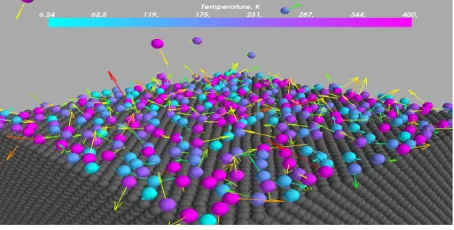
Using the developed “mmdlab” module the visualization and the analysis of the adsorption process which is taking place on the metal-gas border were done (Fig. 2).

Figure 2.Adsorption of nitrogen on the nickel surface. Vectors represent particle velocities direction (in scale), the color represents nitrogen particles temperature.

5 Conclusion

In this work the analysis of the possibility of using the Python language for large scale data processing and visualisation was provided. The accelerators for Python such as NumPy and Numba were studied and put into practice. These packages allow to achieve computation performance comparable with the compiled languages. Also, the developed “mmdlab” module made it possible to visualize and examine in details microsystems with two interacting components. We can see the potential opportunity to use the interpreted programming language Python for processing and visualization problems of molecular dynamics calculations.

This work was supported by the Russian Foundation for Basic Researches (projects No. 13-01-12073-oﬁm, 15-07-06082-a).

References

[1] D.C. Rapaport,The Art of Molecular Dynamics Simulation(Second Edition, Cambridge Univer-sity Press, Cambridge, 2004) 565 p.

[2] V.O. Podryga, S.V. Polyakov, D.V. Puzyrkov, Journal Vychislitel’nye Metody i Program-mirovanie.16, 123–138 (2015) [in Russian]

[3] Oﬃcial site Python, https://www.python.org/

[4] Oﬃcial site ParallelPython, http://www.parallelpython.com/ [5] Oﬃcial site NumPy, http://www.numpy.org/

[6] Oﬃcial site Numba, http://numba.pydata.org/